Diagnostics of stellar flares from X-ray observations: from the decay to the rise phase

Abstract

Context. The diagnostics of stellar flaring coronal loops have been so far largely based on the analysis of the decay phase.

Aims. We derive new diagnostics from the analysis of the rise and peak phase of stellar flares.

Methods. We release the assumption of full equilibrium of the flaring loop at the flare peak, according to the frequently observed delay between the temperature and the density maximum. From scaling laws and hydrodynamic simulations we derive diagnostic formulas as a function of observable quantities and times.

Results. We obtain a diagnostic toolset related to the rise phase, including the loop length, density and aspect ratio. We discuss the limitations of this approach and find that the assumption of loop equilibrium in the analysis of the decay leads to a moderate overestimate of the loop length. A few relevant applications to previously analyzed stellar flares are shown.

Conclusions. The analysis of the flare rise and peak phase complements and completes the analysis of the decay phase.

1 Introduction

Solar and stellar coronal flares are impulsive events well detected in the soft X-ray band. They are typically explained as due to the sudden increase of temperature and emission measure of the plasma confined in single or groups of magnetic tubes (loops), caused by strong heat pulses.

The flare light curves in the soft X-rays are typically characterized by a fast rise phase followed by a slower decay (e.g. Haisch et al. 1983). In the decay phase, the plasma cooling is due to radiation emission and to thermal conduction to the chromosphere. Since the cooling times for a confined plasma depend on the characteristics of the confining structure, and in particular on its length, the analysis of the decay phase has been extensively used to diagnose the flaring loops, and in particular their size (see Reale 2002 for an extensive review). This is important not only because stellar flaring regions are unresolved, but also because, more in general, this is one of the few tools to obtain detailed information on the geometry of the stellar coronae (e.g. Favata et al. 2000a), and of any other phenomena involving plasma confined in magnetic structures.

To summarize, Serio et al. (1991) derived a thermodynamic time scale for the pure cooling of flaring plasma confined in single coronal loops:

$$\tau_{s}=3.7\times 10^{-4}\frac{L}{\sqrt{T_{0}}}=120\frac{L_{9}}{\sqrt{T_{0,7}}}$$ (1)

where $L$ ($L_{9}$) the loop half-length (in units of $10^{9}$ cm), $T_{0}$ ($T_{0,7}$) the loop maximum temperature (in units of $10^{7}$ K). In principle, the loop length can be derived simply by inverting Eq.(1). Jakimiec et al. (1992) and Sylwester et al. (1993) analyzed extensively the decay of solar coronal flares and pointed out that significant heating can be released even during the late phases of a flare. This can be diagnosed through the analysis of the path of the decay in a density-temperature diagram: sustained heating slows down the plasma cooling but much less the density decrease. If this effect is not properly taken into account, the loop length can be significantly overestimated. Reale et al. (1997) use the scale time Eq.(1) to derive a formula for loop length, corrected to include the effect of significant heating in the decay (see the Appendix for a review). This approach has been extensively applied to analyze observed stellar flares (see Reale 2003 for a review), with the exception of flares where the residual heating completely drives the flare decay over the plasma cooling. These flares are more appropriately described with models of two-ribbon flares (Kopp & Poletto 1984).

Eq.(1) and all the subsequent derivations lie on the assumption that the flare decay starts when the loop is at hydrostatic and energy equilibrium. Extensive modeling of solar and stellar flares has shown that the heat pulses that trigger the flare are impulsive, i.e. their duration is small with respect to the overall flare duration. One then wonders whether the flaring loop has had enough time to reach equilibrium before the heat pulse is switched off or not, and, if not, whether this might be important for the analysis of the decay. Jakimiec et al. (1992) showed that temperature and density begin to decrease simultaneously if the heating lasts long enough to reach equilibrium. In many flares, it is instead observed that the temperature peaks (and therefore begins to decrease) measurably before the emission measure, both in solar flares (e.g. Sylwester et al. 1993) and in stellar flares (van den Oord et al. 1988, van den Oord et al. 1989, Favata et al. 1999, Favata et al. 2000b, Stelzer et al. 2002). Cargill & Klimchuk (2004) pointed out that in transiently heated loops the cooling is initially dominated by thermal conduction and that the density begins to decay as soon as the radiative and conduction cooling times become equal.

Most attention has been so far dedicated to the decay phase, which is the longest-lasting part of flares and therefore typically offers more opportunities of time-resolved data analysis and of good photon statistics. Little and partial attention has been instead devoted to the initial phase of the flares. Hawley et al. (1995) study the rise phase jointly to the decay phase, including neither the heating in the decay, nor the delay between the temperature and the density peak.

Flare observations from recent missions such as Chandra and XMM-Newton often detect flares in great detail and succeed in resolving the rise phase (e.g. Güdel et al. 2004). On the other hand, in long flares it happens that the observations ends early in the decay phase, inhibiting the related analysis and making any kind of information derivable from the rise phase important (e.g. Giardino et al. 2004).

In this work, we address specifically the rise and peak phase of flares, and investigate what diagnostics can be extracted from its analysis. We will study the flare initial phases as a stand-alone analysis, and compare and cross-check with the analysis of the decay. We will also address possible additional diagnostics, e.g. the density and the loop aspect ratio cross-section radius over length – are flaring loops fat or slim or arcades of loops? – which cannot be constrained just from the decay analysis. In our derivation, we will maintain the assumption that the flare occurs in a single loop. This assumption is more realistic in the rise phase, when the impulsive heating typically involves a dominant loop structure while later residual heating may be released in other similar adjacent loops (e.g. Aschwanden & Alexander 2001). We will instead release the assumption that the flaring loop evolves to a condition of equilibrium, and therefore also address the question of what is the effect of releasing equilibrium conditions on diagnostic formulae, i.e. if the decay starts before the loop reaches equilibrium conditions, and what is the error from assuming equilibrium conditions. We will derive the loop length from the rise phase.

In Section 2, we analise the flare evolution with a general outline, operative definitions, relevant results from modeling. In Section 3, diagnostic tools for the analysis of the flare rise and peak phase are derived. In Section 4, we discuss the results, the limitations of the analysis, the applications, with some specific examples and in Section 5 we draw our conclusions.

2 Flare analysis

2.1 General flare evolution

We consider a flare occurring in a single coronal loop. A flaring coronal loop can be modelled as a magnetic flux tube where the plasma is heated to flare temperatures by a transient heat pulse. The plasma confined in the loop can be described as a compressible fluid which moves and transports energy along the magnetic field lines (e.g. Priest 1984).

We will suppose that: (i) the flare occurs in a semicircular loop with half-length $L$, initially in equilibrium conditions at much lower temperature and density than at flaring conditions; (ii) the flare is triggered by a heat pulse uniformly distributed in the loop; (iii) the heat pulse is a top-hat function in time; (iv) there is no heating in the decay; (v) the flaring loop is much smaller than the pressure scale height at the flare temperature.

The plasma cooling is governed by the thermal conduction to the cool chromosphere and by radiation from optically thin conditions. The evolution of the confined plasma is well-known from observations and from modeling (e.g. Nagai 1980, Peres et al. 1982, Cheng et al. 1983, Nagai & Emslie 1984, Fisher et al. 1985, MacNeice 1986, Betta et al. 2001) and in the following we summarize it into four phases, sketched in Fig. 1, which map on the path drawn in the density-temperature diagram of Fig. 2 (see also Jakimiec et al. 1992).

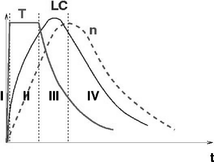
Figure 1: Scheme of the evolution of temperature (T, thick solid line), X-ray emission (LC, thinner solid line) and density (n, dashed line) during a flare triggered in a coronal loop by a heat pulse. The flare evolution is divided into four phases (I, II, III, IV, see text for further details).

Phase I

: from the start of the heat pulse to the temperature peak (heating). The heat pulse is triggered in the loop and the heat is efficiently conducted down to the much cooler and denser chromosphere. The temperature rapidly increases in the whole loop, with a time scale given by the conduction time in a low density plasma (see below).

Phase II

: from the temperature peak to the end of the heat pulse (evaporation). The temperature settles to the maximum value ($T_{0}$). The chromospheric plasma is strongly heated and expands upwards, filling the loop with much denser plasma. The evaporation is explosive at first, with a timescale given by the isothermal sound crossing time:

$$\tau_{sd}=\frac{L}{\sqrt{2k_{B}T_{0}/m}}\approx 25\frac{L_{9}}{\sqrt{T_{0,7}}}$$ (2)

where $k_{B}$ is the Boltzmann constant, $m$ is the average particle mass. After the evaporation front has reached the loop apex, the loop continues to fill more gently. The time scale during this more gradual evaporation is dictated by the time taken by the cooling rate to balance the heat input rate (see Sec. 3).

Phase III

: from the end of the heat pulse to the density peak (conductive cooling). When the heat pulse stops, the plasma immediately starts to cool due to the efficient thermal conduction (e.g. Cargill & Klimchuk 2004), with a time scale:

$$\tau_{c}=\frac{3n_{c}k_{B}T_{0}L^{2}}{2/7\kappa T_{0}^{7/2}}=\frac{10.5n_{c}k_{B}L^{2}}{\kappa T_{0}^{5/2}}\approx 50\frac{n_{c,10}L_{9}^{2}}{T_{0,7}^{5/2}}$$ (3)

where $n_{c}$ ($n_{c,10}$) is the particle density ($10^{10}$ cm^-3) at the end of the heat pulse, $\kappa=9\times 10^{-7}$ (c.g.s. units) is the thermal conductivity.

The heat stop time can then be generally traced as the time at which the temperature begins to decrease significantly and monotonically. While the conduction cooling dominates, the plasma evaporation is still going on and the density increasing. The efficiency of radiation cooling increases as well. On the other hand, the efficiency of conduction cooling decreases with the temperature.

Phase IV

: from the density peak afterwards (Radiative cooling). As soon as the radiation cooling time becomes equal to the conduction cooling time (Cargill & Klimchuk 2004), the density reaches its maximum, and the loop depletion starts, slow at first and then progressively increasing. The pressure begins to decrease inside the loop, and is no longer able to sustain the plasma. In this phase, radiation becomes the dominant cooling mechanism, with the following time scale:

$$\tau_{r}=\frac{3k_{B}T_{M}}{n_{M}P(T)}=\frac{3k_{B}T_{M}}{bT_{M}^{\alpha}n_{M}}\approx 9\times 10^{3}\frac{T_{M,7}^{3/2}}{n_{M,10}}$$ (4)

where $T_{M}$ ($T_{M,7}$) is the temperature at the time of the density maximum ($10^{7}$ K), $n_{M}$ ($n_{M,10}$) the maximum density ($10^{10}$ cm^-3), $P(T)$ the plasma emissivity per unit emission measure, expressed as:

$$P(T)=bT^{\alpha}$$

with $b=1.5\times 10^{-19}$ and $\alpha=-1/2$, for consistency with the parameters of the loop scaling laws (Rosner et al. 1978). In this phase, the density and the temperature both decrease monotonically. The presence of significant residual heating could make the decay slower. This can be diagnosed from the analysis of the slope of the decay path in the density-temperature diagram (Sylwester et al. 1993, Reale et al. 1997, see the Appendix).

2.2 Heat pulse duration

The evolution outlined in Sec. 2.1 concerns a flare driven by a transient heat pulse. The analysis of stellar flares based on the decay phase typically assumes that the decay starts from equilibrium conditions, i.e. departing from the the locus of the equilibrium loops with a given length (hereafter QSS line, Jakimiec et al. 1992) in Fig. 2. The link between this assumption and the flare evolution outlined above is shown in Fig. 2: if the heat pulse lasts long enough, phase II extends to the right, and the flaring loop asymptotically reaches equilibrium conditions, i.e. the horizontal line approaches the QSS line. It is worth noting that, if the decay starts from equilibrium conditions, Phase III is no longer present, and Phase II links directly to Phase IV. Therefore, there is no delay between the beginning of the temperature decay and the beginning of the density decay: the temperature and the density start to decrease simultaneously. Also, the decay will be dominated by radiation cooling, except for its very beginning (Serio et al. 1991).

Figure 2: Scheme of the flare evolution of Fig. 1 in a density-temperature diagram (solid line). The four phases are labelled. The locus of the equilibrium loops is shown (dashed-dotted line), as well as the flare path with an extremely long heat pulse (dashed line). The corresponding decay path (marked with EQ) is the one typically considered by flare analysis based on the decay phase.

The analysis of the rise and peak phase has to include the presence of Phase III, and the delay between the temperature peak and the density peak. This delay is often observed both in solar flares (e.g. Sylwester et al. 1993) and in stellar flares (e.g. van den Oord et al. 1988, 1989, Favata et al. 2000b, Maggio et al. 2000, Stelzer et al. 2002). The presence of this delay is a signature of a relatively short heat pulse, or, in other words, of a decay starting from non-equilibrium conditions.

2.3 Hydrodynamic modeling

We now use hydrodynamic simulations to analyze more in detail the evolution of the rise and peak phase of a flare (Phases I to III). The Palermo-Harvard code solves the time-dependent hydrodynamic equations for the plasma confined in a loop to describe the evolution of the density, temperature and velocity of the plasma along the loop (Peres et al. 1982, Betta et al. 1997).

As a representative example, we consider an initially quiet coronal loop with half-length $L=2\times 10^{9}$ cm and temperature of about 3 MK. A transient heat pulse is injected in it at time t=0. The flare heat pulse lasts for a time $t_{heat}$, is uniformly distributed in the loop, and is as intense (9 erg cm^-3 s^-1) as to bring the loop to a temperature of $\sim 20$ MK.

Figure 3: Evolution of the plasma temperature (top panel), density (middle) and pressure (bottom) at the loop apex, as computed from a hydrodynamic model of a 20 MK flare in a loop with half-length $L=2\times 10^{9}$ cm, and with three different durations of the heat pulse (labelled in the top panel, in units of $\tau_{s}$) and with non-stopping heating. The asymptotic density and pressure values are also shown (dotted horizontal lines). The time of the density maximum is marked (black spots).

Fig. 3 shows the evolution of the plasma temperature, density and pressure at the loop apex for three different durations of the heat pulse (i.e. $t_{heat}=90$ s $\approx 0.5\tau_{s}$, $t_{heat}=170$ s $\approx\tau_{s}$ and $t_{heat}=500$ s $\approx 3\tau_{s}$) and for non-stopping heating. As long as the heat pulse is on, the simulation results overlap; they differ only for the decay phase, when the heating is off. The decay of the simulations with longer-lasting heat pulses begins later. As already mentioned in Sec. 2.1, the temperature begins to decrease as soon as the heat pulse stops. The density and the pressure, instead, both continue to increase and they reach their maximum well later. We note that the shorter the heat pulse, the longer is the delay between the beginning of the temperature decay and the density maximum. For the longest-lasting heat pulse, the density and pressure values are very close to the asymptotic equilibrium values, estimated from loop scaling laws (Rosner et al. 1978). We have checked that the evolution is self-similar for a longer loop $L=10^{10}$ cm at the same temperature, with the evolution times scaling as $\tau_{s}$.

Figure 4: Evolution of the flare of Fig. 3 in the density-temperature diagram. The locus of the equilibrium loops derived from loop scaling laws (QSS curve, dashed line) is also shown.

In the density-temperature diagram (Fig. 4), the flare evolution for the different heat pulse durations is well in agreement with that sketched in Fig. 2. For short-lasting pulses, phase IV starts as soon as the path crosses the QSS curve. For $t_{heat}\approx 3\tau_{s}$, phase II ends and the decay (phase IV) starts both very close to the QSS curve, while phase III is practically absent (Jakimiec et al. 1992).

3 Diagnostics of the rise and peak phase

We now derive simple diagnostic tools for the analysis of the rise and decay phase of a flare, taking advantage of detailed numerical modeling. We first observe that the maximum possible duration of the rise phase is the time taken by the loop to reach equilibrium conditions under the action of a constant (flare) heating. The simulation results in Fig. 3 show that the time taken by the plasma to reach equilibrium conditions is much longer than the sound crossing time (Eq.[2]), which rules the very initial plasma evaporation. This is also clear in Fig. 5, which shows the evolution of the pressure at the loop apex in a linear scale: after $t=50$ s, the rate of pressure enhancement becomes more gentle. As mentioned in Sec. 2.1, in this phase the dynamics become much less important and the interplay between cooling and heating processes becomes dominant. The relevant time scale is therefore that reported in Eq. (1).

After detailed analysis of extensive numerical modeling of decaying flaring loops, we have checked that the decay time from Eq. (1) should be computed with a correction factor:

$$\tau^{\prime}_{s}=\phi\tau_{s}$$ (5)

where $\phi\approx 1.3$ to better fit the decay time measured from numerical models.

Figure 5: Pressure evolution of the flare of Fig. 3 in a linear scale to show that most of the rise phase can be reasonably described with a linear trend (dashed lines).

Hydrodynamic simulations confirm that the time required to reach full equilibrium scales as the loop cooling time ($\tau_{s}$), and, as shown for instance in Fig. 5 (see also Jakimiec et al. 1992), the time to reach flare steady-state equilibrium is:

$$t_{eq}\approx 3\tau_{s}\approx 2.3\tau^{\prime}_{s}$$ (6)

We have verified that Eq.(6) holds for loops of different lengths. Fig. 6 shows the ratio of the time required to reach 97% of the pressure equilibrium value to the time computed from Eq. (6) for simulations of flaring loops with three different loop lengths, and three different heating rates appropriate to reach the temperature of 10, 20 and 30 MK, respectively. The agreement is within 10%.

Figure 6: Time to reach pressure equilibrium obtained from hydrodynamic simulations: the ratio of the time at which the pressure is 97% of the equilibrium value to the time obtained from Eq. (6) vs loop length. The size of the data points is proportional to the heating rate (maximum temperature of 10, 20 and 30 MK).

For $t\geq t_{eq}$, the density asymptotically approaches the equilibrium value:

$$n_{0}=\frac{T_{0}^{2}}{2a^{3}k_{B}L}=1.3\times 10^{6}\leavevmode\nobreak\ \frac{T_{0}^{2}}{L}$$ (7)

where $a=1.4\times 10^{3}$ (c.g.s. units), or

$$n_{0,10}=13\frac{T_{0,7}^{2}}{L_{9}}$$

as obtained from the loop scaling laws (Rosner et al. 1978) and the plasma equation of state.

If the heat pulse stops before the loop reaches equilibrium conditions, the flare maximum density is lower than the value at equilibrium. Fig. 5 shows that, after the initial impulsive evaporation on a time scale given by Eq.(2), the later progressive pressure growth can be approximated with a linear trend. Since the temperature is almost constant in this phase (Fig. 3), we can as well approximate that the density increases linearly for most of the time. We can then estimate the value of the maximum density at the loop apex as:

$$n_{M}\approx n_{0}\frac{t_{M}}{t_{eq}}$$ (8)

where $t_{M}$ is the time at which the density maximum occurs, which can be measured directly from observations. Since it is reasonable to assume that the volume of the flaring region does not change much, at least on the relatively short time scale of the rise phase, the time of the maximum emission measure is a good proxy for $t_{M}$.

Phase III ranges between the time at which the heat pulse ends and the time of the density maximum. Fig. 3 shows that the start time of the temperature decay marks well the end of the heat pulse. In many stellar flares, the temperature evolution is not well resolved, and we may take the time of the temperature maximum as indicative of the end of the heat pulse.

The time of the density maximum is also the time at which the decay path crosses the locus of the equilibrium loops (QSS curve). As reported in Sec. 2.1, Cargill & Klimchuk (2004) remarked that, at this time, the radiative cooling time is exactly equal to the conductive cooling time. By equating the time scales in Eqs. (4) and (3), we can then derive the temperature $T_{M}$ at which the flare maximum density occurs:

$$T_{M}=9\times 10^{-4}(n_{M}L)^{1/2}$$ (9)

or

$$T_{M,7}=0.28(n_{M,10}L_{9})^{1/2}$$

If a value for $L$ is already available to us and we are able to measure $T_{M}$, we can derive $n_{M}$ from Eq.(9), in alternative to Eq.(8).

Since phase III is dominated by conductive cooling, we derive its duration, i.e. the time from the end of the heat pulse to the density maximum, as

$$\Delta t_{0-M}\approx\tau_{c}\ln\psi$$ (10)

where

$$\psi=\frac{T_{0}}{T_{M}}$$

and $\tau_{c}$ (Eq.[3]) is computed for an appropriate value of the density $n_{c}$. A good consistency with numerical simulations is obtained for $n_{c}=(2/3)n_{M}$.

The collection of Eqs. (6) – (10) provides a set of diagnostic tools for the analysis of the rise and peak phase of stellar flares. Eqs. (6) – (8) are related to the rise phase, the others to the peak phase, or, more precisely, phase III as defined in Sec. 2.1. We have checked that the equations provide values consistent with those obtained from accurate numerical modeling within few percent.

By combining Eq.(10) and Eq.(8) we obtain:

$$\frac{\Delta t_{0-M}}{t_{M}}\approx 1.2\ln\psi$$ (11)

which ranges between 0.2 and 0.8 for typical values of $\psi$ (1.2 – 2).

By combining Eqs.(7), (8) and (9), we derive a new expression for the loop half length:

$$L_{9}\approx 3\leavevmode\nobreak\ \psi^{2}T_{0,7}^{1/2}t_{M,3}$$ (12)

where $t_{M,3}$ is $t_{M}$ in units of $10^{3}$ s. For typical values of $\psi$ and $T_{0}$, we obtain $L_{9}\sim 5-25t_{M,3}$ and $L_{9}\sim 10t_{M,3}$ may be taken for rough estimates. Therefore, we expect that flares occurring in loops with length of the order of $10^{10}$ cm show the peak of the emission measure about 1 ks after the beginning.

By including Eqs.(11) into Eq.(12), we derive another alternative expression for the loop half length:

$$L_{9}\approx 2.5\leavevmode\nobreak\ \frac{\psi^{2}}{\ln\psi}T_{0,7}^{1/2}\Delta t_{0-M,3}$$ (13)

where $\Delta t_{0-M,3}$ is $\Delta t_{0-M}$ in units of $10^{3}$ s. For typical values of $\psi$ and $T_{0}$, we obtain $L_{9}\sim 20-100\Delta t_{0-M,3}$ and $L_{9}\sim 50\Delta t_{0-M,3}$ may be taken for rough estimates.

The loop length derived from application of Eqs.(12) and (13) to the model simulations is correct within $10\%$. Eqs.(12) and (13) allow us to estimate the length of the flaring loop from measuring characteristic time intervals of the flare rise phase and related temperatures.

4 Discussion: implications and applications

4.1 Consistency and limitations

The aim of this work is to investigate the diagnostics of the rise and peak phase of coronal flares, to complement the well-established diagnostics of the decay phase (e.g. Reale et al. 1997). Once derived the relevant diagnostic expressions, we first check whether there are effects on the analysis of the decay. In particular, we wonder whether assuming that the decay starts from loop equilibrium conditions – therefore ignoring the details of the “previous history” – leads to significant systematic errors or not. In the decay analysis, one important parameter is the temperature at the start of the decay. At equilibrium conditions, the decay starts at the temperature maximum. In Sec. 2.1, we have pointed out that, in an impulsive flare event, in which the loop does not reach equilibrium conditions, the density begins to decay later than the temperature. The proper decay phase begins at the density peak (i.e. the later time), and one should then use the temperature at the density peak, lower than the maximum temperature. The proper loop decay time then becomes:

$$\tau_{d}=\sqrt{\frac{T_{0}}{T_{M}}}\tau^{\prime}_{s}$$ (14)

If we use the maximum temperature $T_{0}$ to estimate the loop length with expressions derived from Eq. (1) (Reale et al. 1997), instead of $T_{M}$, we then overestimate the loop length. However, since the dependence on the temperature is rather weak in Eq.(1) and the temperatures not very different, we expect not a too large effect on previous results. The error can be easily estimated from the square root of the ratio of the maximum temperature to the temperature at the density maximum. Since this ratio is typically of about 1.2-1.5 (see Sec.4.5), the amount of overestimate is no more than 15-20%. Furthermore, if we know this ratio we can correct for this effect.

Figure 7: Time of the density maximum ($t_{M}$, solid line), delay of the beginning of the density decay from that of the temperature decay ($\Delta t_{0-M}$ , dashed line), and loop decay time ($\tau_{d}$, dotted line) vs the duration of the heat pulse $t_{heat}$. All times are in units of the equilibrium decay time $\tau^{\prime}_{s}$.

Fig. 7 shows how the decay time varies with the duration of the heat pulse. As expected, the decay time is invariably larger than the equilibrium decay time: the shorter the heat pulse, the longer is the decay time, with a maximum of about 1.7 $\tau^{\prime}_{s}$. However, in most of the range, the decay time is larger no more than $20\%$ than the equilibrium decay time, and therefore the loop length overestimated by the same amount.

In all the above analysis we have neglected the effect of the star gravity. This is reasonable both because the gravity have very little influence on the strong initial flare dynamics, and because, at the high temperatures of stellar flares, the pressure scale height:

$$h_{p}\sim 5000\frac{T}{g_{*}/g_{\odot}}=50\frac{T_{7}}{g_{*}/g_{\odot}}$$

is larger than the height of the flaring loops (assuming they stand vertical on the stellar surface). For very long loops, comparable to the stellar radius, the pressure scale height is even longer because the gravity decreases significantly at long distances from the surface, so that the effect of gravity is expected to be even smaller.

Finally, throughout our analysis we have assumed a simple heating function: a top-hat in time, uniform distribution in space. Different heating functions may have some effects on the results (somewhat discussed in Sec. 4.5), but except for very extreme cases, most of them should be smoothed out by the very efficient thermal conduction.

4.2 Loop length from the rise phase

Stellar flare observations do not always cover the whole flare duration; sometimes the rise phase is missing, sometimes most of the decay is not observed. The latter possibility can occur quite frequently, because the decay is the longest part of the flare and, for long flares, the observation may end too early in the decay. One result of the present work is to provide a set of useful formulae for events with missing observed decay. This could be obtained ultimately because most of the rise phase is ruled by the same processes which rule the decay phase, i.e. the energy losses. Eq.(12) yields the loop length, from the time of the maximum density $t_{M}$ (the emission measure can be used as a proxy), the maximum temperature $T_{0}$ and the temperature at the density maximum $T_{M}$.

Alternatively, we may derive the loop length from Eq.(13) even if we miss the flare start but we are able to measure the time interval between the temperature maximum and the density (or emission measure) maximum. If both times are available to us, we may choose the less uncertain one as the more reliable, and we may use both of them to check for consistency and to derive a more accurate length value from a weighted average. We should in fact consider that the determination of the relevant flare times can be affected by significant uncertainties. The time of the density maximum is typically determined within a time bin where the spectral fitting is performed. This time bin can be quite large. Moreover, it is reckoned from the time of the flare start, which can in turn be not well-determined. Analogously, the uncertainty in the interval $\Delta t_{0-M}$ comes from the width of both the time bins including the temperature maximum and the density maximum. The strong dependence on the ratio $\psi=T_{0}/T_{M}$ can also add to further uncertainties.

Eqs.(12) and (13) provide the loop length even if only the rise and peak phase of the flare are observed. These expressions are alternative and independent of the expressions based on the flare decay and therefore of the presence of any significant heating during the decay. They can provide therefore a further check on the loop length estimation, if both loop length values are available. There is a chance to obtain inconsistent results from the two approaches if the flare decay progressively involves other different coronal loops, or else if the heat pulse triggering the flare is not a top-hat function, instead, for instance, slowly rising.

If no time-resolved spectral information is available, e.g. because of low photon statistics, the time of the light curve maximum may be used as a proxy of the time of the emission measure maximum. Since the former occurs a bit earlier than the latter, the loop length estimated from the former will be slightly underestimated.

4.3 Loop Cross-section

A typical output of the analysis of X-ray spectra with moderate resolution, such as those from CCD detectors (e.g. EPIC/XMM-Newton, ACIS/Chandra), is the emission measure associated with a fit thermal component. Time-resolved spectra during the flare can then provide us with the flare maximum emission measure. If we know also the maximum density, we can then derive the loop volume, and, knowing the loop length, also the loop cross-section area and radius. From Eq.(8) and/or Eq.(13) we can evaluate the maximum density at the loop top. Since the emission measure is integrated over most of the loop (the part emitting in the instrument band), For consistency, the volume should be computed using the density averaged of the emitting part of the loop. In realistic conditions of pressure equilibrium, this average density is higher than the density at the loop apex, because the temperature decreases downwards from the loop apex. A reasonable estimate of this average density can be derived from the expressions linking the loop apex temperature to the temperature obtained from spectrum fitting (e.g. Favata et al. 2000b), under the reasonable assumption that the fit temperature is an average loop temperature:

$$T_{M}=\xi\leavevmode\nobreak\ T_{avg}^{\eta}$$ (15)

where the parameters $\xi$ and $\eta$ depend on the observation instrument (e.g. $\xi=0.130$ and 0.233 and $\eta=1.16$ and 1.099 for EPIC/XMM-Newton, and MECS/BeppoSAX, respectively, see also the Appendix, Eq. 21). Then the average density is:

$$n_{avg}=n_{M}\frac{T_{M}}{T_{avg}}$$ (16)

Typically $n_{avg}/n_{M}\sim 1.5-2$. The loop volume $V$, cross-section area $A$ and radius $R$ are then:

$$V\approx\frac{EM}{n_{avg}^{2}}$$ (17)

$$A\approx\frac{V}{2\leavevmode\nobreak\ L}$$ (18)

$$r\approx\sqrt{\frac{A}{\pi}}$$ (19)

The final results of such formulae should be in any way taken with care, because highly indirect and therefore strongly affected by the error propagation.

4.4 Single loop versus multi-loop

It has been pointed out that large and long stellar flares likely involve entire coronal regions including multiple loop structures. How can one reconcile this remark with the single loop approach followed in this work? Of course, since telescopes are not powerful enough to resolve the flaring structures, we cannot give conclusive answers. However, a few arguments can support our single loop approach.

If multiple loop structures are involved in the flare, this frequently occurs in the late phases of a flare. The initial phases of an X-ray flare are instead quite localized and one can reasonably assume the presence of a single dominant loop, at least in the rise phase. This is observed in solar X-ray flares (e.g. Aschwanden & Alexander 2001) and supported by the accurate modeling of a well-observed stellar flare at least in the rise, peak and early decay (Reale et al. 2004). The clear evidence of a delay between the temperature and the density peak in many flares is consistent with a single loop model. Even in the later flare phases, a decay with no significant heating, i.e. with a steep path in the density-temperature diagram as sometimes observed even in very large flares (e.g. Favata et al. 2005) suggests strong plasma cooling confined in single loops. Arcades and two-ribbon flares are instead characterized by strong heating which completely dominates the flare decay (e.g. Kopp & Poletto 1984) and/or by irregular light curves (Aschwanden & Alexander 2001, Reale et al. 2004). Recently, multi-thread models have been used to study solar flare evolution (Warren & Doschek 2005, Warren 2006). In this case, the hydrodynamics of the threads will be described by the results presented here.

4.5 Sample applications

As sample applications of the analysis described above, we have revisited three stellar flares already studied in the literature: a flare on Algol observed with BeppoSAX on 30 August 1997 (Schmitt & Favata 1999, Favata & Schmitt 1999), a flare on AB Doradus observed with BeppoSAX on 29 November 1997 (Maggio et al. 2000) and a flare on Proxima Centauri observed with XMM-Newton on 12 August 2001 (Güdel et al. 2004, Reale et al. 2004). The first flare is quite long ($\sim 1$ day) and shows an eclipse in the late decay phase. The first two flares are also hot (above 100 MK) and quite big, involving an emission measure above $10^{54}$ cm^-3. The last flare is cooler and on a smaller scale, but observed in great detail, thanks to the short distance of Proxima Centauri. It has been modelled accurately with detailed time-dependent hydrodynamic simulations (Reale et al. 2004), obtaining constraints even on the time and space distribution of the heating. These flares have been selected because for all of them the parameters related to the present analysis are all available with the associated uncertainties, and the uncertainties themselves are not excessively large.

Table 1 shows the results obtained from Eqs.(8)–(19) for these three flares. The data in the first ten rows are derived from the original analysis of the references cited in the table. The first four are characteristic times, the light curve decay time ($\tau_{LC}$), the time of the temperature maximum ($t_{0}$), and of the density maximum ($t_{M}$) reckoned since the beginning of the flare, and the delay between the temperature and the density maximum ($\delta t_{0-M}$). There are then the flare maximum temperature ($T_{obs}$) and emission measure ($EM$) as derived from one-temperature fitting, and the ratio of the maximum temperature to the temperature at the density maximum. The loop maximum temperature ($T_{0}$), the half-length ($L$) and the thermodynamic cooling time ($\tau_{s}$) are derived more indirectly according to empirical formulae (e.g. Reale et al. 1997, see the Appendix).

The last ten rows show results obtained with the analysis presented in this work. The first four are densities: the loop equilibrium density ($n_{0}$) pertaining to the derived maximum temperature ($T_{0}$), the actual maximum density ($n_{M}$) derived in two different ways, and the maximum density averaged over the whole loop ($n_{avg}$), derived from the first maximum density. Then there are the loop volume ($V$), cross-section area ($A$), and radius ($r$). Finally, we show other three values of the loop length: the first one is a refinement of the original length derivation, using the temperature at the density maximum ($T_{M}$), instead of the maximum temperature ($T_{0}$). Since $T_{M}\leq T_{0}$, the new length is invariably smaller than the original, but not by large factors, as discussed in Sec.4.2 (within 20%), thus mostly confirming the results of the previous analyses. The other two length values are obtained from the analysis of the rise and peak phase, presented here (Eqs. [12] and [13]).

The first two flares show a significant delay of the time of the density maximum from that of the temperature maximum – an indication that the heat pulse is relatively short as compared to the loop characteristic cooling time. Coherently, the ratio of the maximum temperature to the temperature at the density maximum is relatively large (e.g. Fig.3). The flare on Proxima Centauri shows instead a relatively smaller delay and a coherently smaller temperature ratio. The loop length and the decay time are very large for the first flare ($\sim 10^{12}$ cm and 21 ks, respectively) and much smaller for the other two.

In all flares, the plasma does not reach equilibrium conditions, and the maximum density is well below the equilibrium density. Although different, Eqs.(8) and (9) yield consistent density values – within the (quite large) uncertainties – for all flares, between a few $10^{10}$ cm^-3 and a few $10^{11}$ cm^-3. The loop volume and cross-section parameters are affected by even larger uncertainties; they are derived from the combination of several quantities and suffer from the error propagation. It is nevertheless confirmed the large loop aspect ratio for the AB Dor flare; the aspect ratio for the other flares is instead closer to typical solar coronal loops.

The loop length values derived from Eqs.(12) and (13) (reported in the last two rows) are generally consistent within the uncertainties with those derived from the analysis of the flare decay. They coherently yield quite smaller – although still marginally consistent – values for the AB Dor flare. We may take this as a vague indication that this flare involved progressively larger structures, coherently with the evidence of significant heating in the decay. We may also speculate that the opposite occurred in the Algol flare, i.e. an initial larger structure, and later other smaller structures, consistent both with the significant heating in the decay and with the relatively smaller size obtained from the analysis of the eclipse.

For the flare on Proxima Centauri, we obtain density values smaller than those reported in Reale et al. (2004), which are, however, derived assuming quite a different heating deposition, i.e. concentrated at the loop footpoints. The loop aspect derived here is coherently larger than that reported for loop A in Reale et al. (2004), but if we consider the errors the results are almost compatible. All the loop lengths obtained for this flare are consistent with that constrained in Reale et al. (2004).

We remark that in order to obtain consistent results, it is essential to take into careful account the uncertainties related to each step of the analysis. Table 1 shows that the analysis of the rise and peak phase of stellar flares provides valuable results and can therefore be usefully and extensively applied.

Table 1: Analysis of three stellar flaring loops. The parameters in the upper section are derived from the analysis in the references; those in the lower section from the equations presented in this work.

Parameter	Equationa	Units	Algol/BeppoSAX	AB Dor/BeppoSAX	Prox Cen/XMM
			(Favata & Schmitt 1999)	(Maggio et al. 2000)	(Reale et al. 2004)
$\tau_{LC}$	(20)	$10^{3}$ s	$50\pm 5$	$3.4\pm 0.1$	$4.3\pm 0.1$
$t_{0}^{b}$		$10^{3}$ s	$13.5\pm 4$	$0.72\pm 18$	$0.6\pm 0.1$
$t_{M}$	(8)	$10^{3}$ s	$34.5\pm 4$	$1.12\pm 0.09$	$0.8\pm 0.1$
$\Delta t_{0-M}$	(10)	$10^{3}$ s	$21\pm 6$	$0.40\pm 0.18$	$0.19\pm 0.09$
$T_{obs}$	(21)	$10^{7}$ K	$14\pm 2$	$10\pm 2$	$2.6\pm 0.1$
EM	(17)	$10^{54}$ cm-3	13	5	0.002
$T_{0}/T_{M}$	(9)		$1.4\pm 0.2$	$1.5\pm 0.3$	$1.18\pm 0.07$
$T_{0}$	(21)	$10^{7}$ K	$20\pm 3$	$14\pm 3$	$4.0\pm 0.2$
$L^{c}$	(20)	$10^{9}$ cm	$800\pm 300$	$49\pm 18$	$13\pm 4$
$\tau_{s}^{d}$	(1)	$10^{3}$ s	$21\pm 8$	$1.5\pm 0.6$	$0.8\pm 0.2$
$n_{0}$	(7)	$10^{10}$ cm-3	$6.5\pm 3$	$50\pm 20$	$16\pm 5$
$n_{M}$	(8)	$10^{10}$ cm-3	$3.6\pm 2$	$12\pm 6$	$5\pm 2$
$n_{M}$	(9)	$10^{10}$ cm-3	$3.1\pm 1.2$	$23\pm 12$	$7\pm 2$
$n_{avg}$	(16)	$10^{10}$ cm-3	$4.4\pm 1.8$	$20\pm 9$	$9\pm 2$
V	(17)	$10^{30}$ cm3	$7000\pm 5000$	$330\pm 20$	$0.25\pm 0.1$
A	(18)	$10^{20}$ cm2	$44\pm 30$	$34\pm 24$	$0.10\pm 0.05$
r	(19)	$10^{9}$ cm	$37\pm 13$	$33\pm 13$	$1.8\pm 0.5$
Le	(20,9)	$10^{9}$ cm	$670\pm 250$	$40\pm 18$	$12\pm 4$
L	(12)	$10^{9}$ cm	$940\pm 300$	$27\pm 13$	$7\pm 5$
L	(13)	$10^{9}$ cm	$1300\pm 700$	$21\pm 14$	$8\pm 5$

^a - where the parameter is used or evaluated;

^b - Time of the temperature maximum (or when the temperature begins to decrease);

^c - The maximum temperature is used;

^d - Using the original expression in Serio et al. (1991) with $\phi=1$;

^e - The temperature at the density maximum is used;

5 Conclusions

In this work, we derive useful diagnostic formulae for the analysis of the rise and peak phase of stellar X-ray flares. The basic starting point is the realization that a flare is generally triggered by a short-lasting heat pulse, that the shorter the heat pulse the larger is the delay between the temperature maximum and the density maximum, and that the characteristic time scales in the rise phase also scale as the cooling times. We have then been able to derive useful expressions for the flaring loop density and length that can be applied if we can measure the flare rise times and a few significant temperatures. These expressions are generally independent of the analysis of the decay phase. Therefore, they can be used to complement and enrich the information coming from the analysis of the decay phase, i.e. to check for consistency, to obtain constraints on the loop geometry and even on the evolution of the flare morphology. Of course, they are particularly useful whenever the analysis of the decay phase cannot be performed, and we can equally derive an estimation of the loop length. Our analysis provides useful diagnostics even when the data in the rise phase are limited. The information on the loop aspect represents a higher level of diagnostics than that available only from the decay phase, and can therefore improve our knowledge on stellar flares and related coronal structures. If a complete set of data is available, the complete analysis provides redundant information, and the opportunity of a cross-check; inconsistent results would not invalidate the present analysis, rather they would show that the related events are challenging because they cannot be well-described with our single-loop/simple-heat-pulse model. We look forward extensive application of this analysis to large samples of stellar flares. The results presented here have application beyond flare loop evolution, such as the dynamical behavior in active region loops.

Appendix A Review of the loop length from the flare decay

From the basic work of Serio et al. (1991), and including the information of the density-temperature diagram (Jakimiec et al. 1992, Sylwester et al. 1993) to diagnose residual heating, Reale et al. (1997) device a general expression of the loop length as a function of the observed decay time. The formula is essentially an inversion of Eq. (1) with a factor ($F(\zeta)>1$) which corrects for the presence of the heating:

$$L_{9}=\frac{\tau_{LC}\sqrt{T_{7}}}{120F(\zeta)}\leavevmode\nobreak\ \leavevmode\nobreak\ \leavevmode\nobreak\ \leavevmode\nobreak\ \leavevmode\nobreak\ \leavevmode\nobreak\ \leavevmode\nobreak\ \leavevmode\nobreak\ \zeta_{min}<\zeta\leq\zeta_{max}$$ (20)

where $\zeta$ is the slope of the decay in the log(n-T) (or equivalent $\sqrt{EM}-T$) diagram and $\tau_{LC}$ is the e-folding time of the light curve decay (to 1/10 from the maximum). and

$$T_{7}=\xi\leavevmode\nobreak\ \frac{T_{obs}^{\eta}}{10^{7}}$$ (21)

and $T_{obs}$ the maximum best-fit temperature derived from spectral fitting of the data.

The correction factor is:

$$F(\zeta)=\frac{c_{a}}{\zeta-\zeta_{a}}+q_{a}$$ (22)

where $c_{a}$, $\zeta_{a}$, $q_{a}$ are parameters to be tuned for the instrument which observes the flare.

Table 2 shows the values of the parameters for some relevant solar and stellar instruments with moderate spectral capabilities.

Table 2: Parameters for the determination of the flare loop length from the decay phase.

Instrument	$c_{a}$	$\zeta_{a}$	$q_{a}$	$\zeta_{min}$	$\zeta_{max}$	$\xi$	$\eta$
ASCA/SIS	61	0.035	0.59	0.4	1.7	0.077	1.19
BeppoSAX/MECS	0.68	0.3	0.7	0.4	1.7	0.233	1.099
Chandra/ACIS	0.63	0.32	1.41	0.32	1.5	0.068	1.20
EXOSAT/ME	1.3	0.4	0.8	0.4	1.8	0.195	1.117
ROSAT/PSPC	3.67	0.3	1.61	0.3	1.8	0.173	1.163
XMM/EPIC	0.51	0.35	1.36	0.35	1.6	0.130	1.16
GOES9	1.02	0.37	0.36	0.37	1.7	0.097	1.163
Yohkoh/SXT	5.4	0.25	0.52	0.3	1.7	(*)	(*)

(*) Yohkoh/SXT is supposed to resolve the flaring loop and to measure the temperature at the loop apex.