Spinon-holon interactions in an anisotropic $t$-$J$ chain: a comprehensive study

Abstract

We consider a generalization of the one-dimensional $t$-$J$ model with anisotropic spin-spin interactions. We show that the anisotropy leads to an effective attractive interaction between the spinon and holon excitations, resulting in a localized bound state. Detailed quantitative analytic predictions for the dependence of the binding energy on the anisotropy are presented, and verified by precise numerical simulations. The binding energy is found to interpolate smoothly between a finite value in the $t$-$J_{z}$ limit and zero in the isotropic limit, going to zero exponentially in the vicinity of the latter. We identify changes in spinon dispersion as the primary factor for this non-trivial behavior.

I Introduction

One-dimensional (1D) lattice models of strongly correlated fermions and bosons have traditionally been an object of intense theoretical studies. The reason for such interest is twofold. First, such models are relevant for the description of many real physical systems, such as materials with strong uniaxial anisotropy, optical lattices, and quantum nanowires. Second, there is a number of theoretical methods, unique to one dimension, which allow either exact (solution via Bethe Ansatz) or quasi-exact (bosonization, various renormalization group schemes) treatment of the models in question.Giamarchi (2004)

Out of the vast variety of 1D models of strongly correlated fermions, the one known as the $t$-$J$ model clearly stands out as simple, yet remarkably versatile. It captures both the ability of the particles to hop from one site to another, and the spin-spin interactions between them. By tuning the ratio of the coupling constants and the doping level, it may be used to describe many 1D systems, ranging from non-interacting mobile fermions to Heisenberg spin chains. Furthermore, it also represents a physically relevant limit of another 1D model of paramount importance – the Hubbard model.

In the one-dimensional $t$-$J$ model spin and charge dynamics are independent, leading to the well-known effect of spin-charge separation:Lieb and Wu (1968) the splitting of the electron (hole) into spinon and holon elementary excitations that carry only spin and only charge, respectively. This may be observed already at the single-hole doping level. In that case the low-energy spectrum of the $t$-$J$ model has been extensively studied in the past.Shiba and Ogata (1992); Bares et al. (1991); Sorella and Parola (1998); Brunner et al. (2000); Bernevig et al. (2002) Recently it has been also shown that spinon and holon excitations are affected by effective attractive interaction which, however, does not result in their binding or pairing.Bernevig et al. (2002) This seeming controversy encouraged us to explore in detail the nature of spinon-holon interactions. In this paper we consider the $t$-$J$ model as a limiting case of a more general model, which has anisotropic ($XXZ$-like) spin-spin interactions. In this model the effective attractive spinon-holon interactions naturally emerge, leading to a spinon-holon bound state. We present detailed quantitative analytical predictions for the behavior of the binding energy as a function of anisotropy and the implications of this physical picture for the isotropic case, and verify them with precise numerical simulations, using exact diagonalization (ED) and density-matrix renormalization group (DMRG) on systems of up to $23$ and $128$ sites, respectively. An experimental test of our work could come from photemission studies in insulating spin-chain materials with the Ising anisotropy, such as CsCoCl₃, CsCoBr₃, and others.Nagler et al. (1983) We note that in the past such experiments in the isotropic Heisenberg spin-chain material of the cuprate family, SrCuO₃, have provided direct experimental evidence of spin-charge separation in the real $t$-$J$ model-like system.Kim et al. (1996)

The one-dimensional $t$-$J$ model is defined by a Hamiltonian ${\mathcal{H}}=\sum_{i}{\mathcal{H}}_{i,i+1}$ with

$${\mathcal{H}}_{ij}=-t\sum_{\sigma}(c^{\dagger}_{\sigma i}c^{\phantom{\dagger}}_{\sigma j}+\text{H.c.})+J\left({\mathbf{S}}_{i}\cdot{\mathbf{S}}_{j}-\frac{n_{i}n_{j}}{4}\right),$$ (1)

where $c_{\sigma i}$ annihilates a fermion with spin $\sigma$ on site $i$, $n_{i}$ is the fermion number operator on site $i$, and ${\mathbf{S}}_{i}$ is the fermion spin operator. Periodic boundary conditions (BCs) are assumed. The Hilbert space, in which the Hamiltonian (1) acts, is restricted to a subspace without any doubly-occupied sites. At half-filling (one fermion per site) no particle hopping is possible, so the model is reduced to an isotropic Heisenberg model of interacting spins, with an antiferromagnetic (AF) ground state (GS). Doping it, even with a single hole, leads to spin-charge separation, which is manifested by the splitting of quasiparticle peaks in the excitation spectrum into two different sets, with energies scaling with $t$ or $J$, respectively.Lieb and Wu (1968)

In order to study the spinon-holon interaction as a function of anisotropy, we consider a generalization of the $t$-$J$ model (1) with a Hamiltonian ${\mathcal{H}}_{ij}$ of the form

$${\mathcal{H}}_{ij} = -t\sum_{\sigma}(c^{\dagger}_{\sigma i}c^{\phantom{\dagger}}_{\sigma j}+\text{H.c.})$$ (2)

$$+ J_{z}\left(S^{z}_{i}S^{z}_{j}+\alpha{\mathbf{S}}^{\perp}_{i}\cdot{\mathbf{S}}^{\perp}_{j}-\frac{n_{i}n_{j}}{4}\right).$$

Here ${\mathbf{S}}^{\perp}_{i}\cdot{\mathbf{S}}^{\perp}_{j}=S^{x}_{i}S^{x}_{j}+S^{y}_{i}S^{y}_{j}$, and parameter $\alpha$ controls the anisotropy of spin-spin interactions. The original isotropic $t$-$J$ model is recovered by setting $\alpha=1$.

The $\alpha=0$ limit of Hamiltonian (2) is known as $t$-$J_{z}$ model. Its GS in the undoped state is an Ising antiferromagnet, and the effect of doping it with a single hole is easy to understand (see Fig. 1 for an illustration). It results in a creation of a spinon-holon bound state due to an effective attraction between the immobile spinon (the Hamiltonian does not contain any spin-flipping term which would allow it to propagate) and a free holon.Šmakov et al. (2007) The binding energy can then be calculated analytically:

$$\Delta=2t\left[1-\sqrt{1+(J_{z}/4t)^{2}}\right].$$ (3)

We present several different methods to obtain this result in the Appendix. Setting $\alpha$ to a non-zero value presents three distinct possibilities. First of all, it is possible that any non-zero value of $\alpha$ immediately destroys the bound state, so $\alpha=0$ is the only singular point in the phase diagram with a finite $\Delta$. Second, there is a possibility that $\Delta$ varies smoothly with $\alpha$, interpolating between the finite value at $\alpha=0$ and zero value in the isotropic case. Finally, the $\Delta(\alpha)$ dependence can go to zero at some non-trivial critical value $0<\alpha_{c}<1$. Out of these possibilities the first one appears to be the least likely one, as it is intuitively clear that small transverse spin-spin interaction cannot immediately destroy the bound state. While at $\alpha\not=0$ the spinon will become mobile, for small $\alpha$ it is still going to be too “massive”, compared to virtually free holon. We cannot unequivocally rule out the last option (binding becomes too weak to be detected numerically near the isotropic limit), but we argue that in this regime the spin background is Ising-like, with long-range spin order for any anisotropy $\alpha<1$. This fact strongly suggests that the only anisotropy-driven critical point in the system is at $\alpha=1$. To confirm this hypothesis and carefully examine the remaining option, a detailed investigation of the binding energy as a function of $\alpha$ is required. Such an investigation is the main topic of this paper.

Figure 1: (Color online). A hole in the Ising AF background (circle), moved by four sites from origin. The location of immobile spinon is indicated by the dashed box.

We have chosen the representative value of $J_{z}/t=4.0$ for most of our calculations, after confirming that the results at other values of $1\leq J_{z}/t\leq 8$ are qualitatively similar. We also present the final results for the binding energy for $J_{z}/t=1.0$. In general, we do not expect any qualitative difference for any other $J_{z}/t$ value as Eq. (3) gives $\Delta<0$ for any $J_{z}$. The choice of $J_{z}/t=4.0$ was made mostly to optimize the numerical accessibility of the binding energy in a wider range of $\alpha$.

The rest of the paper is organized as follows. In section II we present our numerical results, discussing in detail the finite-size effects of the data and the procedure for extrapolation to the infinite system size. Section III contains the theory for the binding energy, based on Bethe-Salpeter equation. We summarize our results in section IV, and present three different ways to derive the expression for the binding energy of $t$-$J_{z}$ model (3) in the Appendix.

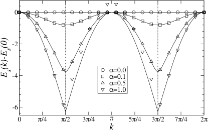
Figure 2: Lowest ED energies $E_{s}(k)-E_{s}(0)$ vs $k$ in $L=21$ chain with zero holes at $J_{z}/t=4.0$ (spinon dispersion). Solid lines show spinon dispersion for an infinite system obtained from BA.Johnson et al. (1973) All the energies are in units of $t$.

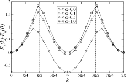
Figure 3: Lowest ED energies $E_{h}(k)-E_{h}(0)$ vs $k$ in $L=21$ chain with one hole at $J_{z}/t=4.0$ (holon dispersion). Dashed lines are guides to the eye. All the energies are in units of $t$.

II Numerical results

We have used the ED and DMRG techniques to calculate the ground state energies (GSEs) of the model for different system sizes and doping levels. This information was then used to extract the binding energy of a spinon-holon state in the infinite size limit.

In ED we start by considering a subset of states of a system of size $L$ with given total hole number $n$ and total $S^{z}$. To take advantage of the translational symmetry, we then use these to construct a basis out of eigenstates of the translation operator with a given momentum $k$. Finally, the Hamiltonian matrix in this reduced basis is constructed, and its lowest eigenvalue is calculated iteratively using the Lanczos algorithm. The implementation of every step in the procedure is described in detail in Ref. Haas, 1995. With these techniques we were able to calculate the GSEs of systems of up to 23 sites with ED. Using DMRGWhite (1992, 1993) we have calculated GSEs of systems of up to $L=128$ sites using periodic boundary conditions (PBCs), which greatly increases the numerical effort required. Up to $m=1400$ states per block were kept in the finite system method, with corrections applied to the density matrix to accelerate convergence with PBCs.White (2005)

We have carefully tested our algorithms by comparing the results of ED and DMRG for different system sizes, both with and without the hole. We have also compared the ED energies with the independent results for the GSEs of the $XXZ$ model. Medeiros and Cabrera (1991) In all cases agreement to at least 7 decimal places was achieved.

The elementary excitations of the model may be studied by looking at systems of different sizes with either no or one hole. In the case of an odd number of sites and no holes the PBCs are frustrating, corresponding to creation of a frustrated ferromagnetic link – a spinon excitation. The lowest energies for each momentum sector for a chain of 21 sites with PBC at different anisotropies are shown in Fig. 2. This gives us the spinon dispersion, which evolves from completely flat in the Ising case $\alpha=0$ to quasi-relativistic in the isotropic case $\alpha=1$. Solid lines in Fig. 2 show the exact BA result for the spinon spectrum in the $XXZ$-model:Johnson et al. (1973)

$$\omega_{q}\!=\!c\sqrt{1-\kappa^{2}\sin^{2}q}.$$ (4)

Here $c/J_{z}=K\sqrt{1-\alpha^{2}}/\pi$, and $\kappa$ is determined from the condition $\pi K^{\prime}/K=\cosh^{-1}\left(1/\alpha\right)$, where $K\equiv K(\kappa)$ and $K^{\prime}\equiv K(\sqrt{1-\kappa^{2}})$ are complete elliptic integrals of the first kind. The lowest spinon energy is attained at $q=\pm\pi/2$ for any $\alpha>0$.

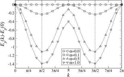
Figure 4: Lowest ED energies $E_{p}(k)-E_{p}(0)$ vs $k$ in $L=20$ chain with one hole at $J_{z}/t=4.0$ (spinon-holon pair dispersion). Dashed lines are guides to the eye.

A configuration with odd number of sites and one hole contains a “pure” holon, which can propagate through the system without disturbing the otherwise perfect AF background. Typical holon dispersions, obtained by measuring the energies of a 21-site chain with one hole, are presented in Fig. 3. The holon’s minimum energy dependence on $\alpha$ is non-trivial. At $\alpha=0$ the system has unique lowest energy point at momentum zero. This is only true for a finite system though, as in the infinite system this energy would be degenerate with the one at $k=\pi$. However, since we do not have a reciprocal space point exactly at $k=\pi$, for a finite system the energy at the momentum points closest to $k=\pi$ is somewhat higher. This mismatch is an important source of finite-size effects in our measurement, as we discuss below. As the anisotropy $\alpha$ is increased, the energy at $k=\pi$ decreases, so the ground state switches from the $k=0$ to $k=\pi$ sector at some finite intermediate value. Notably, these observations are in stark contrast with assumptions by Shiba and Ogata,Shiba and Ogata (1992) who claim that the $k=0$ and $k=\pi$ energies are going to be degenerate for any finite system in the isotropic case (they are degenerate in an infinite system though). Furthermore, their interpretation of the holon dispersion (presented in Fig. 6 of Ref. Shiba and Ogata, 1992) is somewhat misleading: they attribute the double-peaked structure of the dispersion to “strong antiferromagnetic correlations”. Our calculations confirm that the holon dispersion close to the $k=0$ and $k=\pi$ points may be very well fitted with a simple cosine dispersion of a free particle. This indicates that the characteristic double-peaked shape is formed by two different holon branches, centered at $k=0$ and $k=\pi$. As one moves away from these points towards $k=\pi/2$, the energy of the excitations grows, eventually making the creation of a spinon-antispinon pair energetically favorable, as suggested in Ref. Bernevig et al., 2002. That results in mixing of the two holon branches, which leads to a rounding of the dispersion peaks.

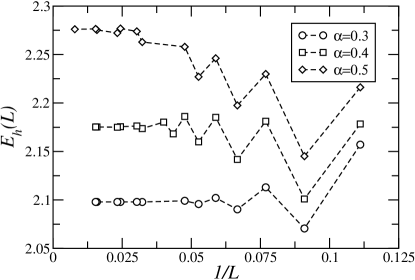
Figure 5: Raw holon GS energies for $J_{z}/t=4.0$ and different anisotropies $\alpha$ as a function of inverse system size $1/L$. Dashed lines are guides to the eye.

Finally, an even-sized system with one hole corresponds to a situation where both spinon and holon are present. The GSE as a function of $k$ for the system containing a spinon-holon pair is presented in Fig. 4.

We can measure the energies of an interacting spinon-holon pair, as well as those of individual spinon and holon excitations, by taking the GSE of a corresponding configuration and subtracting the extensive part of the energy $\tilde{\epsilon}_{\alpha}L$, where $\tilde{\epsilon}_{\alpha}$ is the energy per site of an infinite $XXZ$ chain, known from Bethe Ansatz.Yang and Yang (1966) That way we can obtain the spinon, holon, and spinon-holon pair energies for a set of different system sizes. After extrapolating to the infinite system size, the corresponding energies $E_{s}$, $E_{h}$, and $E_{p}$ can be used to calculate the binding energy of the spinon-holon state in an infinite system as

$$\Delta=E_{p}-E_{s}-E_{h}.$$ (5)

We will refer to this approach as “method $A$”.

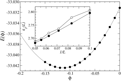
Figure 6: Ground state energy as the function of phase $\phi$ for $L=16$, $J_{z}/t=4.0$, $\alpha=0.5$. Dashed line is a quadratic fit. Inset shows the comparison of raw staggered pair energy data (open circles) and phase-corrected data (solid circles) for the same $J_{z}$ and $\alpha$, and different system sizes.

Branch	$\text{mod}(L-1,4)$	$\text{sign}(t)$
$4$-even	0	+1
	2	-1
$4$-odd	0	-1
	2	+1

Table 1: Splitting of holon energy data for different sizes $L$ and different signs of the hopping constant $t$ into the $4$-even and $4$-odd branches.

In order to obtain an accurate estimate for the excitation energies in the infinite size limit, we have to deal with a variety of finite-size effects. The lifting of degeneracy in holon dispersion mentioned above is one of them. It turns out that its effect on the resulting GSE depends on whether the system size $L$ (or $L-1$ if $L$ is odd) is divisible by 4 or not, so we will refer to these two data branches as $4$-even and $4$-odd, respectively. Such a $\textrm{mod}(4)$ dependence has been extensively discussed in the literature (see Ref. Bernevig et al., 2002 and references therein). In the $4$-even branch the energy $\epsilon_{k=0}$ provides an upper bound for the true GSE, while $\epsilon_{k=\pi}$ serves as a lower bound, and the bounds are reversed for the $4$-odd case. Another source of finite-size corrections is the incommensurability of the momentum space points in the systems of odd size. For example, it can be seen from Fig. 2 that for spinons the GS corresponds to momentum $\pi/2$ in the $L=\infty$ limit. However, for any finite-sized system with odd $L$ there will be no reciprocal space point $k=\pi/2$, instead the GSE will occur at one of the nearest points with momentum $k=\pi/2\pm\delta_{L}$, where with $\delta_{L}=\pi/L$. As the system size is increased, $\delta_{L}$ will go to zero, and the GSE will drift towards its infinite-$L$ limiting value. Similarly, we cannot directly measure the GSE for holons (Fig. 3) at $k=\pi$. All these factors lead to a highly non-trivial finite size dependence. As an example, Fig. 5 shows the size dependence of the raw holon energies. To get a meaningful extrapolation the separate analysis of $4$-even and $4$-odd branches, which contain only half of the original points, is required.

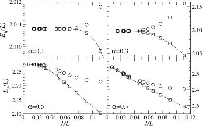
Figure 7: The $4$-even (circles) and $4$-odd (squares) branches of holon energy data for $J_{z}/t=4.0$ and different anisotropies $\alpha$. The “good” branch is used to extrapolate to $L=\infty$, using form (6) with $n=4$ and the WdV values of $\lambda$ from Ref. de Vega and Woynarovich, 1985

The situation with incommensurate $k$-space points can be improved by imposing twisted boundary conditions on the model.Zotos et al. (1990) A boundary twist leads to the translation of the points in $k$-space, but does not affect the energy spectrum. Thus, by adjusting the twist one can shift the $k$-point with anticipated minimum energy from an incommensurate location in $k$-space to an accessible one. In case of holons such a procedure is particularly simple, since we have to use a phase shift of $\pi$ to move the $k=\pi$ point of the original model to momentum $k=0$ for a model with boundary twist. Such a phase shift is readily implemented just by switching the sign of the hopping constant $t$ to the opposite one. That enabled us to reconstruct the points, lost due to the splitting into $4$-even and $4$-odd branches, by complementing the holon GSE data with measurements performed on the model with $t=-1$, as shown in Table 1.

The spinon-holon pair GSE data also suffer from the $k$-mismatch, as the GS is achieved at an incommensurate $k$-point.Zotos et al. (1990) In principle, the same procedure may be applied to improve the pair energy data. There, however, the phase shift $\phi$ needed to shift the energy minimum to an accessible momentum point is size-dependent, so it has to be determined individually for every data point. By replacing $t$ in (2) by $te^{i\phi}$ and tuning the phase shift $\phi$, we were able to measure the total energy of the system as a function of $\phi$ using ED. An example of such dependence is presented in Fig. 6. One remarkable feature of this dependence is that it is very well fit by a quadratic polynomial, so it is sufficient to know the energy at two different non-zero values of $\phi$ to recover the “true” lowest energy at the minimum with excellent accuracy. The inset of Fig. 6 shows dramatic improvement of the data due to the phase-induced correction. While such boundary conditions can be readily handled by ED, our DMRG code required extensive modifications to support them. Thus, in this work we perform the extrapolations using only the raw spinon-holon pair GSE data, split into $4$-even and $4$-odd branches. Further improvement of the precision of our results by using phase-adjusted data is possible.

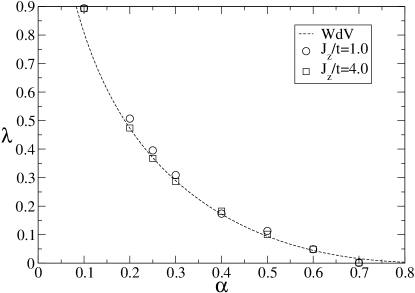
Figure 8: Comparison of the analytic values of $\lambda$ from Ref. de Vega and Woynarovich, 1985 (dashed line) with the values obtained by fitting the holon data with form (6) and keeping $\lambda$ a free fitting parameter (symbols).

After the data for holon and pair are split into such branches, we need to extrapolate them to the $L=\infty$ limit, using a reasonable fitting form. From the holon (Fig. 7) and pair (Fig. 9) excitation energy data it is evident, that it has a complicated size dependence, which cannot be adequately described by a polynomial. Clearly, at large $L$ the difference between the limiting value and the data points drops exponentially with increasing $L$. Incidentally, the size dependence for the GSE of the $XXZ$ model, deduced by Woynarovich and de Vega (WdV) from BA,de Vega and Woynarovich (1985) is also dominated by an exponential factor $\exp(-\lambda L)$. That inspired us to attempt fitting the holon and pair data with the functional form

$$E_{L}=E_{\infty}+e^{-\lambda L}P_{n}(1/L),$$ (6)

where $P_{n}(x)$ is a polynomial of order $n$ ($n\leq 4$) in $x$ with adjustable coefficients. Not only does it work remarkably well for both holons and pairs (extrapolations are shown in Fig. 7 and Fig. 9 with dashed lines), but the values of the coefficient $\lambda$ we have found by keeping this parameter free in our holon fits provide an excellent match to the analytic values found by WdV for the $XXZ$ model (their comparison is presented in Fig. 8). Therefore, we have assumed that for holons the $\lambda$ values found by WdV are either exact, or a very good approximation. Thus, we used them in our holon fits, reducing the total number of free parameters by one. For pairs the values of the $\lambda$ parameter did not correlate with WdV results at all, so it had to be kept as a free parameter in the fit.

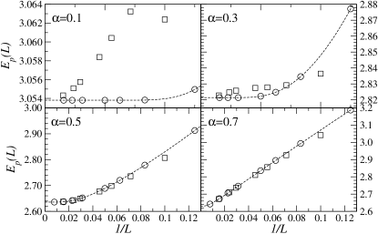
Figure 9: The $4$-even (circles) and $4$-odd (squares) branches of spinon-holon pair energy data for $J_{z}/t=4.0$ and different anisotropies $\alpha$. The “good” branch is used to extrapolate to $L=\infty$, using form (6) with $n=4$.

When the parameter $\lambda$ is sufficiently large (for $\alpha\lesssim 0.3$), the exponential factor in (6) makes the asymptotic approach to the infinite value very rapid, allowing us to simply adopt the energy value for the largest available size as the infinite-size limiting value. Increasing $\alpha$ results in decreasing $\lambda$, which pushes the onset of the exponential size dependence to larger and larger system sizes. In this regime the extrapolation using form (6) must be used. Around $\alpha\sim 0.5$ parameter $\lambda$ becomes comparable with the inverse of the maximum available system size. At higher anisotropies the onset of the exponential behavior in size dependence takes place at characteristic sizes, not accessible by our calculations (as can be seen on the lower right panel of Fig. 9), making the precise extrapolation of the pair excitation energy impossible. We can improve the accuracy of the extracted infinite size value $E_{\infty}$ by noting that both for holons and pairs one of the branches is always more “well-behaved” than the other one. For example, non-uniform behavior of the $4$-even branch for holons can be seen on the lower left panel of Fig. 7 (it peaks slightly around $1/L=0.025$), and on the upper panels of Fig. 9 for the $4$-odd pair branch. This non-uniformity of the “bad” branch usually results from the GS switching from one momentum sector to a different one as a function of $L$. In our analysis we have used only the extrapolations obtained with the “well-behaved” branch – $4$-odd for holons and $4$-even for pairs. The energy for the spinon excitations can, in principle, be extracted from the numerical data in a similar way. However, to further improve our results, we have used the analytic expression for the spinon excitation energy $E_{s}=\omega_{q=\pi/2}$, given by Eq. (4), thus eliminating the finite-size effects from the spinon GSE completely.

Branch	$\text{mod}(L,4)$	$\text{sign}(t)$ for $E^{1}_{L-1}$	$\text{sign}(t)$ for $E^{1}_{L+1}$
$B1$	0	-1	+1
$B2$	0	+1	-1
$B3$	2	-1	+1
$B4$	2	+1	-1

Table 2: Subdivision of the numerical data for $\Delta(L)$ into different branches due to finite size effects in method $B$.

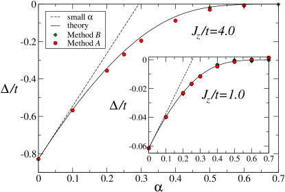
Figure 10: (Color online). Binding energy $\Delta$ as a function of $\alpha$ for $J_{z}/t=4.0$ and $J_{z}/t=1.0$ (inset). Data includes the theoretical prediction (solid line), numerical results from ED and DMRG data obtained by method $A$ (circles) and method $B$ (diamonds). Dashed line shows the linear approximation (25), valid at small $\alpha$.

Finally, the binding energy results for $L=\infty$ obtained by method $A$ using (5) for $J_{z}/t=4.0$ and $J_{z}/t=1.0$ are presented in Fig. 10. These data are of high-precision for $\alpha<0.5$. We estimate the maximum relative error of the resulting binding energy by studying the quality of the fits and the variation of $\Delta_{\infty}$ depending on the fit type. At $\alpha=0.5$ the error does not exceed 3% (10%) for $J_{z}/t=4.0$ ($J_{z}/t=1.0$) and becomes negligible very rapidly for smaller values of $\alpha$. For $\alpha=0.6$ the error is of the order of 10% (100%) for $J_{z}/t=4.0$ ($J_{z}/t=1.0$), and for $\alpha=0.7$ it exceeds $100$% for both representative values of $J_{z}$. As mentioned before, we do not consider the binding energy results for $\alpha>0.6$ to be reliable due to issues with pair energy extrapolation. Also, at larger values of $\alpha$ the value of the binding energy becomes comparable with the accuracy of our DMRG method (about $10^{-7}$ to $10^{-8}$ absolute precision, leading to about $10^{-4}t$ accuracy of the binding energy at $L=128$ and $J_{z}/t=4.0$), imposing a natural limitation on the quality of the data.

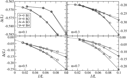
Figure 11: Size dependence for different branches of binding energy $\Delta(L)$ at $J_{z}/t=4.0$. For branch definition see Table 2. Solid lines are guides to the eye, dashed curve is the polynomial extrapolation of the “good” branch $B2$. Legend applies to all panels.

An alternative way to extrapolate the binding energy to the infinite size limit is to calculate it for every system size $L$ individually, and then do the extrapolation of the resulting size dependence to $L=\infty$. In this method (referred to as “method $B$”) we intentionally avoid using any BA results, to see whether the reliable binding energy data may be obtained based on the numerical results alone. One could hope that the finite-size effects of various components entering the binding energy may cancel out, allowing the extrapolation to the infinite-size limit using a simple polynomial in $1/L$, instead of an exponential. This approach, not depending on the theoretical results, provides an important validity test for the results of method $A$.

Since holon and spinon GSEs are only available for odd $L$, and the spinon-holon pair ones only for even $L$, we define the finite size binding energy for an even size $L$ as

$$\Delta(L)=E^{0}_{L}+E^{1}_{L}-[E^{0}_{L-1}+E^{0}_{L+1}+E^{1}_{L-1}+E^{1}_{L+1}]/2,$$ (7)

where $E^{h}_{L}$ is the ground state of a system with $L$ sites, doped with $h$ holes. This expression is analogous to (5): sum of first two terms corresponds to the pair energy, while $(E^{0}_{L-1}+E^{0}_{L+1})/2$ and $(E^{1}_{L-1}+E^{1}_{L+1})/2$ represent the average energy of a system of size $L$ with a spinon and holon, respectively. Again, due to staggering of the GSEs, binding energy data splits into a $4$-even and $4$-odd branches, depending on whether $L$ is divisible by $4$ or not. However, in this case we have an additional freedom of choosing the sign of $t$ for holon energies $E^{1}_{L-1}$ and $E^{1}_{L+1}$. Taking this into account results in 4 different data branches, defined in Table 2. The remaining possibilities of using the same sign of $t$ both for $E^{1}_{L-1}$ and $E^{1}_{L+1}$ have been discarded as obviously suboptimal.

The size dependence of different data branches for different anisotropies is presented in Fig. 11. Due to splitting, the number of points in each branch is pretty small, so we have used a polynomial of maximum possible degree (one less than the number of points) to perform the extrapolation to the infinite system size. From our previous experience we know that the “good” holon branch in method $A$ corresponds to branch $B2$, therefore we used the extrapolated value from this branch as our final result for the binding energy. As can be seen in Fig. 10, the data from methods $A$ and $B$ are in excellent agreement in the range of $\alpha$, where its calculation is reliable. However, we have found that the method $B$ data always has a larger relative error than method $A$, mainly due to the size-dependence of the spinon component, eliminated in method $A$.

III Theoretical results

Because in the Ising limit the spinon is impurity-like, the spinon-holon binding at $\alpha=0$ can be solved in a number of ways (see Appendix) to give Eq. (3). For finite $\alpha$ the binding energy of the spinon-holon state may be calculated analytically by finding the poles of the two-particle scattering amplitude $\Gamma$. We will use shorthand notation ${\mathbf{q}}=(q,\omega)$ and ${\mathbf{k}}=(k,\epsilon)$ to denote the momenta and energies of spinon and holon, respectively.

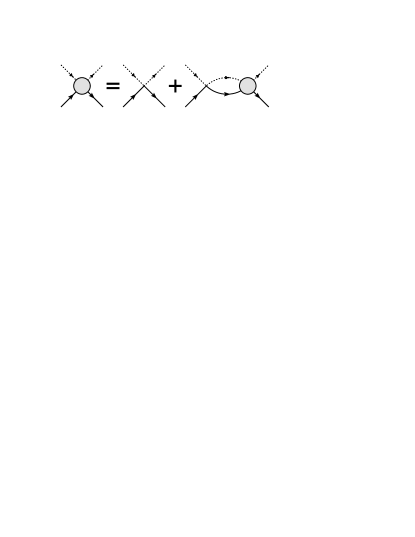
Figure 12: Bethe-Salpeter equation for the spinon-holon scattering amplitude (circle). Spinons (holons) are shown by dashed (solid) lines.

Scattering amplitude $\Gamma$ obeys the Bethe-Salpeter equation,Berestetskii et al. (1982) presented in diagrammatic form in Fig. 12. Generally, it depends on both the incoming ${\mathbf{q}}$, ${\mathbf{k}}$ and outgoing $\bar{{\mathbf{q}}}$, $\bar{{\mathbf{k}}}$ $2$-momenta of spinon and holon. Using that momentum and energy are conserved, ${\mathbf{k}}+{\mathbf{q}}=\bar{{\mathbf{k}}}+\bar{{\mathbf{q}}}={\mathbf{P}}\equiv(P,E)$, we may write it as

$$\Gamma_{{\mathbf{P}}}({\mathbf{q}},\bar{{\mathbf{q}}})=V_{q,\bar{q}}+\int_{{\mathbf{q}}^{\prime}}V_{q,q^{\prime}}G^{s}_{{\mathbf{q}}^{\prime}}G^{h}_{{\mathbf{P}}-{\mathbf{q}}^{\prime}}\Gamma_{{\mathbf{P}}}({\mathbf{q}}^{\prime},\bar{{\mathbf{q}}}).$$ (8)

Here $V_{q,q^{\prime}}$ is the spinon-holon interaction, and $G^{h(s)}$ is the holon (spinon) Green’s function. A shorthand notation $\int_{{\mathbf{q}}^{\prime}}\equiv\int_{-\infty}^{\infty}\,\frac{d\omega^{\prime}}{2\pi}\,\sum_{q^{\prime}}$, with $\sum_{q^{\prime}}=\int_{-\pi}^{\pi}\frac{dq^{\prime}}{2\pi}$ is used. In the vicinity of the pole of $\Gamma$, Eq. (8) should reduce to a homogeneous integral equation with $\Gamma$ whose dependence on one of the momenta $\bar{{\mathbf{q}}}$ is only parametric and can be droppedBerestetskii et al. (1982)

$$\Gamma_{{\mathbf{P}}}({\mathbf{q}})=\int_{{\mathbf{q}}^{\prime}}\,V_{q,q^{\prime}}G^{s}_{{\mathbf{q}}^{\prime}}G^{h}_{{\mathbf{P}}-{\mathbf{q}}^{\prime}}\Gamma_{{\mathbf{P}}}({\mathbf{q}}^{\prime}).$$ (9)

The holon and spinon create a bound state if this integral equation has a solution. By introducing a function

$$\chi_{{\mathbf{P}}}(q)=\int_{\omega}G^{s}_{{\mathbf{q}}}G^{h}_{{\mathbf{P}}-{\mathbf{q}}}\Gamma_{{\mathbf{P}}}({\mathbf{q}}),$$ (10)

multiplying both sides of (9) by $G^{s}_{{\mathbf{q}}}G^{h}_{{\mathbf{P}}-{\mathbf{q}}}$, and integrating over $\omega$, we arrive at

$$\chi_{{\mathbf{P}}}(q)=\left[\int_{\omega}G^{s}_{{\mathbf{q}}}G^{h}_{{\mathbf{P}}-{\mathbf{q}}}\right]\sum_{q^{\prime}}V_{q,q^{\prime}}\chi_{{\mathbf{P}}}(q^{\prime}).$$ (11)

Evaluation of the first integral on the rhs requires knowledge of the spinon and holon Green’s functions. For now we will just assume that they are free particles with some dispersions $\omega_{q}$ and $\epsilon_{k}$, the specific form of which is to be determined:

$$G^{s}_{q,\omega} = \frac{1}{\omega-\omega_{q}+i\delta},$$

$$G^{h}_{k,\epsilon} = \frac{1}{\epsilon-\epsilon_{k}+i\delta}.$$

With this assumption the integral is trivially done, yielding the final form of the Bethe-Salpeter equation for $\chi_{{\mathbf{P}}}(q)$:

$$\chi_{{\mathbf{P}}}(q)=\frac{1}{E-\epsilon_{P-q}-\omega_{q}}\sum_{q^{\prime}}V_{q,q^{\prime}}\chi_{{\mathbf{P}}}(q^{\prime}).$$ (12)

From this equation it is clear that $\chi_{{\mathbf{P}}}(q)$ is nothing but the pair wavefunction and the equation (12) is the Schrödinger equation for it in integral form. The pair energy $E$ may be thought of as the binding energy $\Delta$, measured relative to the lowest energies of the particles $\epsilon_{0}=min[\epsilon_{k}]$ and $\omega_{0}=min[\omega_{q}]$:

$$E=\Delta+\epsilon_{0}+\omega_{0}.$$ (13)

In the Ising limit $\epsilon_{k}=-2t\cos k$, $\epsilon_{0}=-2t$, $\omega_{q}\!=\!\omega_{0}\!=\!J_{z}/2$, and $V_{q,q^{\prime}}=-\omega_{0}$, so Eq. (12) is readily solved by

$$\chi_{{\mathbf{P}}}(q)=\frac{C}{E-\epsilon_{P-q}-\omega_{0}},$$ (14)

yielding a dispersionless ($P$-independent) bound state with $\Delta$ given by (3). From general considerations, the binding energy in 1D should scale as $-V^{2}m$, where $V$ is interaction strength and $m$ is the particle mass. In the Ising case this gives $\Delta\!\sim\!-J_{z}^{2}/t$, in agreement with the exact result (3).

Away from the Ising limit (at nonzero $\alpha$) the physical picture changes qualitatively. First of all, due to the spin-flips the spinon is no longer stationary; it may propagate through the lattice and has a $\pm\pi/2$ momentum in the ground state. Second, the spinon-holon interaction $V_{q,q^{\prime}}$ changes. Finally, the holon dispersion is altered as well and may acquire some “dressing”. The changes in the latter, however, should not affect the pairing in any significant way due to the fact that only the holon dispersion near the energy minimum matters for it. The holon mass renormalization has been analyzed in detail in Ref. Zotos et al., 1990 and it was found insignificant throughout the anisotropic regime $0\leq\alpha\leq 1$. This means that both the “dressing” and the holon dispersion changes are minor and should not affect pairing. On the other hand, changes in the spinon dispersion are qualitative and drastic. At $\alpha=0$, the spinon may be viewed as a gapped, immobile excitation with the energy $\omega_{q}\!=J_{z}/2$. With increasing $\alpha$ it evolves into a relativistic one, turning completely gapless in the isotropic limit $\alpha=1$, where its dispersion is $\omega_{q}=J_{z}(\pi/2)|\cos q|$. The spinon dispersion for the $XXZ$ model at intermediate values of $\alpha$, shown by solid lines in Fig. 2, is known exactly from BA,Johnson et al. (1973) see Eq. (4). While the parameter $c/J_{z}$ in this equation changes almost linearly between $1/2$ and $\pi/2$ as $\alpha$ goes from $0$ to $1$, the parameter $\kappa$ varies from $0$ to $1$ rather steeply, achieving the value of approximately $0.996$ at $\alpha=0.5$. As a result, the spinon gap $\omega_{s}$ given by $\omega_{s}=c\sqrt{1-\kappa^{2}}$ becomes sufficiently small already at $\alpha\sim 0.5$. One can obtain the asymptotic behavior for $\omega_{s}$, valid for $\alpha\gtrsim 0.5$, and show that it approaches zero exponentially in $(1-\alpha)^{-1/2}$ as $\alpha\rightarrow 1$:

$$\omega_{s}\approx 4c\exp\left(-\pi^{2}\sqrt{\frac{\alpha}{8(1-\alpha)}}\right).$$ (15)

The smallness of the spinon gap may be used to write the spinon spectrum in approximate “quasi-relativistic” form in this regime:

$$\omega_{q}=\sqrt{c^{2}\left(q-\frac{\pi}{2}\right)^{2}+\omega_{s}^{2}}.$$ (16)

Another effect of increasing $\alpha$ is a dramatic decrease of the spinon’s effective mass

$$m=\left.\left(\frac{\partial^{2}\omega_{q}}{\partial q^{2}}\right)^{-1}\right|_{q=\pi/2}$$ (17)

which goes from $(4\alpha J_{z})^{-1}$ at $\alpha\ll 1$ to $\omega_{s}/c^{2}$ at $\alpha\gtrsim 0.5$. Such a change can be observed in the spectra in Fig. 2, where increasing $\alpha$ makes the energy minimum into a sharp tip, indicating the mass reduction. Thus, even without knowing a specific form of interaction, one can anticipate that the spinon-holon binding will be strongly affected by such changes in the spinon spectrum. We also note that since the spinon becomes much lighter than the holon, $m_{s}\ll\!m_{h}\!\simeq\!(2t)^{-1}$, the role of the holon dispersion in (12) becomes secondary close to the isotropic limit.

The remaining question is that of the spinon-holon interaction. One can analyze the binding problem in the small-$\alpha$ limit rigorously. The changes to the holon and the AF GSEs are of order $O(\alpha^{2})$, while the spinon energy changes in the order $O(\alpha)$:

$$\omega_{q}=\omega^{0}+\delta\omega_{q}=J_{z}/2+\alpha J_{z}\cos 2q.$$ (18)

One of the consequences of non-zero anisotropy is the $\pm\pi/2$ momentum of the GS of the spinon. This immediately implies that the spinon-holon pairing should result in a bound state with finite total momentum $P\!=\!\pm\pi/2$, in agreement with the numerical data, shown in Fig. 4. Since the energy of the system is lowered when the AF domain walls associated with the spinon and holon pass through each other, the interaction between the two can be written as a “contact” attraction of the strength $V^{0}\!=\!-J_{z}/2$. Using real-space considerations we find that this leads to a direct relation between interaction in the momentum space and spinon dispersion. To the order $O(\alpha)$ the interaction can be shown to be:

$$V_{q,q^{\prime}}\!=\!-\omega^{0}\!-\!(\delta\omega_{q}\!+\!\delta\omega_{q^{\prime}})/2.$$ (19)

This equation may be used to derive an analytic expression for the binding energy $\Delta$, exact to the first order in $\alpha$. Substituting (19) into (12) we get

$$\chi_{{\mathbf{P}}}(q)=-\frac{1}{E_{q}}\left[A\left(\omega^{0}+\frac{\delta\omega_{q}}{2}\right)+\frac{B}{2}\right],$$ (20)

where

$$A = \sum_{q^{\prime}}\chi_{{\mathbf{P}}}(q^{\prime}),$$ (21)

$$B = \sum_{q^{\prime}}\delta\omega_{q^{\prime}}\chi_{{\mathbf{P}}}(q^{\prime}),$$ (22)

$$E_{q} \equiv E-\epsilon_{P-q}-\omega_{q}.$$ (23)

After inserting this result for $\chi(q)$ into (12), dropping the higher-order terms in $\alpha$, and some algebraic manipulations, we end up with the following equation for $\Delta$:

$$1=-\frac{J_{z}}{2}\sum_{q}\frac{1+2\alpha\cos 2q}{\Delta-(\epsilon_{P-q}-\epsilon_{0})-2\alpha(\cos 2q+1)}.$$ (24)

Further expansion in $\alpha$ and calculation using the “bare” holon energy $\epsilon_{k}=\epsilon^{0}_{k}\equiv 2t\cos k$, yields an expression for $\Delta$ which is valid to order $O(\alpha)$:

$$\Delta=\!\Delta_{0}(1-C\alpha),$$ (25)

with $\Delta_{0}$ given by Eq. (3) and

$$C=\frac{2J_{z}^{2}}{\sqrt{16t^{2}+J_{z}^{2}}\left(\sqrt{16t^{2}+J_{z}^{2}}-4t\right)}.$$ (26)

Interestingly, the initial slope of $\Delta(\alpha)/\Delta(0)$ depends only weakly on the value of $J_{z}$: it is bound between $C=4$ at $J_{z}=0$ and $C=2$ at $J_{z}/t\gg 1$ and varies smoothly between them. This linear-$\alpha$ result (25) is shown in Fig. 10 with dashed lines. It is in extremely close agreement with the numerical data in the small-$\alpha$ regime.

Having established the form (19) of the spinon-holon interaction for small $\alpha$, we can now try to address the question of how might the general form of the interaction, valid for any anisotropy $\alpha$, look like. While there are no strict analytical arguments for it, we may formulate a number of criteria, which this form must satisfy. First of all, the interaction $V_{q,q^{\prime}}$ must be symmetric with respect to momenta, $V_{q,q^{\prime}}=V_{q^{\prime},q}$. Second, it must reproduce the small $\alpha$ limit (19) as $\alpha\rightarrow 0$. One can also anticipate that it should be straightforwardly related to the spinon energy, similar to Eq. (19).

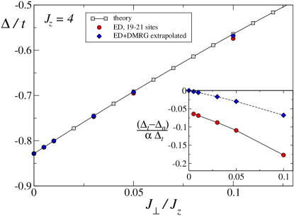
Figure 13: (Color online). Analytic ($\Delta_{t}$) and numerical ($\Delta_{n})$ results for the binding energy at small values of $\alpha$ for $J_{z}/t=4.0$. Inset shows the relative difference between the theoretical and numerical results.

Based on these requirements, we propose the following form of the interaction in the momentum space:

$$V_{q,q^{\prime}}=-\sqrt{\omega_{q}\omega_{q^{\prime}}}.$$ (27)

This is somewhat reminiscent of the electron-phonon interaction that is proportional to square-root of the phonon energy. Using this Ansatz for $V_{q,q^{\prime}}$, spinon energy from BA, and neglecting the changes in the holon dispersion ($\epsilon_{k}\!=\!\epsilon^{0}_{k}$) we arrive at a solution of Eq. (12) of the form

$$\chi(q)=\textrm{const}\times\frac{\sqrt{\omega_{q}}}{E_{q}},$$ (28)

leading to the following equation for $\Delta$:

$$1=-\sum_{q}\frac{\omega_{q}}{\Delta-(\epsilon_{P-q}-\epsilon_{0})-(\omega_{q}-\omega_{0})}.$$ (29)

Solving this equation numerically yields the complete dependence of the binding energy $\Delta$ on anisotropy $\alpha$ shown as solid lines in Fig. 10. Not only this equation naturally yields our small-$\alpha$ results, but it also provides a very close agreement with the numerical data for all values of $J_{z}$ and for all $\alpha$ we can access numerically. This provides a very convincing a posteriori verification of our spinon-holon interaction Ansatz.

Since we neglect the changes in the holon dispersion, the deviation of our theoretical result for $\Delta$ from an exact answer is expected to occur in order $O(\alpha^{2})$. We verified that in the small-$\alpha$ limit. Results of the comparison of analytic and numerical results are presented in Fig. 13. At $\alpha=0$, numerical data obtained using method $B$ for the largest system size accessible by ED ($19$-$21$ sites) agrees with the exact analytical result (3) within the numerical precision ($10^{-7}t$). However, any small anisotropy results in a finite-size effect, linear in $\alpha$ (see inset of Fig. 13). This may be understood in terms of the momentum space mismatch, discussed earlier: for any finite $\alpha$ and finite size $L$ we cannot obtain the “true” GSE value for spinon from the numerical simulations, because the momentum point corresponding to its lowest energy ($q=\pi/2$) is incommensurate with the available momentum points. Thus, a finite-size effect of the order $O(1/L)$ is expected for any finite $\alpha$. The extrapolated data, on the other hand, displays the expected $O(\alpha^{2})$ deviation.

Although we have no formal proof of the validity of our interaction Ansatz for all $\alpha$, the agreement with the numerical data makes it very plausible. As the binding energy becomes small, it is the long-wavelength features of the dispersions and interaction that determine the pairing. One can see from Eq. (27) that at $\alpha\!\rightarrow\!1$ the characteristic interaction at low energies is $V\!\approx\!\omega_{s}$. Thus, within the qualitative picture of pairing in 1D, both the interaction and the spinon mass become proportional to the spinon gap $\omega_{s}$ that tends to zero exponentially. One then expects the asymptotic behavior $\Delta\sim-V^{2}m\sim-\omega_{s}^{3}$. From Eq. (29) we can derive such an asymptotic expression explicitly: $\Delta\approx{\cal D}(J_{z},\alpha)\omega_{s}^{3}/c^{2}$, where

$${\cal D}(J_{z},\alpha)=\left\{\begin{array}[]{ll}1,&t\gg J_{z};\\ {\displaystyle\frac{1}{2}\left(\frac{\pi c}{4t\ln(c/2t)}\right)^{2}},&t\ll J_{z}.\end{array}\right.$$ (30)

Notably, the exponential behavior of the binding energy is determined solely by the asymptotic behavior (15) of the spinon gap $\omega_{s}$, with the expression in the exponential dependent only on $\alpha$ and not on $J_{z}/t$. Thus, the holon energy scale is secondary as it only enters the prefactor. Altogether, this explains the quick (exponential) drop-off

$$\Delta\sim-\exp\left(-3\pi^{2}\sqrt{\frac{\alpha}{8(1-\alpha)}}\right)$$ (31)

already at intermediate values of $\alpha\gtrsim 0.5$.

From this asymptotic expression and Eq. (29) one can see that the binding energy vanishes in the isotropic limit together with the spinon gap. Thus, our spinon-holon interaction Ansatz also provides a natural and simple explanation of the non-zero binding at finite $q$ but no bound state at $\alpha=1$. This is possible because the interaction of the holon with the long-wavelength spinon $V_{q,q^{\prime}}$ vanishes together with the spinon energy. Then, the pairing is not strong enough to produce a bound state in the isotropic limit. We also find that in the isotropic limit the spinon-holon pair wave-function, Eq. (28), is $\chi(q)\sim 1/\sqrt{\omega_{q}}$. In real space, this would correspond to $1/\sqrt{r}$ spinon-holon correlation, exactly the behavior found in Ref. Bernevig et al., 2002.

IV Conclusions

We have performed extensive analytical and numerical studies of an anisotropic version of the $t$-$J$ model, doped with a single hole. Our main result is that the anisotropy of the spin-spin interaction leads to an effective attraction between the spinon and holon excitations, resulting in existence of a spinon-holon bound state. Using the ED and DMRG techniques we have numerically estimated the binding energy as a function of anisotropy. We have described in detail the finite-size effects which arise due to various factors and, by examining various ways to mitigate or eliminate them, worked out a procedure for extrapolation of the finite-size data to the infinite size limit, resulting in precise estimates of the binding energy up to anisotropy $\alpha=0.5$. The resulting numerical values have been found to be in excellent agreement with the theory, based on Bethe-Salpeter equation. Using the experience gained while studying the small anisotropy limit, we have formulated the criteria for the form of the spinon-holon interaction in momentum space, and proposed a form (27) for it, which results in excellent agreement of analytical and numerical results. Finally, we have identified the changes in the spinon spectra as the primary factor affecting the behavior of the binding energy as a function of anisotropy. We have demonstrated that the binding energy goes to zero exponentially, as a power of the spinon gap, when isotropic limit is approached. This behavior also explains why there is no spinon-holon binding in the isotropic $t$-$J$ model. These results could be tested in photoemission experiments in 1D spin-chain systems with Ising anisotropies.

We would like to note that the problem we have considered is strictly single hole, and its extension to the finite-doping case is not trivial. For instance, even in the pure Ising limit one could deliberately avoid creating any spinons by putting an even number of holes in the holon-only states (see Ref. Batista and Ortiz, 2000). However, if spinons are present in the system, the interaction between them and the holons remains attractive even at a finite hole doping and may lead to their binding.

V Acknowledgments.

We would like to thank A. Bernevig and O. Starykh for fruitful discussions. This work was supported in part by DOE grant DE-FG02-04ER46174 and by a Research Corporation Award (JŠ and AC) and by NSF grant DMR-0605444 (SRW).

Appendix A Different treatments of the $\alpha=0$ problem

For pedagogical purposes we describe three different analytic ways to determine the bound state energy of the $t$-$J_{z}$ model, doped with a single hole.

Method 1. The first method we discuss is the exact calculation of the hole’s real-space Green’s function. It can be accomplished using the expansion in paths,Nagaoka (1965); Brinkman and Rice (1970) or the recursion techniqueStarykh and Reiter (1996); Chernyshev and Leung (1999) that is also identical to the Lanczos method. We use the latter as the most straightforward. The bound state energy may be determined as the pole of the diagonal element

$$G_{ii}(\omega)=\left\langle\psi_{i}\left|\frac{1}{\omega-{\mathcal{H}}}\right|\psi_{i}\right\rangle,$$ (32)

where $\psi_{i}$ is the state of the system in which the hole is located at site $i$. It may be calculated exactly by noting that we may bring the Hamiltonian to a tridiagonal form by generating a basis

$$|n+1\rangle=H|n\rangle-a_{n}|n\rangle-b_{n}^{2}|n-1\rangle,$$ (33)

where

$$a_{n}=\frac{\langle n|{\mathcal{H}}|n\rangle}{\langle n|n\rangle},\quad b_{n}^{2}=\frac{\langle n|n\rangle}{\langle n-1|n-1\rangle}.$$ (34)

It is easy to see that in this basis the diagonal Green’s function may be represented as a continued fraction:

$$G_{11}(\omega)=\left\langle 1\left|\frac{1}{\omega-{\mathcal{H}}}\right|1\right\rangle=\frac{b_{1}^{2}}{\omega-a_{1}-\frac{b_{2}^{2}}{\omega-a_{2}-\ldots}}.$$ (35)

In the case of the $t$-$J_{z}$ model the coefficients in the continued fraction have the form

$$b_{1}^{2} = 1$$

$$b_{2}^{2} = 2t^{2}$$

$$b_{3}^{2} = b_{4}^{2}=b_{5}^{2}=\ldots=t^{2}$$ (36)

and

$$a_{1} = -\omega^{0}\equiv-J_{z}/2$$

$$a_{2} = a_{3}=a_{4}=\ldots=0.$$ (37)

Thus, we may rewrite (35) as

$$G_{ii}(\omega)=\frac{1}{\omega+\omega^{0}-2\Sigma(\omega)},$$ (38)

where

$$\Sigma(\omega)=\frac{t^{2}}{\omega-\frac{t^{2}}{\omega-\ldots}}=\frac{t^{2}}{\omega-\Sigma_{(}\omega)}.$$ (39)

Solving for $\Sigma(\omega)$ yields the Green’s function

$$G(\omega)=\frac{1}{J_{z}/2\mp\sqrt{\omega^{2}-4t^{2}}},$$ (40)

with poles given by

$$\bar{\omega}=\pm\sqrt{4t^{2}+J_{z}^{2}/4}.$$ (41)

The energy corresponding to the lowest pole is lower than hole’s kinetic energy $-2t$, indicating the presence of a bound state. The expression for the binding energy $\Delta=2t-|\bar{\omega}|$ is equivalent to (3). The quasiparticle residue of that pole is given by:Sorella and Parola (1998)

$$Z=\frac{J_{z}}{2|\bar{\omega}|}=\frac{J_{z}}{\sqrt{16t^{2}+J_{z}^{2}}}.$$ (42)

At large $t/J_{z}$, in agreement with the naive expectations, $Z\approx(J_{z}/2)/2t$, the ratio of spinon-holon interaction strength to the holon kinetic energy.

Method 2. Another approach is to consider the immobile spinon to be an impurity and solve the problem of a freely moving hole scattering on it using the $T$-matrix formalism. To that end we write the Hamiltonian of the hole as

$${\mathcal{H}}_{0}=-2t\sum_{k}\cos(k)c^{\dagger}_{k}c_{k},$$ (43)

where $c_{k}$ is the annihilation operator for a hole with momentum $k$. The impurity Hamiltonian may be written as

$${\mathcal{H}}^{\prime}=-\omega^{0}c^{\dagger}_{r}c_{r},$$ (44)

i.e. it lowers the energy by $\omega^{0}\equiv J_{z}/2$ if the hole is present at the origin site. Transforming it to the momentum space after assuming $r=0$ yields

$${\mathcal{H}}^{\prime}=-\omega^{0}\sum_{k,k^{\prime}}c^{\dagger}_{k}c_{k^{\prime}}.$$ (45)

The impurity Hamiltonian is such that each of its matrix elements is equal to $-\omega^{0}$. The equation for $T$-matrix is

$$T={\mathcal{H}}^{\prime}+{\mathcal{H}}^{\prime}G_{0}T.$$ (46)

Inserting complete sets of states and using the fact that $G_{0}$ is diagonal and $\langle k|{\mathcal{H}}^{\prime}|k^{\prime}\rangle=-\omega^{0}$ for arbitrary $k$, $k^{\prime}$, we get the following equation for the matrix elements:

$$\langle k|T|k^{\prime}\rangle=-\omega^{0}-\omega^{0}\sum_{p}\langle p|G_{0}|p\rangle\langle p|T|k^{\prime}\rangle.$$ (47)

Close examination of this expression reveals that the $T$-matrix is independent of $k$ and $k^{\prime}$. Denoting the matrix element by $T(\omega)$ we obtain

$$T(\omega)=-\omega^{0}\left(1+T(\omega)\sum_{p}\langle p|G_{0}(\omega)|p\rangle\right).$$ (48)

The integral on the rhs

$$S=\sum_{p}\langle p|G_{0}(\omega)|p\rangle$$ (49)

can be calculated using elementary methods to find

$$S=\frac{1}{\sqrt{\omega^{2}-4t^{2}}}.$$ (50)

Thus

$$T(\omega)=-\frac{\omega^{0}\sqrt{\omega^{2}-4t^{2}}}{\omega^{0}+\sqrt{\omega^{2}-4t^{2}}}$$ (51)

The exact Green’s function of a particle with a scatterer is a function of incoming and outgoing momenta $k$ and $k^{\prime}$, given by

$$G(k,k^{\prime})=G_{0}(k)+G_{0}(k)TG_{0}(k^{\prime}).$$ (52)

This yields the following matrix element:

$$\langle k|G(\omega)|k^{\prime}\rangle=\frac{1}{\omega+2t\cos k}\left[\delta_{k,k^{\prime}}+T(\omega)\frac{1}{\omega+2t\cos k^{\prime}}\right].$$ (53)

Transforming to real space by integrating over momenta $k$ and $k^{\prime}$, we get the diagonal Green’s function at the point of origin:

$$G_{rr}(\omega) = \sum_{k,k^{\prime}}\langle k|G(\omega)|k^{\prime}\rangle$$ (54)

$$= \frac{1}{\sqrt{\omega^{2}-4t^{2}}}+\frac{1}{\omega^{2}-4t^{2}}T(\omega)$$

$$= \frac{1}{\omega^{0}+\sqrt{\omega^{2}-4t^{2}}}$$

that is equivalent to (40). This Green’s function has the poles at the locations given by (41), so it yields binding energy equivalent to (3).

Method 3. Finally, the last approach is based on the physical picture of hole decay into a spinon and holon, confined to two half-spaces (see Fig. 1), and solving the Dyson’s equation for such a decay exactly. The Dyson equation for the hole at origin has the form

$$G(\omega)=\frac{1}{(G^{0})^{-1}-\Sigma(\omega)},$$ (55)

where

$$G^{0}(\omega)=\frac{1}{\omega},$$ (56)

and self-energy $\Sigma(\omega)$ may be written in terms of the spinon Green’s function $D(\omega)$ and the holon Green’s function in a half-space $G^{(1/2)}_{h}(\omega)$:

$$\Sigma(\omega)=2t^{2}\int\,\frac{d\omega^{\prime}}{2\pi}D(\omega^{\prime})G^{(1/2)}_{h}(\omega-\omega^{\prime}).$$ (57)

Since

$$D(\omega)=\frac{1}{\omega-\omega^{0}},$$ (58)

the integral is readily done, leading to the expression for self-energy

$$\Sigma(\omega)=2t^{2}G^{(1/2)}_{h}(\omega-\omega^{0}).$$ (59)

The Green’s function (55) can then be written in terms of the shifted frequency $\tilde{\omega}=\omega-\omega^{0}$ as

$$G(\tilde{\omega})=\frac{1}{\tilde{\omega}+\omega^{0}-\Sigma(\tilde{\omega})}.$$ (60)

To calculate $G_{h}^{(1/2)}(\tilde{\omega})$, that is the Green’s function of a free hole subject to a “hard-wall” boundary condition at the origin, we note that it can be expressed as the antisymmetric part of the hole’s Green’s function $G_{h}(\omega)$ in the entire space. For example, in the coordinate representation we obtain:

$$G_{h}^{(1/2)}(x,x^{\prime};\omega)=G_{h}(x,x^{\prime};\omega)-G_{h}(x,-x^{\prime};\omega).$$ (61)

Here $G_{h}(x,x^{\prime};\omega)$ is just an inverse Fourier transform of the Green’s function of a free hole:

$$G_{h}(x,x^{\prime};\omega)=\int\frac{dp}{2\pi}\frac{e^{i(x-x^{\prime})p}}{\omega+2t\cos p}.$$ (62)

It depends only on the difference of the coordinates $x-x^{\prime}$, as expected for a translationally invariant system. We are interested in the diagonal matrix element of (61):

$$G_{h}^{(1/2)}(x;\omega) \equiv G_{h}^{(1/2)}(x,x;\omega)=$$ (63)

$$= G_{h}(x-x;\omega)-G_{h}(x+x;\omega).$$

Using (62) it may be readily found to be

$$2G_{h}^{(1/2)}(\omega)=\omega\pm\sqrt{\omega^{2}-4t^{2}},$$ (64)

again leading to the expression for $G(\omega)$ equivalent to Eqs. (40) and (54) and expression for $\Delta$, equivalent to (3).

References

- Giamarchi (2004) T. Giamarchi, Quantum Physics in One Dimension, vol. 121 of International Series of Monographs on Physics (Oxford University Press, 2004).
- Lieb and Wu (1968) E. H. Lieb and F. Y. Wu, Phys. Rev. Lett. 20, 1445 (1968).
- Shiba and Ogata (1992) H. Shiba and M. Ogata, Prog. Theor. Phys. Supp. 108, 265 (1992).
- Sorella and Parola (1998) S. Sorella and A. Parola, Phys. Rev. B 57, 6444 (1998).
- Brunner et al. (2000) M. Brunner, F. F. Assaad, and A. Muramatsu, Eur. Phys. J. B 16, 209 (2000).
- Bernevig et al. (2002) B. A. Bernevig, D. Giuliano, and R. B. Laughlin, Phys. Rev. B 65, 195112 (2002).
- Bares et al. (1991) P.-A. Bares, G. Blatter, and M. Ogata, Phys. Rev. B 44, 130 (1991).
- Nagler et al. (1983) S. E. Nagler, W. J. L. Buyers, R. L. Armstrong, and B. Briat, Phys. Rev. B 27, 1784 (1983).
- Kim et al. (1996) C. Kim, A. Y. Matsuura, Z. X. Shen, N. Motoyama, H. Eisaki, S. Uchida, T. Tohyama, and S. Maekawa, Phys. Rev. Lett. 77, 4054 (1996).
- Šmakov et al. (2007) J. Šmakov, A. L. Chernyshev, and S. R. White, Phys. Rev. Lett. 98, 266401 (2007).
- Johnson et al. (1973) J. D. Johnson, S. Krinsky, and B. M. McCoy, Phys. Rev. A 8, 2526 (1973).
- Haas (1995) S. Haas, Ph.D. thesis, Florida State University (1995), URL http://physics.usc.edu/~shaas/haasthesis.pdf.
- White (1992) S. R. White, Phys. Rev. Lett. 69, 2863 (1992).
- White (1993) S. R. White, Phys. Rev. B. 48, 10345 (1993).
- White (2005) S. R. White, Phys. Rev. B. 72, 180403 (2005).
- Medeiros and Cabrera (1991) D. Medeiros and G. G. Cabrera, Phys. Rev. B 44, 848 (1991).
- Yang and Yang (1966) C. N. Yang and C. P. Yang, Phys. Rev. 150, 321 (1966).
- de Vega and Woynarovich (1985) H. J. de Vega and F. Woynarovich, Nucl. Phys. B 251, 439 (1985).
- Zotos et al. (1990) X. Zotos, P. Prelovek, and I. Sega, Phys. Rev. B 42, 8445 (1990).
- Berestetskii et al. (1982) V. B. Berestetskii, E. M. Lifshitz, and L. P. Pitaevskii, Quantum Electrodynamics, vol. 4 of Landau and Lifshitz Course of Theoretical Physics (Pergamon Press, 1982).
- Batista and Ortiz (2000) C. D. Batista and G. Ortiz, Phys. Rev. Lett. 85, 4755 (2000).
- Nagaoka (1965) Y. Nagaoka, Sol. State Comm. 3, 409 (1965).
- Brinkman and Rice (1970) W. F. Brinkman and T. M. Rice, Phys. Rev. B 2, 1324 (1970).
- Starykh and Reiter (1996) O. A. Starykh and G. F. Reiter, Phys. Rev. B 53, 2517 (1996).
- Chernyshev and Leung (1999) A. L. Chernyshev and P. W. Leung, Phys. Rev. B. 60, 1592 (1999).