The photospheric environment of a solar pore with light bridge

Abstract

Context. Pores are one of the various features forming in the photosphere by the emergence of magnetic field onto the solar surface. They lie at the border between tiny magnetic elements and larger sunspots. Light bridges, in such structures, are bright features separating umbral areas in two or more irregular regions. Commonly, light bridges indicate that a the merging of magnetic regions or, conversely, the breakup of the area is underway:

Aims. We investigate the velocity structure of a solar pore (AR10812) with light bridge, and of the quiet solar photosphere nearby, analyzing high spatial and spectral resolution images.

Methods. The pore area has been observed with the Interferometric BI-dimensional Spectrometer (IBIS) at the Dunn Solar Telescope, acquiring monochromatic images in the Ca II 854.2 nm line and in the Fe I 709.0 nm line as well as G-band and broad-band images. We also computed the Line of Sight (LoS) velocity field associated to the Fe I and Fe II photospheric lines.

Results. The amplitude of the LoS velocity fluctuations, inside the pore, is smaller than that observed in the quiet granulation near the active region. We computed the azimuthal average LoS velocity and derived its radial profile. The whole pore is characterized by a downward velocity $\simeq-200\leavevmode\nobreak\ m\cdot s^{-1}$ and by an annular downflow structure with an average velocity of $\simeq-350\leavevmode\nobreak\ m\cdot s^{-1}$ with respect to the nearby quiet sun.
The light bridge inside the pore, when observed in the broad-band channel of IBIS and in the red wing of Ca II 854.2 nm line, shows an elongated dark structure running along its axis, that we explain with a semi-analytical model. In the highest resolution LoS velocity images the light bridge shows a profile consistent with a convective roll: a weak upflow, $\sim 50\div 100\leavevmode\nobreak\ m\cdot s^{-1}$, in correspondence of the dark lane, flanked by a downflow, $\sim-(200\div 300)\leavevmode\nobreak\ m\cdot s^{-1}$.

1 Introduction

The inhomogeneous and structured aspect of the solar photosphere essentially originates from convective flows, carrying energy from the deeper layers of the star, and from the magnetic field, emerging at the surface. The photosphere shows a wide variety of magnetic features, ranging from the largest sunspots, with typical field strengths of $\simeq 3000$ G, down to the 0.1 Mm scale magnetic elements, with typical field strengths of $\simeq 1500$ G. In this family of solar magnetic structures, pores represent the link between tiny flux tubes and complex and large sunspots. The pores do not present a penumbra and are small (1-6 Mm) and intense concentration of magnetic field, typically $\simeq 1700$ G. For a review about pores and sunspots see Sobotka (2003) and Thomas & Weiss (2004).
Across a pore, the magnetic field strength exhibits a variation from 600 G to 1700 G, as reported by Sutterlin et al. (1996). This behavior was confirmed by Keppens (1996) who found a decrease of the vertical magnetic field component from 1700 G, in the pore center, to 900 G at its magnetic edge. More in detail, magnetic field lines are found to be roughly vertical in the center of pores, while they are inclined by about $40^{\circ}-80^{\circ}$ at their boundaries.
Observations show that pore and sunspot umbrae exhibit an inner structure. The umbra contains a large variety of fine bright features, like umbral dots or light bridges, a hint of a convective energy transfer. The occurrence of a structured umbra is theoretically accounted by two categories of models: a monolithic and inhomogeneous flux tube (e.g. Choudhuri (1986)) or a cluster of single flux tubes (e.g. Parker (1979)). Both models, although starting from different assumptions, predict the presence of fine and bright features embedded in the dark umbra. For the monolithic model, observed fine features are related to convective motions not completely inhibited in the sub-photospheric layers. For the cluster model, bright structures are explained as signatures of field-free gas plumes penetrating from below into the photosphere.
Light bridges (hereafter LB) are bright irregular elongated features crossing the umbra of sunspots and pores (Sobotka, 2003; Thomas & Weiss, 2004), manifesting a great range of variability in their morphology and physical properties. A first interpretation of photospheric LB came from V$\acute{a}$squez (1973), who accounted for them as the result of sunspot decay preceding the restoration of the granular surface. Instead, Rimmele (2004) measured a positive correlation between their brightness and upflow velocities, which was explained as an evidence of a magneto-convective origin. These findings supported what was already suggested by Hirzberger et al. (2002) in their study of the evolution of the small bright grains forming a LB.
Concerning the formation of pores, observations (e.g. Wang & Zirin (1992), Keil et al. (1999)) reveal that pores result from the merging of small magnetic elements, driven by supergranular and subsurface flows. After the pore has formed, it can evolve into a sunspot if the magnetic flux increases and the magnetic field becomes more inclined at the edge of the pore. The possible evolution of pores into sunspots depends on a dynamic stability criterion (Bray & Loughhead, 1964; Wang & Zirin, 1992; Rucklidge et al., 1995). According to the model of Rucklidge et al. (1995), there exists a critical magnetic flux, below which the pore size can grow without becoming a sunspot. This model also accounts for the overlap in sizes between small sunspots and larger pores.
Several observational studies reported the presence of an annular structure of strong downflows around the pore (e.g.Keil et al. (1999); Sankarasubramanian & Rimmele (2003)) and the possible presence of supersonic speeds near the edge (Uitenbroek et al., 2006). Such downflows around magnetic elements and pores are predicted also by two-dimensional MHD simulations and magnetoconvection (e.g. Steiner et al. (1998); Hulburt & Rucklidge (2000)).
Several analysis of photometric data (e.g. Roudier et al. (2002)) showed that the horizontal flows around a pore are moving towards and across its umbral boundaries.
The aim of this paper is to investigate the photospheric environment of a roundish pore with a light bridge supposedly formed by the quasi-merging of two separate dark structures. More in detail, we concentrate our study on the evolution of its LoS velocities, mean radial structure and dynamics. We also investigated the dynamics and the brightness profile of the light bridge. The previous history of the pore, classified as AR10812, is derived from MDI/SOHO magnetograms and continuum images.
The paper is structured as follows: in § 2 we give a brief account of the observations and the calibration procedure; in § 3 we discuss the synthesis and Velocity Response Function of IBIS lines and the procedure to compute the LoS velocities; in § 4 we describe the physical properties of the pore and of the light bridge, whose intensity behavior we explain through a simple semi-analytical model. In § 5 we summarize our findings and propose a sketch of the pore configuration.

2 Observations and data processing

2.1 Observations

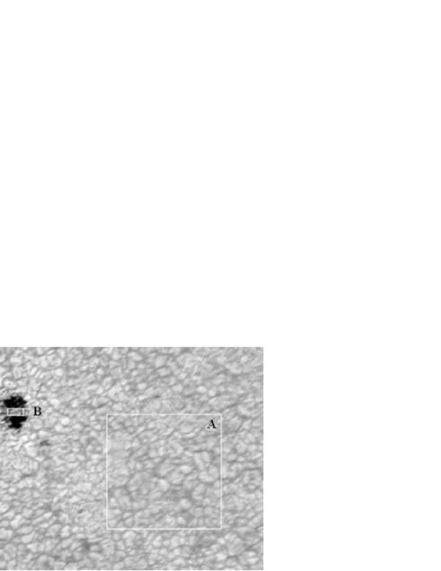
Figure 1: Broad-band image of the FoV, including the pore, after applying a speckle restoring program. We outline the analyzed regions: the quiet granular field ($A$) and the light bridge ($B$).

The observations were performed on September, 28th 2005 at the 0.76 m DST in Sunspot, New Mexico. We observed a central region of the solar disk including a pore with light bridge (AR10812). The interferometer used for these observations was the Interferometric BI-dimensional Spectrometer (IBIS) (Cavallini, 2006), fed by the High Order Adaptive Optics (HOAO) system (Rimmele, 2004) tracking the pore.
The IBIS instrument allows us to obtain solar monochromatic images with high spatial ($\simeq$ 0.2 arcsec), spectral ($\lambda/\Delta\lambda=2\cdot 10^{5}$) and temporal resolution (exposure time $\simeq 10\leavevmode\nobreak\ ms$; acquisition rate $\simeq 5$ frames$\cdot$ $s^{-1}$). IBIS essentially is formed by two air-spaced Fabry Perot Interferometers (FPIs), 50 mm in diameter, used in classical mount and in axial mode, in series with one of five prefilters with FWHM of 0.3 nm to 0.5 nm, depending on wavelength, mounted on a filterwheel. Monochromatic images, consisting of 80” diameter circular section, are recorded by a Princeton CCD camera. The detector is a Kodak KAF-1400 with 1317 $\times$ 1035 pixels, a dynamic range of 12 bits and an acquisition rate of 5 Mpixels$\cdot s^{-1}$. IBIS is equipped with a white light channel, that provides broad-band images with a 5.0 nm passband around 700.0 nm, strictly simultaneous to the narrow-band ones.
The dataset used in this paper consists of 200 sequences, containing a 16 image scan of the Fe I 709.0 nm line, a 14 image scan of the Fe II 722.4 nm line and 6 spectral images of the Ca II 854.2 nm line (one line core image and 5 line wing images). The exposure time for each monochromatic image was 25 ms. The CCD camera was rebinned to 512 $\times 512$ pixels, so that the final pixel scale for the images was $0.17"\cdot$pixel^-1. The time interval between two successive images and two successive spectral series was 0.3 s and 14 s, respectively.
In addition to the narrow-band images, G-band images were simultaneously recorded.

2.2 Standard reduction of IBIS data

The first step in the data reduction is to correct both the data and the flatfield images for dark current and CCD non-linearity effects. Regarding the flatfield correction, we have to consider the blueshift effect due to the classical mounting of the two FPIs. In this configuration every image point corresponds to rays with a specific angle with respect to the optical axis propagating through the FPIs. This causes a systematic blueshift of the instrumental profile when moving from the optical axis towards the edge of the FoV, therefore reaching its maximum in the outermost pixels. This maximum is about 0.6 nm at 600.0 nm wavelength and is about 1.0 nm at 850.0 nm wavelength.
To produce the gain table, we compute a “flatfield scan” averaging the 100 flatfield sequences for each spectral point. We then determine the instrumental blueshift map by calculating the line core shifts of all the pixels in the FoV with respect to the reference profile and fitting this resulting map with a parabolic surface.

The reference profile is obtained by averaging the line profiles of the pixels in a central region (100 $\times$ 100 pixels) of the FoV. In order to obtain an average spectral profile, all pixel profiles are remapped to a common wavelength scale by applying the blueshift map and then averaged. The remapping process is performed by linearly interpolating the measured spectral profiles. The average spectral profile is then applied on each pixel and shifted accordingly to the blueshift map in order to construct the ideal blueshifted flat field scan that is expected for a “perfect” system (i.e. with only the blueshift contribute and no gain variation). Any differences between the flat field scan and the ideal blueshifted flat field scan are due to spatial inhomogeneities in the system response. The final gain table scan is constructed by dividing the flat field scan by the ideal blueshifted flat field scan, so that it does not contain unwanted spectral information. The gain table is then applied to the raw data in order to correct each pixel for the flat field response. Finally, the blueshift correction for the flat fielded data is computed and applied with the same process used for the flat fields.

2.3 Key properties of IBIS photospheric and chromospheric lines

To associate to observed photospheric lines a suitable “formation zone”, we study their sensitivity, as a function of the depth, to the perturbations of velocity. In detail, we treat the effects of linear dynamic perturbations on the line profiles and study the velocity response functions $RF_{\,V}$ of the emergent intensity at the observed wavelengths within the lines (Caccin et al., 1977; Berrilli et al., 2002), that provide the corresponding intensity perturbation as:

$$\delta I(\lambda)=\int_{-\infty}^{+\infty}v(z)RF_{V}(z,\lambda)dz.$$ (1)

The velocity response function is computed by using the usual formula:

$$RF_{V}(z,\lambda)=\frac{\partial\chi(z,\lambda,v)}{\partial v}(S(z,\lambda)-I(z,\lambda))e^{-\tau(z,\lambda)}.$$ (2)

where $\chi(z,\lambda,v)$ is the total opacity for volume unit, $S(z,\lambda)$ the source function and $\tau(z,\lambda)$ the optical depth.

$$\begin{array}[]{l l c c r c}\hline\cr\vskip 3.0pt plus 1.0pt minus 1.0pt\cr$$Line&\chi_{ion}\,(eV)&\chi_{ex}\,(eV)&\lg(gf)&\zeta&\xi\,(km/s)$$\\ \vskip 3.0pt plus 1.0pt minus 1.0pt\cr\hline\cr\vskip 3.0pt plus 1.0pt minus 1.0pt\cr$$FeI\phantom{1}\,709.0\,\phantom{1}nm&\phantom{1}7.87&4.231&-1.3&17&1.00$$\\ $$FeII\,722.4\,\phantom{1}nm&16.18&3.889&-3.3&50&1.75$$\\ \vskip 3.0pt plus 1.0pt minus 1.0pt\cr\hline\cr\end{array}$$

Table 1: Line parameters used for the calculation of line profiles. $\zeta$ is a fudge factor multiplying the Unsöld value of $\gamma$ in the Lorentz part of the absorption profile, while $\xi$ is the usual microturbulence term. The values of $\zeta$ and $\xi$ are chosen to optimize the comparison with atlas data.

For the calculation we adopted LTE approximation, so that the $S(z,\lambda)$ is velocity independent, and we use Kurucz’s solar atmospheric model (Kurucz, 1994). The validity of this model and of the line parameters we used (Table 1) is given by the comparison between the theoretical synthesis of the lines and the atlas data (Kurucz et al., 1985).
The formation depth, i.e. the location of the maximum of the $RF_{V}$, depends on the wavelength, hence on the given points of the line profile. This dependence is more evident for the Fe I 709.0 nm line (Fig. 2), while for Fe II 722.4 nm the $RF_{V}$ maximum is almost the same for each wavelength (Fig. 3). Since we derive the velocity shift by a fitting procedure that uses all the sperimental spectral points, we consider the mean of the corresponding $RF_{V}$. The formation heights for the average lines are reported in Table 2.
The Ca II 854.2 nm chromospheric line forms at $\simeq 800$ km above the photosphere. Our observations, on the red wing of this line ($\lambda_{0}$ + 12 nm), may be associated to a photospheric height, as indicated by the Contribution Functions computed for a quiet Sun model (Qu & Xu, 2002). This estimation is an approximation as the region we observe is deeply immersed in a non-quiet and non-homogeneous atmosphere.

$$\begin{array}[]{l l l l}\hline\cr\vskip 3.0pt plus 1.0pt minus 1.0pt\cr$$Line&h_{core}\,\,(km)&h_{mean}\,\,(km)&FWHM$$\\ \vskip 3.0pt plus 1.0pt minus 1.0pt\cr\hline\cr\vskip 3.0pt plus 1.0pt minus 1.0pt\cr$$FeI\phantom{1}\,709.0\phantom{1}nm&150&100&200$$\\ $$FeII\,722.4\phantom{1}nm&\phantom{1}40&\phantom{1}40&140$$\\ \hline\cr\end{array}$$

Table 2: Line formation depth for the line center and the whole line. The latter is obtained by averaging the different $RF_{V}$ computed in the sperimental wavelenghts and its FWHM is also given.

Figure 2: Velocity response function for the Fe I 709.0 nm line. $Solid$ $line$: average $RF_{V}$; $Dotted$ $line$: center line position $\lambda_{0}$.

Figure 3: Velocity response function for the Fe II 722.4 nm line. $Solid$ $line$: average $RF_{V}$; $Dotted$ $line$: center line position $\lambda_{0}$.

2.4 LOS Velocity maps

Vertical velocity maps were computed for the Fe I 709.0 nm and Fe II 722.4 nm lines by applying a line-profile Gaussian fit to the monochromatic cube of images and then transforming Doppler shifts in LoS velocities. The same procedure has been used to compute spectral line core intensity and FWHM maps.
In order to study the convection dynamics, before analyzing velocity and intensity fields, we have to take into account the 5-min acoustic oscillations. These are removed by applying a $k_{h}-\omega$ subsonic filter: we cut a cone out of the $k_{h}-\omega$ space whose outer borders correspond to $7\leavevmode\nobreak\ km\leavevmode\nobreak\ \cdot s^{-1}$.
After the application of the subsonic $k_{h}-\omega$ filter on the time series of continuum, velocity and center-line intensity maps, we consider a region of interest (Fig. 1) centred on the pore of about 27”$\times$27”.
This is the region tracked by the adaptive optic system, so we are confident that it is characterized by a high spatial resolution.
In our analysis, we neglect the velocity offset due to the convective blueshift (Keil et al., 1999) and define absolute values by setting to zero the mean velocity of the whole observed field.

3 Results and discussion

In order to study the evolution of AR10812, we examined high resolution MDI continuum images, corresponding to three days before our observation run, and established that it was made up of two different structures, showing the same polarity. If we look at AR10812 three days after our observation date, we see that the photospheric and magnetic signatures have disappeared.

3.1 Radial structure of the pore

Figure 4: Upper panel: plot of the mean radial LOS velocity inside the pore; lower panel: plot of the mean radial intensity (solid) and of its derivative (dotted).

We investigated the radial structure of the circular pore, by computing the azimuthal average LoS velocity and intensity excluding the light bridge contribution. We focus our analysis on the Fe I 709.0 nm LoS velocity maps. By analyzing the plot shown in the upper panel of Fig. 4 it is worth noting that an annular downflow lies just outside the pore border, as identified by the maximum in the derivative of the intensity. From a qualitative point of view the LoS velocity shows three different behaviors: it results negative and quasi-constant inside the umbra; it reaches its largest negative values, $\sim-500m\cdot s^{-1}$, just outside the umbra; beyond this downflow region the velocity increases toward typical granular values.
A more careful investigation of the annular downflow region points out an irregular form in space and an intermittent behavior in time. As a matter of fact, a time-slice representation (Fig. 5, $right$ $panel$) of this downflow region shows that recurrent strong downflows are present in the upper-left boundary of the pore, this resulting in persistent downflows in the whole period averaged LoS velocity map (Fig. 5, $left$ $panel$).

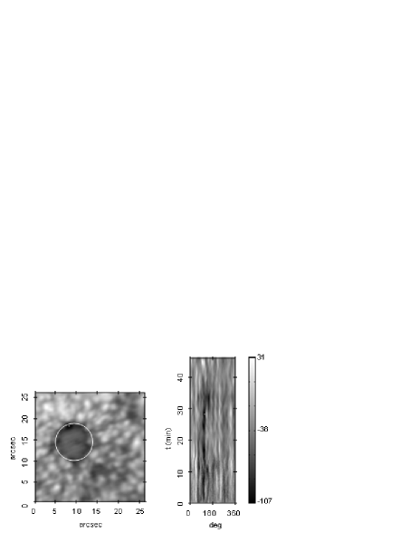
Figure 5: $Left$ $panel$: time averaged Doppler map of the analyzed pore region; $right$ $panel$: time-slice of the circular ring (white circle) surrounding the umbra. It is obtained by following the evolution of the structures covered by the circle surrounding the pore. The center of our polar coordinates system corresponds to the center of the pore.

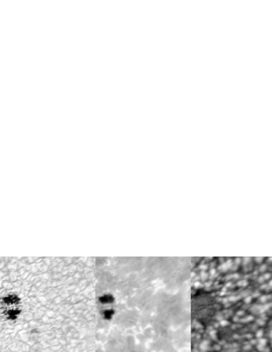
Figure 6: The (AR10812) pore region intensity, as observed with the broad-band channel of IBIS (left panel) and on the red wing of Ca II 854.2 nm line (central panel). The corresponding LoS velocity pattern, computed from Doppler shifts of Fe I 709.0 nm line, is shown in the right panel, a bright (upward) LoS velocity feature is clear visible along the light bridge axis. The white segments orthogonal to the light bridge, drawn in the left panel figure, denote the cuts across which the intensity and velocity profiles plotted in Fig. 7 have been computed.

3.2 Intensity and velocity structure inside the pore

The dynamics of the light bridge are investigated by means of intensity and LoS velocity maps. Fig. 6 shows the pore region intensity, as observed with the broad-band channel of IBIS and on the red wing of CaII 854.2 nm line, and the corresponding LoS velocity pattern, computed from Doppler shifts of Fe I 709.0 nm line. The intensity and velocity profiles, along slices which are orthogonal to the light bridge, are shown in Fig. 7.
From our analysis we may distinguish two major outcomes: the presence of elongated features, both in intensity and in LoS velocity images, and the occurrence of a kind of reversing in intensity and velocity of small scale features, i.e. intensity maxima along the light bridge match more intense downward velocities.
The observed reversing in the LB intensity and velocity frames, recalls the inverse granulation phenomenon, which consists of the inversion of temperature fluctuations, with respect to velocity field, in the upper photosphere. The occurrence of reversed granulation, around 120 km above quiet Sun photosphere, was observed at disk center in Fe I 537.9 nm and Fe I 557.6 nm photospheric lines by THEMIS in IPM imaging mode (Berrilli et al., 2002). Successively, Puschmann et al. (2003) reported an inversion of temperature, at a height of $\simeq 140\leavevmode\nobreak\ km$, using one-dimensional slit-spectrograms taken in quiet sun. More recently, Janssen & Cauzzi (2006) confirmed that reversed granulation is also visible at $\simeq 200\leavevmode\nobreak\ km$ using FeI 709.0 nm line center images. However, the inverse granulation phenomenon involves the upper quiet photosphere, whereas dark intensity features in broad-band channel images refer to a zero altitude photosphere. Moreover, our observations show that an elongate structure along the axis of the light bridge exists also in velocity maps. More in detail, our highest resolution images show that a weak upflow, $\sim 50\div 100\leavevmode\nobreak\ m\cdot s^{-1}$, is present along the light bridge axis, while a downflow, $\sim-(200\div 300)\leavevmode\nobreak\ m\cdot s^{-1}$, exists along the boundary. The topology of such a velocity structure resembles some roll features known from laboratory experiments on Rayleigh-B$\acute{e}$nard convection and may be a signature of modified photospheric convective flows confined by two magnetic walls.

3.3 A light bridge dark lane semi-analytical model

The presence of a narrow central dark lane running along the axis of the light bridges is a common feature of LBs. Its existence is reported in Sobotka et al. (1994) and with more details in (Berger & Bierdyugyna, 2003; Lites et al., 2004). Evidence of a magnetoconvective origin for a sunspot light bridge is reported by Rimmele (1997). Recently, Spruit & Scharmer (2006) argued that a 3D radiative magnetohydrodynamic Nordlund & Stein simulation may explain the formation of a dark lane inside the light bridge as a consequence of the higher gas pressure in the field-free part of the photosphere, trapped between two magnetic fields.
To reproduce this configuration, we developed a simple thermal model of the light bridge, in which we consider a quiet, field free model below a magnetic zone partially emptied of plasma (see Fig. 8).
The thermal quantities, relative to the quiet sun (field-free), are given by the following analytic expressions, that well fit the solar Kurucz model (Kurucz, 1994):

$$\rho_{q}(\zeta) = \rho_{q}\frac{e^{z/H}}{e^{z/H}+1}=\rho_{0}\frac{\zeta-1}{\zeta}$$

$$P_{q}(\zeta) = P_{q}ln(\zeta)$$

$$T_{q}(\zeta) = T_{q}\frac{\zeta}{\zeta-1}ln(\zeta)$$

where $\zeta=e^{z/H}+1$ and z is the depth. This model satisfies the hydrostatic equation ($P_{q}=g\rho_{q}H$) and the perfect gas law ($T_{q}=\mu P_{q}/R\rho_{q}$). The two parameters H and $\rho_{q}$ are fixed so as to optimize the comparison with the Kurucz model ($\rho_{q}=5.007\cdot 10^{-7}\leavevmode\nobreak\ gr\cdot cm^{-3}$ and $H=100\leavevmode\nobreak\ km$).
For the magnetic atmosphere, we mimic the presence of the magnetic field through a model with an exponential density law:

$$\rho_{b}(\zeta) = \rho_{b}(\zeta-1)^{\alpha}$$

$$P_{b}(\zeta) = P_{b}(\zeta-1)^{\alpha}$$

$$T_{b}(\zeta) = T_{b}$$

where $\alpha$ is the ratio between the scale height of quiet and magnetised model ($\alpha=H/H_{b}$, $P_{b}=g\rho_{b}H_{b}$ and $T_{b}=\mu/RgH_{b}$). In order to calculate the emergent intensity we need an expression for the opacity. We use the usual formula: $k(P,T)\propto P^{A}T^{B}$, where $A=0.5$ and $B=8$. These values are obtained through the best fit of the opacity tables computed by Kurucz (1994). The $H_{b}$ parameter is a free parameter set to 120 km in order to match the observed contrast ($\simeq 1.5$) between umbra and quiet granular field. Eventually, the model (Fig. 8) uses two atmospheres (field-free and magnetic) to create a simplified geometry above the light bridge. The geometry of the separating surface is described by two functions: a linear function ($z_{t}=a\cdot x$) and a cubic function ($z_{t}=b\cdot x^{3}$), where x is the horizontal coordinate. We adopt a quiet model for $z>z_{t}$ and a magnetic model for $z<z_{t}$. Considering the observations, we fix the light bridge width to 1500 km. In Fig. 9 we show the intensity profile inside the light bridge for the two adopted geometries. It’s worth to note that both geometries are able to qualitatively reproduce the presence of a dark lane across the light bridge, but with the cubic function we obtain a contrast profile, that better matches the observed one.

Figure 7: Plots of the light bridge intensity, in the broad-band channel of IBIS (upper panel) and in the red wing of the Ca II 854.2 nm line (central panel) and of the corresponding Fe I 709.0 nm line LoS velocity (lower panel). All profiles have been computed along the segments shown in Fig. 6 and have been shifted vertically by arbitrary amounts to provide separation.

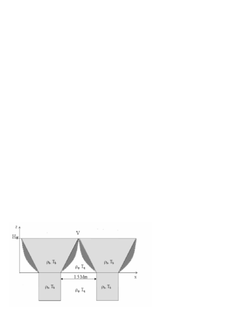
Figure 8: Cross-section of the light bridge structure modeled as a field free plasma (white region) trapped by two magnetic flux tubes (grey regions). Two different geometries are considered for the surfaces separating the quiet and magnetic atmospheres: a straight line (bold) or a cubic function (dotted).

Figure 9: Synthetic emergent intensities across the light bridge for the two different geometries of the separating surface: a straight line (upper panel) or a cubic function (lower panel). In both figures the three plots correspond to different $H_{ff}$ values (where $H_{ff}$ is the height of the V point shown in Fig 8): 200 km, 300 km and 400 km for solid, dotted and dashed lines, respectively.

4 Conclusions

A pore with a light bridge (AR10812) was observed at high spatial and spectral resolution. From MDI/SOHO magnetograms and continuum images, we established that the observed region, initially composed of two structures with the same polarity, disappears three days after our observation. Such a topology allows to relate the observed light bridge properties to the contiguity of two flux tubes. With the aim to investigate the photospheric environment of the pore and the nature of the bright structure inside it, we computed the intensity and photospheric LoS velocity maps. In particular, we analyzed the intensity maps provided by the broad-band channel of IBIS and by the red wing of Ca II 854.2 nm line, and the corresponding Fe I 709.0 nm line LoS velocity fields.
Our main conclusions are:

• The pore is characterized by a downward average velocity of $\sim-200\leavevmode\nobreak\ m\cdot s^{-1}$ in the umbra and of $\simeq-350\leavevmode\nobreak\ m\cdot s^{-1}$ in the surrounding annular region. The presence of downflows around magnetic structures has been predicted by numerical models (e.g.Steiner et al. (1998); Hulburt & Rucklidge (2000)) and reported in recent observations (e.g. Keil et al. (1999); Sankarasubramanian & Rimmele (2003)).

• The time-slice of the annular region, irregular in shape and intermittent in time, shows that recurrent strong downflows are present in the boundary of the pore, resulting in persistent downflows in the averaged LoS velocity map.

• An analysis of the intensity and velocity maps and of the relative profiles, calculated along cuts perpendicular to the axis of the light bridge, reveals the presence of elongated structures, showing a kind of reversing in intensity and velocity. More in detail, in intensity images we observe a narrow central dark lane running along the axis of the light bridge. This structure, in our best highest resolution LoS velocity images, matches to a weak upflow, around $50\div 100\leavevmode\nobreak\ m\cdot s^{-1}$, flanked by two downflows, around $-(200\div 300)\leavevmode\nobreak\ m\cdot s^{-1}$. The topology of such a velocity structure resembles a convective roll and may indicate a modification of the photospheric convective flows.

• We present a semi-analytical model for the light bridge, in which we consider a quiet, field free region trapped by two magnetic walls, able to qualitatively reproduce the observed intensity behavior inside the light bridge.

By considering the evolution of the analyzed region and taking into account a simulation by Hulburt & Rucklidge (2000), we model the observed pore (Fig.10) as resulting from the merging of two separate magnetic structures with the same polarity both surrounded by downward flows. These downflow structures persist in the quenching region, where the convection results strongly modified by the presence of the magnetic field, and in the annular region surrounding the pore.
This interpretation is supported by the observed time averaged LoS velocity structure reported in Fig.7. This LoS velocity profile is calculated along a cut orthogonal to the light bridge and crosswise to the pore. Our scheme is analogous to that reported by Jurĉ$\acute{a}$k et al. (2006) to explain the magnetic canopy above light bridges.
As final remark, since bright features inside pores and sunspots show a large zoology, it should be clear that further work is needed on this subject, including a deep investigation of how the magnetic field modifies the local photosphere and chromosphere.

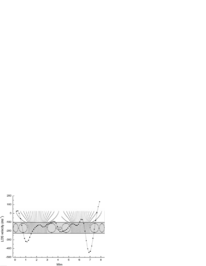
Figure 10: Schematic cross-section of the analyzed structure. In the background a sketch of the flows around the pore: the model is obtained by considering two magnetic flux tubes, each derived from the simulation by Hulburt et al. Hulburt & Rucklidge (2000). Superimposed is the computed mean LoS velocity, averaged along the pore (dot+spline).