Role of interference in quantum state transfer through spin chains

Abstract

We examine the role that interference plays in quantum state transfer through several types of finite spin chains, including chains with isotropic Heisenberg interaction between nearest neighbors, chains with reduced coupling constants to the spins at the end of the chain, and chains with anisotropic coupling constants. We evaluate quantitatively both the interference corresponding to the propagation of the entire chain, and the interference in the effective propagation of the first and last spins only, treating the rest of the chain as black box. We show that perfect quantum state transfer is possible without quantum interference, and provide evidence that the spin chains examined realize interference-free quantum state transfer to a good approximation.

I Introduction

Recently, the idea to use quantum spin chains for short-distance quantum communication was put forward by Bose Bose (2003). He showed that an array of spins (or spin-like two level systems) with isotropic Heisenberg interaction is suitable for quantum state transfer. In particular, spin chains can be used as transmission lines for quantum states without the need to have controllable coupling constants between the qubits or complicated gating schemes to achieve high transfer fidelity. Alice prepares an input state on the first spin of the chain at time $t=0$ (all other spins are in the state down/zero), and after a certain time $t_{1}$ Bob recovers an output state on the last spin at the other end, while Alice normally looses her state, in fulfillment of the no-cloning theorem Wootters and Zurek (1982). Bose showed that the average fidelity of the quantum state transfer exceeds the maximum value which can be achieved classically for spin chains of length $N$ up to $N\sim 80$. The method was later extended using engineered coupling constants Christandl et al. (2004); Yung et al. (2004); Lyakhov et al. (2005), multi-spin encoding Osborne and Linden (2004), as well as “dual-rail encoding” in two parallel quantum channels Burgarth and Bose (2005a, b). In Wójcik et al. (2005) it was shown that the transmission even through very long chains can be improved to almost perfect fidelity if the coupling of the first and last spins to the chain is reduced.

As with any task in quantum information processing which offers an advantage over classical information processing, the question arises what in the quantum world allows for that advantage. It is generally acknowledged that quantum entanglement and interference are two ingredients which distinguish quantum information processing from its classical counterpart Bennett and DiVincenzo (2000). Quantum entanglement has been studied in great detail over the last fifteen years Lewenstein et al. (2000), but the precise role of interference in various quantum information treatment tasks remains to be elucidated Beaudry et al. (2005).

Contrary to entanglement, interference is a property not of a quantum state but of the propagator of a state. This is due to the fact that the coherence of the propagation is important for interference. Indeed, the final probability distribution resulting from a given quantum algorithm can always be generated through stochastic simulation on a classical computer as well: for a known quantum circuit and initial state one can in principal calculate the final state, and therefore the probability distribution. It is then simple to create a stochastic process which gives each possible outcome with the correct probability. In such a classical simulation clearly no interference takes place. Thus, what counts for interference is not a state itself but the way it was created.

A quantitative measure of interference in any quantum mechanical process in a finite-dimensional Hilbert space was recently introduced in Braun and Georgeot (2006), and the statistics of quantum interference in random quantum algorithms was studied in Arnaud and Braun . Here we propose to study the role of interference in quantum state transfer through spin chains. After defining the notion of interference, reduced interference, and fidelity in Section II, we will follow two complementary approaches: in Section III we will consider the spin chain as a black box which propagates the initial state of the first and last spins combined to a final state of these two spins. We will calculate the reduced interference that describes this propagation for different spin chains and show that perfect state transfer is possible without quantum interference. In Section IV we will then consider the unitary evolution of the entire chain and analyze this unexpected result.

II Interference and reduced interference

The interference $I(t)$ for a general quantum process described by a propagator $\mathcal{P}(t)=P_{ij,kl}(t)$ which propagates an initial state $\rho$ with matrix elements $\rho_{ij}$ in a fixed orthonormal basis of dimension $D$ to a final state $\rho^{\prime}$,

$$\rho^{\prime}_{ij}=\sum_{k,l=1}^{D}P_{ij,kl}\rho_{kl}$$ (1)

is defined as Braun and Georgeot (2006)

$$I(t)=\sum_{i,k,l}|P_{ii,kl}(t)|^{2}-\sum_{i,k}|P_{ii,kk}(t)|^{2}\,.$$ (2)

If $\mathcal{P}$ describes the propagation of the reduced density matrix of the first and last spins alone (which will be mixed in general, as it results from tracing out the intermediate spins of the chain), Eq. (2) defines the “reduced interference” $I_{r}(t)$. We will evaluate $I_{r}(t)$ analytically for spin chains which conserve the number of excitations in the chain, and show that $I_{r}(t)$ is intimately linked to the average fidelity $F(t)$ introduced in Bose (2003),

$$F(t)=\frac{1}{4\pi}\int\langle\psi_{in}|\rho_{out}(t)|\psi_{in}\rangle d\Omega\,,$$ (3)

where $|\psi_{in}\rangle$ is the pure state to be transmitted prepared on the first spin, $\rho_{out}$ is the output state on the last spin (i.e. $\rho_{out}=\mathrm{Tr}_{1}\rho^{\prime}$, with the trace over the first (input) spin), and the integral is over all initial states of the input spin on the Bloch sphere parameterized by the spatial angle $\Omega$. $F(t)$ is a function of time and we are interested in the maximum fidelity in some reasonable time interval, that is less than the decoherence time of the qubits, and scales like the inverse coupling Bose (2003). We will also provide numerical results for $I_{r}(t)$ for chains in which the number of excitations is not conserved.

The interference measure for the unitary propagation of the entire chain, $|\psi^{\prime}\rangle=U|\psi\rangle$ reduces to Braun and Georgeot (2006)

$$I_{U}(t)=D-\sum_{i,k=1}^{D}|U_{i,k}(t)|^{4}\,.$$ (4)

For this coherent propagation, the interference $I_{U}(t)$ measures the degree of equipartition of the output that result from any basis state of a system at $t=0$. Here, an equipartitioned state means a state that is a superposition of all the basis states with amplitudes of modulus $1/\sqrt{D}$. For better comparison of the results we will plot the normalized interference $I=I_{U}/(D-1)$ so that the maximal possible value of the interference is one and does not depend on the number of qubits in the chain.

III Reduced interference for excitation-conserving spin chains

We start by evaluating the reduced interference in excitation-preserving chains, i.e., spin chains for which the total Hamiltonian $H$ commutes with the total spin component $S^{z}=\sum_{i=1}^{N}\sigma_{i}^{z}$. The particular example of the chain with isotropic Heisenberg interaction proposed by Bose Bose (2003) falls into this class (see Section III.1 below). We start with at most one excitation in the chain and limit ourselves to pure initial states. Therefore one can specify a state of the entire chain $|j\rangle$ ($j=1,\ldots,N$) by the position at which the excitation is localized. In principle there are four computational basis states for the two spins, but the state where both the first and the last spins are excited will never appear. We therefore restrict our attention to the three-dimensional Hilbert space spanned by the states $|1\rangle$, $|N\rangle$, and $|0\rangle_{r}$ (the state where both the first and the last spins are not excited). We will also make use of the state $|0\rangle_{m}$ of the intermediate part of the chain, where all intermediate spins are not excited.

We start from an initial state of the chain which factorizes between the two selected spins ($1$ and $N$) and the rest of the chain, which is assumed to be in state $|0\rangle_{m}$,

$$|\Psi_{in}\rangle=(a_{0}|0\rangle_{r}+a_{1}|1\rangle+a_{N}|N\rangle)|0\rangle_{m}\,.$$ (5)

The initial reduced density matrix of the first and last spins,

$$\rho=\left(\begin{array}[]{ccc}|a_{0}|^{2}&a_{0}a_{1}^{*}&a_{0}a_{N}^{*}\\ a_{1}a_{0}^{*}&|a_{1}|^{2}&a_{1}a_{N}^{*}\\ a_{N}a_{0}^{*}&a_{N}a_{1}^{*}&|a_{N}|^{2}\end{array}\right)\,,$$ (6)

then still represents a pure state. For any Hamiltonian that conserves the number of excitations we can write the state at time $t$ as

$$|\Psi_{out}(t)\rangle=a_{0}|0\rangle_{r}|0\rangle_{m}+a_{1}\sum_{j=1}^{N}\langle j|e^{-iHt}|1\rangle|j\rangle+a_{N}\sum_{j=1}^{N}\langle j|e^{-iHt}|N\rangle|j\rangle\,,$$ (7)

or

$$|\Psi_{out}(t)\rangle=a_{0}|0\rangle_{r}|0\rangle_{m}+a_{1}f_{11}|1\rangle|0\rangle_{m}+a_{1}\sum_{j=2}^{N-1}\langle j|e^{-iHt}|1\rangle|0\rangle_{r}|j\rangle+a_{1}f_{N1}|N\rangle|0\rangle_{m}+$$

$$a_{N}f_{1N}|1\rangle|0\rangle_{m}+a_{N}\sum_{j=2}^{N-1}\langle j|e^{-iHt}|N\rangle|0\rangle_{r}|j\rangle+a_{N}f_{NN}|N\rangle|0\rangle_{m}\,,$$ (8)

where

$$f_{ij}(t)=\langle i|e^{-iHt}|j\rangle\,.$$ (9)

After tracing out the intermediate spins we obtain the final density matrix of the first and last spins,

$$\rho^{\prime}=\left(\begin{array}[]{ccc}|a_{0}|^{2}+S_{m}&a_{0}(a_{1}^{*}f_{N1}^{*}+a_{N}^{*}f_{NN}^{*})&a_{0}(a_{1}^{*}f_{11}^{*}+a_{N}^{*}f_{1N}^{*})\\ a_{0}^{*}(a_{1}f_{N1}+a_{N}f_{NN})&|a_{1}f_{N1}+a_{N}f_{NN}|^{2}&(a_{1}f_{N1}+a_{N}f_{NN})(a_{1}^{*}f_{11}^{*}+a_{N}^{*}f_{1N}^{*})\\ a_{0}^{*}(a_{1}f_{11}+a_{N}f_{1N})&(a_{1}f_{11}+a_{N}f_{1N})(a_{1}^{*}f_{N1}^{*}+a_{N}^{*}f_{NN}^{*})&|a_{1}f_{NN}+a_{N}f_{1N}|^{2}\end{array}\right)$$ (10)

where

$$S_{m}=\sum_{j=2}^{N-1}|a_{1}\langle j|e^{-iHt}|1\rangle+a_{N}\langle j|e^{-iHt}|N\rangle|^{2}\,.$$ (11)

Comparing Eqs. (6), (10), and (1) we read off the propagator

$$\mathcal{P}=\left(\begin{array}[]{ccccccccc}1&0&0&0&\sum_{j}|f_{j1}|^{2}&\sum_{j}f_{j1}f_{jN}^{*}&0&\sum_{j}f_{jN}f_{j1}^{*}&\sum_{j}|f_{jN}|^{2}\\ 0&f_{N1}^{*}&f_{NN}^{*}&0&0&0&0&0&0\\ 0&f_{11}^{*}&f_{1N}^{*}&0&0&0&0&0&0\\ 0&0&0&f_{N1}&0&0&f_{NN}&0&0\\ 0&0&0&0&|f_{N1}|^{2}&f_{N1}f_{NN}^{*}&0&f_{NN}f_{N1}^{*}&|f_{NN}|^{2}\\ 0&0&0&0&f_{N1}f_{11}^{*}&f_{N1}f_{1N}^{*}&0&f_{NN}f_{11}^{*}&f_{NN}f_{1N}^{*}\\ 0&0&0&f_{11}&0&0&f_{1N}&0&0\\ 0&0&0&0&f_{11}f_{N1}^{*}&f_{11}f_{NN}^{*}&0&f_{1N}f_{N1}^{*}&f_{1N}f_{NN}^{*}\\ 0&0&0&0&|f_{11}|^{2}&f_{11}f_{1N}^{*}&0&f_{1N}f_{11}^{*}&|f_{1N}|^{2}\\ \end{array}\right)\,,$$ (12)

where the rows and columns are in the order $00$, $01$, $0N$, $10$, $11$, $1N$, $N0$, $N1$, $NN$.

Inserting $\mathcal{P}$ into Eq. (2), we obtain

$$I_{r}(t)=\left|\sum_{j=2}^{N-1}\langle j|e^{-iHt}|1\rangle\langle N|e^{iHt}|j\rangle\right|^{2}+\left|\sum_{j=2}^{N-1}\langle j|e^{-iHt}|N\rangle\langle 1|e^{iHt}|j\rangle\right|^{2}$$

$$+|f_{N1}f_{NN}^{*}|^{2}+|f_{NN}f_{N1}^{*}|^{2}+|f_{11}f_{1N}^{*}|^{2}+|f_{1N}f_{11}^{*}|^{2}$$ (13)

for the reduced interference. This expression can be further simplified by using

$$\sum_{j=1}^{N}\langle N|e^{iHt}|j\rangle\langle j|e^{-iHt}|1\rangle=\langle N|1\rangle=0\,,$$ (14)

such that

$$I_{r}(t)=2\left|f_{11}f_{N1}^{*}+f_{N1}f_{11}^{*}\right|^{2}+2|f_{11}f_{1N}^{*}|^{2}+2|f_{N1}f_{NN}^{*}|^{2}\,.$$ (15)

This result is valid for any Hamiltonian of the entire chain that conserves the number of excitations. In the case of a linear chain with symmetrical nearest-neighbor interactions (i.e. the Hamiltonian is invariant under relabeling the qubits $1,2,..,N$ into $N,...,2,1$), we have $f_{1N}=f_{N1}$ and $f_{11}=f_{NN}$. The reduced interference can then be expressed using two amplitudes of the state transfer,

$$I_{r}(t) = 8|f_{11}|^{2}|f_{1N}|^{2}+2f_{11}^{2}(f_{1N}^{*})^{2}+2f_{N1}^{2}(f_{11}^{*})^{2}$$ (16)

$$= 4|f_{11}|^{2}|f_{1N}|^{2}(1+2\cos^{2}(\gamma_{11}-\gamma_{1N}))\,,$$

where $\gamma_{ij}=\arg(f_{ij})$. We are now in the position to evaluate $I(t)$ for specific examples.

III.1 Chains that conserve the number of excitations

Let us first consider the spin chains studied in Bose (2003). They consist of a one-dimensional array of $N$ spins, with nearest-neighbor spins coupled through an isotropic Heisenberg interaction. The Hamiltonian of the chain reads

$$H=-\sum_{i=2}^{N}J\bm{\sigma}_{i}\cdot\bm{\sigma}_{i-1}-\sum_{i=1}^{N}B_{i}\sigma_{i}^{z}\,,$$ (17)

where $\bm{\sigma}_{i}=(\sigma_{i}^{x},\sigma_{i}^{y},\sigma_{i}^{z})$ denotes the vector of the Pauli matrices on site $i$, $B_{i}$ denotes the site-dependent static magnetic field and $J>0$ is the coupling strength, taken as constant for all spins.

Bose showed that the average fidelity, Eq. (3), for this model is given by

$$F=\frac{|f_{1N}|\cos\gamma_{1N}}{3}+\frac{|f_{1N}|^{2}}{6}+\frac{1}{2}\,.$$ (18)

At $t=0$, $f_{1N}=0$ for $N>1$, such that the average fidelity corresponds to the fidelity of a random guess of Bob of the quantum state of Alice ($F=1/2$). The overlap $f_{1N}(t)$ becomes appreciable, once the spin wave excited at Alice’s end arrives at Bob’s spin. Perfect state transfer for all states ($F=1$) requires $f_{1N}=1$, along with $\cos\gamma_{1N}=1$. The last equality can always be achieved by varying the magnetic fields $B_{i}$. From here on we will assume that this is the case and therefore put $f_{1N}=|f_{1N}|$ when plotting fidelities of the state transfer.

By comparing Eqs. (16) and (18) one can see that interference is determined by one more complex variable $f_{11}$ compared to the fidelity. Therefore, in general there is no explicit formula that describes interference in terms of fidelity alone. Naively one might expect that interference should play an important role for quantum state transfer, if the fidelity of the process exceeds the maximal classical value, $F=2/3$ Horodecki et al. (1999). However, note that an ideal quantum state transfer can be realized through the permutation of the first and the last spins $|0\rangle_{r}\leftrightarrow|0\rangle_{r}$, $|1\rangle\leftrightarrow|N\rangle$, which does not lead to any interference at all. In general, interference measures both the equipartition of all output states for any computational basis state as input, and the coherence of the propagation. “Coherence” was defined in Braun and Georgeot (2006) as the sensitivity of the final probabilities $\rho^{\prime}_{ii}$ to the initial phases. As is evident from Eq. (1), the only phase information which contributes to the reduced interference in the propagation through the spin chain is the relative phase between the states $|0\rangle_{r}$ and $|N\rangle$. However, the coherence of the propagation becomes irrelevant for perfect transfer, $f_{1N}=1$, as then $f_{NN}=0$ due to the conservation of the number of excitations, and then the final probabilities do not depend on any initial phases anymore. I.e. for ideal state transfer, the dynamics of the chain indeed realizes the above permutation with vanishing interference. This is also evident from Eq. (16) for $f_{11}=f_{NN}=0$. Note, however, that the interference is finite during the propagation of the signal through the chain, as well as quite generally for any situation in which neither $f_{11}$ nor $f_{1N}$ vanish. All one can say is that for $F(t)$ close to 1, i.e. $f_{1N}$ close to 1 and thus $f_{NN}$ close to 0, $I_{r}(t)$ remains quite small.

Figure 1 shows $I_{r}(t)$ that was obtained by numerically propagating $|\Psi(t)\rangle$ for $N=20$ (see Eq. (7)) with the Hamiltonian (17). The results are plotted with time in units of $1/J$. We also assumed that $B_{i}=B$ for all $i$ and therefore the interference does not depend on magnetic field. Indeed, in our model $B$ influences only the phases of $f_{11}$ and $f_{1N}$ through a term $\exp(-2iBt)$ (see, for example Bose (2003)) and according to Eq. (16) the interference depends only on phase differences and not on a global phase. One can see that the interference remains quite small. This is because the probability to find an excitation inside the chain is high and both quantities $|f_{11}|^{2}$ and $|f_{1N}|^{2}$ cannot be big ($\sim 0.5$) at the same time at the time scale that is relevant for quantum state transfer.

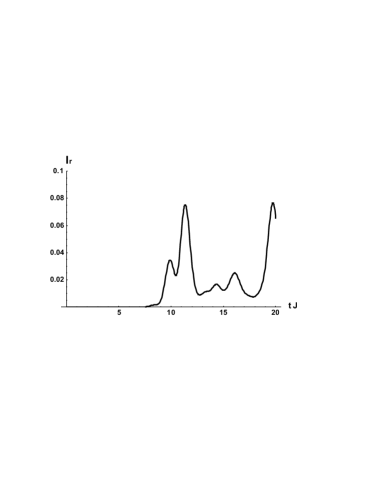
Figure 1: Reduced interference for a spin chain with $N=20$ qubits described by the model defined in Eq. (17).

Let us now consider the case of reduced coupling constants of spins $1$ and $N$ to the rest of the chain

$$H=-\sum_{i=2}^{N}J_{i}(\sigma_{i}^{x}\sigma_{i-1}^{x}+\sigma_{i}^{y}\sigma_{i-1}^{y})\,,$$ (19)

Figure 2: Reduced interference $I_{r}$ for the case of small coupling constants between the first and the last pair of qubits, $N=8$ (blue, thick solid). The green (thin solid) line shows the full interference of the entire chain (renormalized by a factor $1/N$). The black (dot-dashed) line shows the fidelity $F(t)$. The red (dashed) lines are the probabilities to find an excitation on the first qubit and on the last qubit ($|f_{11}|^{2}$ and $|f_{1N}|^{2}$, respectively) if we start with the excitation on the first qubit.

with $J_{2}=J_{N}=aJ$ where $a\ll 1$, and $J_{i\neq 2,N}=J$. It was shown in Wójcik et al. (2005) that this can drastically increase the fidelity of the state transfer. Figure 2 shows the reduced interference $I_{r}(t)$ together with $F(t)$. We see that both are perfectly anticorrelated. In particular, we have again $I_{r}(t)\simeq 0$ for $F(t)\simeq 1$ for the same reasons as discussed before. The interference is maximal half way through the perfect state transfer. In this case, the interference is not small (compare Fig. 1 and Fig. 2) since due to the weak coupling the intermediate spins are only slightly excited Wójcik et al. (2005) and both quantities $f_{11}$ and $f_{1N}$ can be big ($1/\sqrt{2}$) at the same time (see red (dashed) curves in the Fig. 2).

III.2 Chains that do not conserve the number of excitations

Now we consider a more general Hamiltonian that does not conserve the number of excitations,

$$H = -\sum_{i=2}^{N}[J_{xy}(\sigma_{i}^{x}\sigma_{i-1}^{x}+\sigma_{i}^{y}\sigma_{i-1}^{y})+J_{z}\sigma_{i}^{z}\sigma_{i-1}^{z}]$$ (20)

$$- \sum_{i=1}^{N}(\Delta\sigma_{i}^{x}+B\sigma_{i}^{z})\,.$$

Equation (20) is a more realistic model than Eq. (17) since in real qubits the $\sigma^{x}$ term, which describes the tunneling between the states $|0\rangle$ and $|1\rangle$, cannot always be neglected. A physical realization of Hamiltonian (20) was proposed in Lyakhov and Bruder (2005). Sometimes the $\sigma^{x}$ term can be suppressed Levitov et al. (2001); Lyakhov and Bruder (2005), but for longer chains even small values of $\Delta$ will influence the dynamics of the chain. In this case, Eq. (16) is not valid anymore, and the question of how much interference is used in the quantum state transfer needs to be reassessed. Since the number of excitations is not conserved, we have to do the calculation in the much larger Hilbert space with dimensionality $2^{N}$ instead of $N+1$. One can numerically evaluate $\rho^{\prime}(t)$ and find $I_{r}(t)$ as a function of time. We used realistic qubit parameters that are typical for flux qubits, see Orlando et al. (1999); Lyakhov and Bruder (2005), namely $J_{xy}=0.08J_{z}$, and $B=0$. The results of the calculations are shown in Figs. 3 and 4.

Figure 3: Global maxima of $f_{1N}=\langle 1|e^{-iHt}|N\rangle$ in the time interval [0,$1/J_{xy}$] as a function of $\Delta$ for the model defined by Eq. (20), $N=3$.

Figure 4: Reduced interference at the global maxima of $f_{1N}=\langle 1|e^{-iHt}|N\rangle$ in the time interval [0,$1/J_{xy}$], see Fig. 3.

Figure 3 shows the global maxima of $f_{1N}=\langle 1|e^{-iHt}|N\rangle$ in the time interval [0,$1/J_{xy}$] as a function of $\Delta$ for a chain with $N=3$ qubits. The quantity $f_{1N}$ decreases with $\Delta$ until the time required for the state to be transferred from the first to the last qubit is approximately equal to $1/\Delta$. This is in agreement with Lyakhov and Bruder (2005). For large $\Delta$, $f_{1N}$ is close to one due to excitations that are created in the chain during this time interval.

Figure 4 shows the reduced interference at the global maxima of $f_{1N}=\langle 1|e^{-iHt}|N\rangle$ in the time interval [0,$1/J_{xy}$]. Once again, interference decreases with increasing $f_{1N}$, and vice versa, but this time as a function of the parameter $\Delta$. For very small $\Delta$, we have nearly perfect state transfer (almost no equipartition and coherence), therefore the interference is small. It increases with $\Delta$, as the creation of excitations enhances the equipartition and sensitivity of the final state to the initial state. For large $\Delta$, when a high value $f_{1N}$ is achieved due to excitations created in the chain, interference is small. For example if the excitation is created on the last qubit, then the amplitude $|f_{1N}|$ will be equal to one. It corresponds to nearly stochastic transfer, since the final probabilities to find the last qubit in the state $|0\rangle$ or $|1\rangle$ are almost independent of the initial state.

IV Interference in the unitary propagation of the entire chain

The result that perfect quantum state transfer is possible (and realized!) without quantum interference is rather counter-intuitive. It is natural to wonder what happens within the chain. Let us therefore open the black box and study the interference in the propagation of the state of the entire chain (called “full interference” $I=I_{U}/(D-1)=I_{U}/N$ in the following, where confusion is possible) for chains which conserve the number of excitations. This corresponds to a unitary propagation, and we will therefore employ Eq. (4) to quantify the interference.

IV.1 Chain with uniform coupling constants

For a simple chain that consists of more than 3 qubits, the fidelity is always less than one (except the case of specially engineered coupling constants). This is due to the fact, that the the input state gets dispersed over the spins at all times $t>0$.

Using the theory described in Lyakhov and Bruder (2005) we calculated the eigenstates and the eigenenergies of a more general version of the Hamiltonian (17),

$$H=-\sum_{i=2}^{N}[J_{xy}(\sigma_{i}^{x}\sigma_{i-1}^{x}+\sigma_{i}^{y}\sigma_{i-1}^{y})+J_{z}\sigma_{i}^{z}\sigma_{i-1}^{z}]-\sum_{i=1}^{N}B\sigma_{i}^{z}\,.$$ (21)

This Hamiltonian also conserves the number of excitations and describes the chains of superconducting qubits, proposed in Lyakhov and Bruder (2005) and Romito et al. (2005). Knowing the eigenvalues and eigenenergies of (21) allows us to find the matrix elements $U_{ik}$ and numerically calculate the full interference as a function of time and of the number of the qubits in the chain, restricting ourselves again to the $(N+1)$-dimensional Hilbert space of the states in Eq. (5). The results of these calculations are shown in Figs. 5, 6 for $J_{z}/J_{xy}=0.05$ Lyakhov and Bruder (2005).

Figure 5: Fidelity (red, dashed) and normalized full interference (green, solid) for $N=2$ and $N=3$ qubits with uniform coupling constants, Eq. (21).

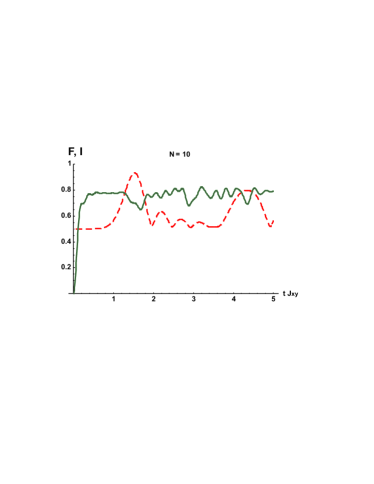
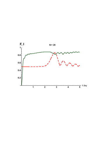
Figure 6: Fidelity (red, dashed) and normalized full interference (green, solid) for $N=10$ and $N=20$ qubits with uniform coupling constants, Eq. (21).

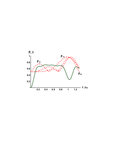
Figure 7: Fidelities (red, dashed) and normalized full interference (green, solid) for $N=6$ qubits with uniform coupling constants, Eq. (21).

Figure 8: Fidelities (red, dashed) and normalized full interference (green, solid) for $N=3$ qubits with uniform coupling constants, Eq. (21).

As we can see in Fig. 5, the full interference is close to zero if the fidelity is close to one. The reason is that the time that is required for the excitation to be transferred from the first to the last qubit (the time of the first fidelity maximum) is approximately equal to the time that it takes for the excitation to travel from qubit $2$ to the end of the chain and then back to qubit $N-1$ (and so on). This is illustrated in Fig. 7, where the fidelities $F_{ij}=\frac{|f_{ij}|}{3}+\frac{|f_{ij}|^{2}}{6}+\frac{1}{2}$ and the normalized full interference are shown for the chain of $N=6$ qubits. We can see that the interference is minimal in the region where local maxima of the fidelities are located. When all maxima are close to one, then, independently of the initial state, the final state will have small equipartition and therefore the interference is small.

When the fidelity maximum goes down, the corresponding full interference increases rapidly (see, for example, Fig. 5, $N=3$). Hence, $I$ is very sensitive to the amplitude distribution of the final state over the qubits. Here the amplitude of the spin $j$ in the final state is $f_{1j}=\langle 1|e^{-iHt}|j\rangle$.

For short chains the fidelity maxima correspond to minimal dispersion. For longer chains, the minima of the full interference are shifted with respect to the fidelity maxima. This is due to that fact that a maximal amplitude of the state “up” of the last qubit does not necessarily correspond to the minimal dispersion as measured by interference, which takes into account all possible input states.

Another feature of the interference graph are intermediate minima which correspond to a partial localization of the excitation on the intermediate qubits. For example in Fig. 5 ($N=3$) there are clear shallow local interference minima that correspond to localization of the excitation on the nearest neighbor of the initial qubit, see Fig. 8. Deep minima correspond to localization of the excitation after the state is transferred through the whole chain. For longer chains, the times when the excitation is localized on intermediate qubits depends on the initial state, i.e. the fidelity maxima do not exactly coincide (see Fig. 7). Therefore these small features are less pronounced.

IV.2 Reduced coupling constants at the end of the chain

The full (normalized) interference $I(t)$ for a chain with reduced coupling constants between the first and the last pair of qubits is shown as green solid line in Fig. 2. $I(t)$ oscillates rapidly on the time scale of the state transfer from the first to the last qubit, with an envelope whose upper boundary perfectly correlates with the oscillations of the reduced interference and an amplitude which is, for $N=8$, about a tenth of the amplitude of the reduced interference $I_{r}(t)$. This behavior is indeed to be expected from the fact that $I(t)$ is a sum of equipartition measures for all initial states localized on any qubit in the chain, whereas $I_{r}(t)$ measures equipartition only on the first and last qubit. As the state transfer is basically perfect (and therefore $I_{r}(t)=0$ for $t=0$ and at the time of optimal transfer $t=t_{1}$), the lack of this contribution to the equipartition measure leads to a minimum in the envelope of $I(t)$ at $t=0$ and $t=t_{1}$. At the same time, the maximum of the envelope of $I(t)$ halfway through the state transfer (corresponding to an additional contribution of about 0.1 to $I(t)$) indicates that the equipartition of the first and last qubit captures the essence of the equipartition in the chain for an initial state localized on the first qubit. This agrees with Ref. Wójcik et al. (2005) since there is only a small amplitude for an excitation inside the chain during the state transfer. Therefore the equipartition between the first and the last qubit gives the main contribution to the full interference.

V Conclusions

In summary we have calculated the interference during the transfer of a quantum state through several types of one-dimensional spin chains with time-independent nearest-neighbor coupling constants, both for chains which do or do not conserve the number of spin excitations. We have shown that for a high-fidelity transfer the reduced interference of the propagator of just the first and last qubits is very small, and vanishes for perfect transfer. This can be understood from energy conservation and the fact that interference measures, besides phase coherence, the equipartition of the final states for all computational states taken as input states. The full interference of the entire chain (propagated unitarily) shows rapid oscillations on the time scale of a complete transfer. For a chain with reduced coupling constants between the first and the last pair of qubits the envelope of these oscillations follows the reduced interference. Thus, interference is not only valuable tool for investigating quantum algorithms, but also gives us a deeper insight into the dynamics of quantum state transfer.

Acknowledgments: This work was supported by the Agence National de la Recherche (ANR), project INFOSYSQQ, the EC IST-FET project EuroSQUIP, the Swiss NSF, and the NCCR Nanoscience.

References

- Bose (2003) S. Bose, Phys. Rev. Lett. 91, 207901 (2003).
- Wootters and Zurek (1982) W. K. Wootters and W. H. Zurek, Nature 299, 802 (1982).
- Christandl et al. (2004) M. Christandl, N. Datta, A. Ekert, and A. J. Landahl, Phys. Rev. Lett. 92, 187902 (2004).
- Yung et al. (2004) M. H. Yung, D. W. Leung, and S. Bose, Quant. Inf. Comp. 4, 174 (2004).
- Lyakhov et al. (2005) A. O. Lyakhov and C. Bruder, Phys. Rev. B 74, 235303 (2006).
- Osborne and Linden (2004) T. J. Osborne and N. Linden, Phys. Rev. A 69, 052315 (2004).
- Burgarth and Bose (2005a) D. Burgarth and S. Bose, Phys. Rev. A 71, 052315 (2005a).
- Burgarth and Bose (2005b) D. Burgarth and S. Bose, New J. Phys. 7, 135 (2005b).
- Wójcik et al. (2005) A. Wójcik, T. Łuczak, P. Kurzyński, A. Grudka, T. Gdala, and M. Bednarska, Phys. Rev. A 72, 034303 (2005).
- Bennett and DiVincenzo (2000) C. H. Bennett and D. P. DiVincenzo, Nature 404, 247 (2000).
- Lewenstein et al. (2000) M. Lewenstein, D. Bruss, J. I. Cirac, B. Kraus, M. Kus, J. Samsonowicz, A. Sanpera, and R. Tarrach, J. Mod. Optics 47, 2841 (2000).
- Beaudry et al. (2005) M. Beaudry, J. M. Fernandez, and M. Holzer, Theor. Comp. Science 345, 206 (2005).
- Braun and Georgeot (2006) D. Braun and B. Georgeot, Phys. Rev. A 73, 022314 (2006).
- (14) L. Arnaud and D. Braun, eprint quant-ph/0612168.
- Horodecki et al. (1999) M. Horodecki, P. Horodecki, and R. Horodecki, Phys. Rev. A 60, 1888 (1999).
- Lyakhov and Bruder (2005) A. O. Lyakhov and C. Bruder, New J. Phys. 7, 181 (2005).
- Levitov et al. (2001) L. S. Levitov, T. P. Orlando, J. B. Majer, and J. E. Mooij, eprint cond-mat/0108266.
- Orlando et al. (1999) T. P. Orlando, J. E. Mooij, L. Tian, C. H. van der Wal, L. S. Levitov, S. Lloyd, and J. J. Mazo, Phys. Rev. B 60, 15398 (1999).
- Romito et al. (2005) A. Romito, R. Fazio, and C. Bruder, Phys. Rev. B 71, 100501(R) (2005).