Geometrical approach to mutually unbiased bases

Abstract

We propose a unifying phase-space approach to the construction of mutually unbiased bases for a two-qubit system. It is based on an explicit classification of the geometrical structures compatible with the notion of unbiasedness. These consist of bundles of discrete curves intersecting only at the origin and satisfying certain additional properties. We also consider the feasible transformations between different kinds of curves and show that they correspond to local rotations around the Bloch-sphere principal axes. We suggest how to generalize the method to systems in dimensions that are powers of a prime.

1 Introduction

The notion of mutually unbiased bases (MUBs) emerged in the seminal work of Schwinger [1] and it has turned into a cornerstone of the modern quantum information. Indeed, MUBs play a central role in a proper understanding of complementarity [2, 3, 4, 5, 6], as well as in approaching some relevant issues such as optimum state reconstruction [7, 8], quantum key distribution [9, 10], quantum error correction codes [11, 12], and the mean king problem [13, 14, 15, 16, 17].

For a $d$-dimensional system (also known as a qudit) it has been found that the maximum number of MUBs cannot be greater than $d+1$ and this limit is reached if $d=p$ is prime [18] or power of prime, $d=p^{n}$ [19]. It was shown in reference [20] that the construction of MUBs is closely related to the possibility of finding of $d+1$ disjoint classes, each one having $d-1$ commuting operators, so that the corresponding eigenstates form sets of MUBs. Since then, different explicit constructions of MUBs in prime power dimensions have been suggested in a number of papers [21, 22, 23, 24, 25, 26, 27].

The phase space of of a qudit can be seen as a $d\times d$ lattice whose coordinates are elements of the finite Galois field $GF(d)$ [28]. At first sight, the use of elements of $GF(d)$ as coordinates could be seen as an unnecessary complication, but it proves to be an essential step: only by doing this we can endow the phase-space grid with the same geometric properties as the ordinary plane. There are several possibilities for mapping quantum states onto this phase space [29, 30, 31]. However, special mention must be made of the elegant approach developed by Wootters and coworkers in references [32] and [33], which has been used to define a discrete Wigner function (see references [34] and [35] for picturing qubits in phase space). Any good assignment of quantum states to lines is called a ‘quantum net”. In fact, there is not a unique quantum net for a given $d\times d$ phase space. However, one can manage to construct lines and striations (sets of parallel lines) in this phase space: after an arbitrary choice that does not lead to anything fundamentally new, it turns out that the orthogonal bases associated with each striation are mutually unbiased.

In this paper, we proceed just in the opposite way. We start by considering the geometrical structures in phase space that are compatible with the notion of unbiasedness. By taking the case of two identical two-dimensional systems (i.e., two qubits) as the thread for our approach, we classify these admissible structures into rays and curves (and the former also in regular and exceptional, depending on the degeneracy). To each bundle of curves, we associate a MUB, and we show how these MUBs are related by local transformations that do not change the corresponding entanglement properties. Finally, we sketch how to extend this theory to higher (power of prime) dimensions. We hope that this new method can seed light on the structure of MUBs and can help to resolve some of the open problems in this field. For example, all the MUB structures in 8- and 16-dimensional Hilbert space are known [36], but in the 16-dimensional case the transformations to go from one structure to any other are unknown and hitherto a method to find them (in any space dimension) has been lacking. Our approach provides a means to find such transformations in a systematic manner.

2 Constructing a set of mutually unbiased bases

When the space dimension $d=p^{n}$ is a power of a prime it is natural to conceive the system as composed of $n$ constituents, each of dimension $p$ [37]. We briefly summarize a simple construction of MUBs for this case, according to the method introduced in reference [27], although focusing on the particular case of two-qubits. The main idea consists in labeling both the states of the subsystems and the generators of the generalized Pauli group (acting in the four-dimensional Hilbert space) with elements of the finite field $GF(4)$, instead of natural numbers. In particular, we shall denote as $|\alpha\rangle$ with $\alpha\in GF(4)$ an orthonormal basis in the Hilbert space of the system. Operationally, the elements of the basis can be labeled by powers of a primitive element (that is, a root of the minimal irreducible polynomial, $\sigma^{2}+\sigma+1=0$), so that the basis reads

$$\{|0\rangle,\,|\sigma\rangle,\,|\sigma^{2}=\sigma+1\rangle,\,|\sigma^{3}=1\rangle\}\,.$$ (2.1)

These vectors are eigenvectors of the generalized position operators $Z_{\beta}$

$$Z_{\beta}=\sum_{\alpha\in GF(4)}\chi(\alpha\beta)|\alpha\rangle\langle\alpha|\,,$$ (2.2)

where henceforth we assume $\alpha,\beta\in GF(4)$. Here $\chi(\theta)$ is an additive character

$$\chi(\theta)=\exp\left[\frac{2\pi i}{p}\tr(\theta)\right]\,,$$ (2.3)

and the trace operation, which maps elements of $GF(4)$ onto the prime field $GF(2)\simeq\mathbb{Z}_{2}$, is defined as $\tr(\theta)=\theta+\theta^{2}$. The diagonal operators $Z_{\beta}$ are conjugated to the generalized momentum operators $X_{\beta}$

$$X_{\beta}=\sum_{\alpha\in GF(4)}|\alpha+\beta\rangle\langle\alpha|\,,$$ (2.4)

precisely through the finite Fourier transform

$$F\,X_{\beta}\,F^{\dagger}=Z_{\beta}\,,$$ (2.5)

with

$$F=\frac{1}{2}\sum_{\alpha,\beta\in GF(4)}\chi(\alpha\beta)\,|\alpha\rangle\langle\beta|\,.$$ (2.6)

The operators $\{Z_{\alpha},X_{\beta}\}$ are the generators of the generalized Pauli group

$$Z_{\alpha}X_{\beta}=\chi(\alpha\beta)\,X_{\beta}Z_{\alpha}\,.$$ (2.7)

In consequence, we can form five sets of commuting operators (which from now on will be called displacement operators) as follows,

$$\{X_{\beta}\},\{Z_{\alpha}X_{\beta=\mu\alpha}\}\,,$$ (2.8)

with $\mu\in GF(4)$. The displacement operators (2.8) can be factorized into products of powers of single-particle operators $\sigma_{z}$ and $\sigma_{x}$, whose expression in the standard basis of two-dimensional Hilbert space is

$$\sigma_{z}=|0\rangle\langle 0|-|1\rangle\langle 1|\,,\qquad\sigma_{x}=|0\rangle\langle 1|+|1\rangle\langle 0|\,.$$ (2.9)

This factorization can be carried out by mapping each element of $GF(4)$ onto an ordered set of natural numbers [33], $\alpha\Leftrightarrow(a_{1},a_{2})$, where $a_{j}$ are the coefficients of the expansion of $\alpha$ in a field basis $\theta_{j}$

$$\alpha=a_{1}\theta_{1}+a_{2}\theta_{2}\,.$$ (2.10)

A convenient field basis is that in which the finite Fourier transform is factorized into a product of single-particle Fourier operators. This is the so-called self-dual basis, defined by the property $\tr(\theta_{i}\theta_{j})=\delta_{ij}$. In our case the self-dual basis is $(\sigma,\sigma^{2})$ and leads to the following factorizations

$$Z_{\alpha}=\sigma_{z}^{a_{1}}\,\sigma_{z}^{a_{2}},\qquad X_{\beta}=\sigma_{x}^{b_{1}}\,\sigma_{x}^{b_{2}},$$ (2.11)

where $\alpha=a_{1}\sigma+a_{2}\sigma^{2}$ and $\beta=b_{1}\sigma+b_{2}\sigma^{2}$. Using this factorization, one can immediately check that, among the five MUBs that exist in this case, three are factorable and two are maximally entangled [38]. Although the factorization of a particular displacement operator depends on the choice of a basis in the field, the global separability properties (i.e., the number of factorable and maximally entangled MUBs) is basis independent. That is, any nonlocal unitary transformation that yields only factorable or maximally entangled bases (i.e., a transformation from the Clifford group) will provide an isomorphic set of MUBs with respect to the separability, except, perhaps, for some trivial permutations. Nevertheless, this property holds only for two qubits because for higher-dimensional cases more complicated structures arise [36].

3 Mapping the mutually unbiased bases onto phase space

The problem of MUBs can be further clarified by an appropriate representation in phase space, which is defined as a collection of ordered points $(\alpha,\beta)\in GF(4)\times GF(4)$. In this finite phase space the operators from the five sets (2.8) are labeled by points of rays (i.e., ‘straight lines passing through the origin). The vertical axis has $\alpha=0$ and the horizontal axis has $\beta=0$. For our case, we explicitly have

$$\beta=0 \rightarrow Z_{\sigma},Z_{\sigma^{2}},Z_{\sigma^{3}}$$

$$\beta=\alpha \rightarrow Z_{\sigma}X_{\sigma},Z_{\sigma^{2}}X_{\sigma^{2}},Z_{\sigma^{3}}X_{\sigma^{3}}$$

$$\beta=\sigma\alpha \rightarrow Z_{\sigma}X_{\sigma^{2}},Z_{\sigma^{2}}X_{\sigma^{3}},Z_{\sigma^{3}}X_{\sigma}$$ (3.1)

$$\beta=\sigma^{2}\alpha \rightarrow Z_{\sigma}X_{\sigma^{3}},Z_{\sigma^{2}}X_{\sigma},Z_{\sigma^{3}}X_{\sigma^{2}}$$

$$\alpha=0 \rightarrow X_{\sigma},X_{\sigma^{2}},X_{\sigma^{3}}$$

where the left column indicates the ray corresponding to the operators appearing in the three rightmost columns. In the factorized form, the set in (3) can be expressed as in table 1.

Table 1: Rays and their associated physical operators.

• Basis	Ray	Factorized operators
  1	$\beta=0$	$\sigma_{z}\leavevmode\hbox{\small 1\normalsize\kern-3.30002pt1}$	$\leavevmode\hbox{\small 1\normalsize\kern-3.30002pt1}\sigma_{z}$	$\sigma_{z}\sigma_{z}$
  2	$\beta=\alpha$	$\sigma_{y}\leavevmode\hbox{\small 1\normalsize\kern-3.30002pt1}$	$\leavevmode\hbox{\small 1\normalsize\kern-3.30002pt1}\sigma_{y}$	$\sigma_{y}\sigma_{y}$
  3	$\beta=\sigma\alpha$	$\sigma_{z}\sigma_{x}$	$\sigma_{x}\sigma_{y}$	$\sigma_{y}\sigma_{z}$
  4	$\beta=\sigma^{2}\alpha$	$\sigma_{y}\sigma_{x}$	$\sigma_{x}\sigma_{z}$	$\sigma_{z}\sigma_{y}$
  5	$\alpha=0$	$\sigma_{x}\leavevmode\hbox{\small 1\normalsize\kern-3.30002pt1}$	$\leavevmode\hbox{\small 1\normalsize\kern-3.30002pt1}\sigma_{x}$	$\sigma_{x}\sigma_{x}$

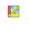
Figure 1: Phase-space picture corresponding to the construction in table 1.

In figure 1 we plot the phase-space representation of the sets of operators in table 1. Each set has been arbitrarily assigned to the number appearing in the left column of the table. The sets of operators 1 and 5 define the horizontal and the vertical axes, respectively, and they lead, together with the operators associated to line 2, to three separable bases (i.e., the three operators in each of the first three rows commute for each of the two subsystems, separately). In physical space, all these operators can be associated with rotations of each qubit around the $z$-, $x$- and $y$-axis, respectively. Eigenstates of the operators associated with the lines 3 and 4 form entangled bases (in fact, their simultaneous eigenstates are all maximally entangled states). The origin is labeled as $o$ and is the common intersecting point of all the rays.

It is clear that under local transformations the factorable and entangled MUBs preserve their separability properties. Two natural questions thus arise in this respect: Is the arrangement in table 1 and the corresponding geometrical association with rays in phase-space unique? If this is not the case, why do different arrangements always lead to the same separability structure of MUBs?

4 Curves in phase space

To answer these questions we shall approach the problem from a different perspective, namely, by determining all the possible geometrical structures in phase space that correspond to MUBs. First of all, let us observe that any ray can be defined in the parametric form

$$\alpha(\kappa)=\eta\kappa\,,\qquad\beta(\kappa)=\zeta\kappa\,,$$ (4.1)

where $\eta,\zeta\in GF(4)$ are fixed while $\kappa\in GF(4)$ is a parameter that runs through all the field elements. The rays (4.1) can be seen as the simplest nonsingular (i.e., no self-intersecting) Abelian substructures in phase space, in the sense that

$$\alpha(\kappa+\kappa^{\prime})=\alpha(\kappa)+\alpha(\kappa^{\prime})\,,\qquad\beta(\kappa+\kappa^{\prime})=\beta(\kappa)+\beta(\kappa^{\prime})\,.$$ (4.2)

However, the rays are not the only Abelian structures: it is easy to see that the parametric curves (that obviously pass through the origin)

$$\alpha(\kappa)=\mu_{0}\kappa+\mu_{1}\kappa^{2}\,,\qquad\beta(\kappa)=\eta_{0}\kappa+\eta_{1}\kappa^{2}\,,$$ (4.3)

also satisfy the condition (4.2). If, in addition, we impose

$$\tr(\alpha\beta^{\prime})=\tr(\alpha^{\prime}\beta)\,,$$ (4.4)

where $\alpha^{\prime}=\alpha(\kappa^{\prime})$ and $\beta^{\prime}=\beta(\kappa^{\prime})$, then the displacement operators associated to the curves (4.3) commute with each other and the coefficients $\mu_{j}$ and $\eta_{j}$ must satisfy the following restrictions (commutativity conditions)

$$\mu_{1}\eta_{0}+(\mu_{1}\eta_{0})^{2}=\mu_{0}\eta_{1}+(\mu_{0}\eta_{1})^{2}\,.$$ (4.5)

All the possible Abelian curves satisfying condition (4.5) can be divided into two types:

a) regular curves

$$\alpha\mathrm{-curves} : \quad\alpha=\sigma\kappa\,,\quad\beta=\eta\kappa+\sigma^{2}\kappa^{2}\,,$$

$$\beta\mathrm{-curves} : \quad\beta=\sigma\kappa\,,\quad\alpha=\eta\kappa+\sigma^{2}\kappa^{2}\,.$$

b) exceptional curves

$$\alpha=\mu(\kappa+\kappa^{2})\,,\quad\beta=\mu^{2}(\sigma\kappa+\sigma^{2}\kappa^{2})\,.$$ (4.7)

The regular curves are nondegenerate, in the sense that $\alpha$ or $\beta$ (or both) are not repeated in any set of four points defining a curve. In other words, $\alpha$ or $\beta$ (or both) take all the values in the field $GF(4)$. This allows us to write down explicit relations between $\alpha$ and $\beta$ as follows

$$\alpha\mathrm{-curves} : \quad\beta=\eta\sigma^{2}\alpha+\alpha^{2}\,,$$

$$\beta\mathrm{-curves} : \quad\alpha=\eta\sigma^{2}\beta+\beta^{2}\,.$$

By varying the parameter $\eta$ in the first of equations (4) we can construct the $\alpha$-curves in table 2, which show a different arrangement of operators than (3). Figure 2 shows the corresponding points of $\alpha$-curves in phase space. Note, that we have completed table 2 and figure 2 with the vertical ($X_{\sigma},X_{\sigma^{2}},X_{\sigma^{3}}$) axis. The factorization of operators in each table (the self-dual basis is used for the representation of operators in terms of Pauli matrices) is different from the standard one in table 1. The curves marked as 3, 4 and 5 lead now to factorable MUBs, while the ones marked as 1 and 2 lead to maximally entangled bases.

The $\beta$-curves and the corresponding table can be obtained from table 2 by exchanging $\alpha$ and $\beta$ (and correspondingly $Z$ and $X$ operators) and is given in table 3. The phase-space picture corresponding to table 3 is shown in figure 3 and can be easily obtained from figure 2 by mirroring this figure about the main diagonal. Observe that the curves $\beta=\alpha^{2}$ and $\alpha=\beta^{2}$ then become identical, since this curve is symmetric about the diagonal.

Table 2: $\alpha$-curves and their corresponding operators.

• Basis	$\alpha$-curves	Displacement operators	Factorized operators
  1	$\beta=\alpha^{2}$	$Z_{\sigma^{2}}X_{\sigma},Z_{\sigma^{3}}X_{\sigma^{3}},Z_{\sigma}X_{\sigma^{2}}$	$\sigma_{x}\sigma_{z}$	$\sigma_{y}\sigma_{y}$	$\sigma_{z}\sigma_{x}$
  2	$\beta=\alpha+\alpha^{2}$	$Z_{\sigma^{2}}X_{\sigma^{3}},Z_{\sigma^{3}},Z_{\sigma}X_{\sigma^{3}}$	$\sigma_{x}\sigma_{y}$	$\sigma_{z}\sigma_{z}$	$\sigma_{y}\sigma_{x}$
  3	$\beta=\sigma\alpha+\alpha^{2}$	$Z_{\sigma^{2}}X_{\sigma^{2}},Z_{\sigma^{3}}X_{\sigma^{2}},Z_{\sigma}$	$\leavevmode\hbox{\small 1\normalsize\kern-3.30002pt1}\sigma_{y}$	$\sigma_{z}\sigma_{y}$	$\sigma_{z}\leavevmode\hbox{\small 1\normalsize\kern-3.30002pt1}$
  4	$\beta=\sigma^{2}\alpha+\alpha^{2}$	$Z_{\sigma^{2}},Z_{\sigma^{3}}X_{\sigma},Z_{\sigma}X_{\sigma}$	$\leavevmode\hbox{\small 1\normalsize\kern-3.30002pt1}\sigma_{z}$	$\sigma_{y}\sigma_{z}$	$\sigma_{y}\leavevmode\hbox{\small 1\normalsize\kern-3.30002pt1}$
  5	$\alpha=0$	$X_{\sigma},X_{\sigma^{2}},X_{\sigma^{3}}$	$\sigma_{x}\leavevmode\hbox{\small 1\normalsize\kern-3.30002pt1}$	$\leavevmode\hbox{\small 1\normalsize\kern-3.30002pt1}\sigma_{x}$	$\sigma_{x}\sigma_{x}$

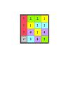
Figure 2: Phase-space picture corresponding to the construction in table 2.

Table 3: Phase-space $\beta$-curves and their corresponding operators.

• Basis	$beta$-curves	Displacement operators	Factorized operators
  1	$\alpha=\beta^{2}$	$X_{\sigma^{2}}Z_{\sigma},X_{\sigma^{3}}Z_{\sigma^{3}},X_{\sigma}Z_{\sigma^{2}}$	$\sigma_{z}\sigma_{x}$	$\sigma_{y}\sigma_{y}$	$\sigma_{x}\sigma_{z}$
  2	$\alpha=\beta+\beta^{2}$	$X_{\sigma^{2}}Z_{\sigma^{3}},X_{\sigma^{3}},X_{\sigma}Z_{\sigma^{3}}$	$\sigma_{z}\sigma_{y}$	$\sigma_{x}\sigma_{x}$	$\sigma_{y}\sigma_{z}$
  3	$\alpha=\sigma\beta+\beta^{2}$	$X_{\sigma^{2}}Z_{\sigma^{2}},X_{\sigma^{3}}Z_{\sigma^{2}},X_{\sigma}$	$\leavevmode\hbox{\small 1\normalsize\kern-3.30002pt1}\sigma_{y}$	$\sigma_{x}\sigma_{y}$	$\sigma_{x}\leavevmode\hbox{\small 1\normalsize\kern-3.30002pt1}$
  4	$\alpha=\sigma^{2}\beta+\beta^{2}$	$X_{\sigma^{2}},X_{\sigma^{3}}Z_{\sigma},X_{\sigma}Z_{\sigma}$	$\leavevmode\hbox{\small 1\normalsize\kern-3.30002pt1}\sigma_{x}$	$\sigma_{y}\sigma_{x}$	$\sigma_{y}\leavevmode\hbox{\small 1\normalsize\kern-3.30002pt1}$
  5	$\beta=0$	$Z_{\sigma},Z_{\sigma^{2}},Z_{\sigma^{3}}$	$\sigma_{z}\leavevmode\hbox{\small 1\normalsize\kern-3.30002pt1}$	$\leavevmode\hbox{\small 1\normalsize\kern-3.30002pt1}\sigma_{z}$	$\sigma_{z}\sigma_{z}$

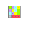
Figure 3: Phase-space picture corresponding to the construction in table 3.

It is worth noting that all the $\alpha$-curves, except $\beta=\alpha^{2}$, are $\beta$-degenerate: the same value of $\beta$ corresponds to different values of $\alpha$. Obviously, the analogous $\alpha$-degeneration appears in the $\beta$-curves.

Exceptional curves (4.7) have quite a different structure. Now, every point is doubly degenerate and can be obtained from equations that relate powers of $\alpha$ and $\beta$:

$$\alpha^{2}=\mu\alpha\,,\qquad\beta^{2}=\mu^{2}\beta\,.$$ (4.9)

It is impossible to write an explicit nontrivial equation of the form $f(\alpha,\beta)=0$ for them. The existence of these curves allows us to obtain interesting arrangements of MUB operators in tables that do not contain any axis ($z$, $x$ or $y$). There are two of such structures, shown in tables 4 and 5. As can be seen from the rightmost column in both tables, the physical difference between the two structures is that the two qubits are permuted between them. The lines marked 2, 3 and 4 in both tables lead to factorable MUBs, while the lines marked as 1 and 5 give maximally entangled ones.

Table 4: Bundle consisting of two exceptional curves, one $\alpha$-curve, one $\beta$-curve, and a ray.

• Basis	Curves and rays	Displacement operators	Factorized operators
  1	$\!\!\!\begin{array}[]{l}\alpha=\kappa+\kappa^{2}\\ \beta=\sigma\kappa+\sigma^{2}\kappa^{2}\end{array}$	$X_{\sigma^{3}},Z_{\sigma^{3}},Z_{\sigma^{3}}X_{\sigma^{3}}$	$\sigma_{x}\sigma_{x}$	$\sigma_{z}\sigma_{z}$	$\sigma_{y}\sigma_{y}$
  2	$\!\!\!\begin{array}[]{l}\alpha=\sigma^{2}(\kappa+\kappa^{2})\\ \beta=\sigma^{2}\kappa+\kappa^{2}\end{array}$	$X_{\sigma},Z_{\sigma^{2}},Z_{\sigma^{2}}X_{\sigma}$	$\sigma_{x}\leavevmode\hbox{\small 1\normalsize\kern-3.30002pt1}$	$\leavevmode\hbox{\small 1\normalsize\kern-3.30002pt1}\sigma_{z}$	$\sigma_{x}\sigma_{z}$
  3	$\beta=\sigma\alpha+\alpha^{2}$	$Z_{\sigma^{2}}X_{\sigma^{2}},Z_{\sigma^{3}}X_{\sigma^{2}},Z_{\sigma}$	$\leavevmode\hbox{\small 1\normalsize\kern-3.30002pt1}\sigma_{y}$	$\sigma_{z}\sigma_{y}$	$\sigma_{z}\leavevmode\hbox{\small 1\normalsize\kern-3.30002pt1}$
  4	$\alpha=\sigma^{2}\beta+\beta^{2}$	$X_{\sigma^{2}},Z_{\sigma}X_{\sigma^{3}},Z_{\sigma}X_{\sigma}$	$\leavevmode\hbox{\small 1\normalsize\kern-3.30002pt1}\sigma_{x}$	$\sigma_{y}\sigma_{x}$	$\sigma_{y}\leavevmode\hbox{\small 1\normalsize\kern-3.30002pt1}$
  5	$\beta=\sigma\alpha$	$Z_{\sigma}X_{\sigma^{2}},Z_{\sigma^{2}}X_{\sigma^{3}},Z_{\sigma^{3}}X_{\sigma}$	$\sigma_{z}\sigma_{x}$	$\sigma_{x}\sigma_{y}$	$\sigma_{y}\sigma_{z}$

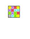
Figure 4: Phase-space picture corresponding to the construction in table 4.

Table 5: Bundle consisting of two exceptional curves, one $\alpha$-curve, one $\beta$-curve, and a ray.

• Basis	Curves and rays	Displacement operators	Factorized operators
  1	$\!\!\!\begin{array}[]{l}\alpha=\kappa+\kappa^{2}\\ \beta=\sigma\kappa+\sigma^{2}\kappa^{2}\end{array}$	$X_{\sigma^{3}},Z_{\sigma^{3}},Z_{\sigma^{3}}X_{\sigma^{3}}$	$\sigma_{x}\sigma_{x}$	$\sigma_{z}\sigma_{z}$	$\sigma_{y}\sigma_{y}$
  2	$\!\!\!\begin{array}[]{l}\alpha=\sigma(\kappa+\kappa^{2})\\ \beta=\kappa+\sigma\kappa^{2}\end{array}$	$X_{\sigma^{2}},Z_{\sigma},Z_{\sigma}X_{\sigma^{2}}$	$\leavevmode\hbox{\small 1\normalsize\kern-3.30002pt1}\sigma_{x}$	$\sigma_{z}\leavevmode\hbox{\small 1\normalsize\kern-3.30002pt1}$	$\sigma_{z}\sigma_{x}$
  3	$\beta=\sigma^{2}\alpha+\alpha^{2}$	$Z_{\sigma^{2}},Z_{\sigma^{3}}X_{\sigma},Z_{\sigma}X_{\sigma}$	$\leavevmode\hbox{\small 1\normalsize\kern-3.30002pt1}\sigma_{z}$	$\sigma_{y}\sigma_{z}$	$\sigma_{y}\leavevmode\hbox{\small 1\normalsize\kern-3.30002pt1}$
  4	$\alpha=\sigma\beta+\beta^{2}$	$Z_{\sigma^{2}}X_{\sigma^{2}},Z_{\sigma^{2}}X_{\sigma^{3}},X_{\sigma}$	$\leavevmode\hbox{\small 1\normalsize\kern-3.30002pt1}\sigma_{y}$	$\sigma_{x}\sigma_{y}$	$\sigma_{x}\leavevmode\hbox{\small 1\normalsize\kern-3.30002pt1}$
  5	$\beta=\sigma^{2}\alpha$	$Z_{\sigma}X_{\sigma^{3}},Z_{\sigma^{2}}X_{\sigma},Z_{\sigma^{3}}X_{\sigma^{2}}$	$\sigma_{y}\sigma_{x}$	$\sigma_{x}\sigma_{z}$	$\sigma_{z}\sigma_{y}$

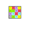
Figure 5: Phase-space picture corresponding to the construction in table 5.

Finally, there is a last table containing two exceptional curves and a ray corresponding to the spin operators in the $y$-direction, as it is shown in table 6.

To sum up, there exist fifteen different Abelian structures, five rays and ten curves, which can be organized in six different forms with the respect to MUBs. The existence of only six bundles of mutually nonintersecting Abelian nonsingular curves (i.e., different tables) also follows from the fact that the coset of the full symplectic group, which preserves the commutation relations (2.7), on operations corresponding to nontrivial permutations of columns and rows of (any) table [generated by the symplectic group $Sp(2,GF(4))$], is precisely of order 6.

Table 6: Bundle consisting of two exceptional curves, one $\alpha$-curve, one $\beta$-curve, and a ray.

• Basis	Curves and rays	Displacement operators	Factorized operators
  1	$\!\!\!\begin{array}[]{l}\alpha=\sigma^{2}(\kappa+\kappa^{2})\\ \beta=\sigma^{2}\kappa+\kappa^{2}\end{array}$	$X_{\sigma^{2}},Z_{\sigma},Z_{\sigma}X_{\sigma^{2}}$	$\leavevmode\hbox{\small 1\normalsize\kern-3.30002pt1}\sigma_{x}$	$\sigma_{z}\leavevmode\hbox{\small 1\normalsize\kern-3.30002pt1}$	$\sigma_{z}\sigma_{x}$
  2	$\!\!\!\begin{array}[]{l}\alpha=\sigma(\kappa+\kappa^{2})\\ \beta=\sigma\kappa+\sigma\kappa^{2}\end{array}$	$X_{\sigma},Z_{\sigma^{2}},Z_{\sigma^{2}}X_{\sigma}$	$\sigma_{x}\leavevmode\hbox{\small 1\normalsize\kern-3.30002pt1}$	$\leavevmode\hbox{\small 1\normalsize\kern-3.30002pt1}\sigma_{z}$	$\sigma_{x}\sigma_{z}$
  3	$\beta=\alpha+\alpha^{2}$	$Z_{\sigma^{2}}X_{\sigma^{3}},Z_{\sigma^{3}},Z_{\sigma}X_{\sigma^{3}}$	$\sigma_{y}\sigma_{x}$	$\sigma_{z}\sigma_{z}$	$\sigma_{x}\sigma_{y}$
  4	$\alpha=\beta+\beta^{2}$	$Z_{\sigma^{3}}X_{\sigma^{2}},X_{\sigma^{3}},Z_{\sigma^{3}}X_{\sigma}$	$\sigma_{z}\sigma_{y}$	$\sigma_{x}\sigma_{x}$	$\sigma_{y}\sigma_{z}$
  5	$\beta=\alpha$	$Z_{\sigma}X_{\sigma},Z_{\sigma^{2}}X_{\sigma^{2}},Z_{\sigma^{3}}X_{\sigma^{3}}$	$\sigma_{y}\leavevmode\hbox{\small 1\normalsize\kern-3.30002pt1}$	$\leavevmode\hbox{\small 1\normalsize\kern-3.30002pt1}\sigma_{y}$	$\sigma_{y}\sigma_{y}$

5 The effect of local transformations

As we have noticed, different arrangements of operators in tables (or bundling of phase-space curves) lead to the same separability structure. To understand this point, let us study the effect of local transformations. In other words, we wish to characterize how a given curve changes when a local transformation is applied to a set of operators labeled by points of this curve.

To deal with such operations with curves, let us recall that a generic displacement operator is factorized in the self-dual basis as

$$Z_{\alpha}X_{\beta}=(\sigma_{z}^{a_{1}}\sigma_{x}^{b_{1}})(\sigma_{z}^{a_{2}}\sigma_{x}^{b_{2}})\equiv(a_{1},b_{1})\otimes(a_{2},b_{2})\,.$$ (5.1)

It is clear that under local transformation (rotations by $\pi/2$ radians around the $z$-, $x$- or $y$-axes) applied to the $j$th particle ($j=1,2$), the indices of the displacement operators are transformed as follows:

$$z\mathrm{-rotation} : \quad(a_{j},b_{j})\rightarrow(a_{j}+b_{j},b_{j})\,,$$

$$x\mathrm{-rotation} : \quad(a_{j},b_{j})\rightarrow(a_{j},b_{j}+a_{j})\,,$$ (5.2)

$$y\mathrm{-rotation} : \quad(a_{j},b_{j})\rightarrow(a_{j}+a_{j}+b_{j},b_{j}+a_{j}+b_{j})=(b_{j},a_{j})\,.$$

To give a concrete example, suppose we consider a $z$-axis rotation. The operator $\sigma_{z}$, corresponding to $(a_{j}=1,b_{j}=0)$, is transformed into $(a_{j}=1+0=1,b_{j}=0)$; i.e., into itself, while, e.g., the operator $\sigma_{x}$, corresponding to $(a_{j}=0,b_{j}=1)$, is mapped onto $(a_{j}=0+1=1,b_{j}=1)$, which coincides with $\sigma_{y}$. In the same way $\sigma_{y}$ is mapped onto $\sigma_{x}$, while the identity ($a_{j}=0$, $b_{j}=0$) is mapped onto itself.

In terms of field elements these transformations read

$$z\mathrm{-rotation} : \quad\begin{array}[]{l}\alpha\rightarrow\alpha+\theta_{j}\tr(\beta\theta_{j}),\\ \beta\rightarrow\beta,\end{array}$$ (5.5)

$$x\mathrm{-rotation} : \quad\begin{array}[]{l}\alpha\rightarrow\alpha,\\ \beta\rightarrow\beta+\theta_{j}\tr(\alpha\theta_{j}),\end{array}$$ (5.8)

$$y\mathrm{-rotation} : \quad\begin{array}[]{l}\alpha\rightarrow\alpha+\theta_{j}\tr[(\alpha+\beta)\theta_{j}],\\ \beta\rightarrow\beta+\theta_{j}\tr[(\alpha+\beta)\theta_{j}].\end{array}$$ (5.11)

In particular, applying the above transformations to a ray (4.1) we get

$$z\mathrm{-rotation} : \quad\begin{array}[]{l}\alpha\rightarrow(\eta+\zeta\theta_{j})\kappa+\kappa^{2}\zeta^{2},\\ \beta\rightarrow\beta=\zeta\kappa,\end{array}$$ (5.14)

$$x\mathrm{-rotation} : \quad\begin{array}[]{l}\alpha\rightarrow\alpha=\eta\kappa,\\ \beta\rightarrow(\zeta+\eta\theta_{j})\kappa+\kappa^{2}\eta^{2},\end{array}$$ (5.17)

$$y\mathrm{-rotation} : \quad\begin{array}[]{l}\alpha\rightarrow(\eta+\zeta\theta_{j}+\eta\theta_{j})\kappa+\kappa^{2}(\zeta+\eta)^{2},\\ \beta\rightarrow(\zeta+\zeta\theta_{j}+\eta\theta_{j})\kappa+\kappa^{2}(\zeta+\eta)^{2},\end{array}$$ (5.20)

which are explicitly nonlinear operations.

Note that the $z$- and $x$-transformations produce regular curves starting from a ray

$$z\mathrm{-rotation} : \quad\alpha=\eta\zeta^{-1}\beta\rightarrow(\eta\zeta^{-1}+\theta_{j})\beta+\beta^{2},$$

$$x\mathrm{-rotation} : \quad\beta=\eta^{-1}\zeta\alpha\rightarrow(\eta^{-1}\zeta+\theta_{j})\alpha+\alpha^{2}.$$

Meanwhile, the $y$-rotation may lead to an exceptional curve (as it happens when we start with the horizontal or the vertical axes, $\zeta=0$ or $\eta=0$).

An important result to stress is that it is possible to obtain all the curves of the form (4) and (4.7) from the rays after some (nonlinear) operations (5.14), corresponding to local transformations. The families of such transformations are the following:

I. The rays and curves corresponding to factorable basis can be obtained from a single ray $\alpha=0,\beta=\sigma^{2}\kappa$ (vertical axis) as shown in table 7 (left).

II. The rays and curves corresponding to nonfactorable basis can be obtained from the ray $\alpha=\sigma\kappa,\beta=\sigma^{2}\kappa$ ($\beta=\sigma\alpha)$ as shown in table 7 (right).

Table 7: Curves and their corresponding transformations from $\alpha=0,\beta=\sigma^{2}\kappa$ (left) and $\beta=\sigma\alpha$ (right). The $x$-, $y$ and $z$-rotations are indicated as $x$, $y$ and $z$, respectively.

• Curve (ray)	Transformation	Curve (ray)	Transformation
  $\!\!\!\begin{array}[]{l}\alpha=\sigma^{2}(\kappa+\kappa^{2})\\ \beta=\sigma^{2}\kappa+\kappa^{2}\end{array}$	$\leavevmode\hbox{\small 1\normalsize\kern-3.30002pt1}\otimes y$	$\!\!\!\begin{array}[]{l}\alpha=\kappa+\kappa^{2}\\ \beta=\sigma\kappa+\sigma^{2}\kappa^{2}\end{array}$	$z\otimes y$
  $\!\!\!\begin{array}[]{l}\alpha=\sigma(\kappa+\kappa^{2})\\ \beta=\sigma\kappa+\sigma\kappa^{2}\end{array}$	$y\otimes\leavevmode\hbox{\small 1\normalsize\kern-3.30002pt1}$	$\beta=\sigma^{2}\alpha$	$x\otimes x$
  $\beta=0$	$y\otimes y$	$\beta=\alpha^{2}$	$\leavevmode\hbox{\small 1\normalsize\kern-3.30002pt1}\otimes x$
  $\beta=\alpha$	$z\otimes z$	$\beta=\alpha+\alpha^{2}$	$\leavevmode\hbox{\small 1\normalsize\kern-3.30002pt1}\otimes y$
  $\beta=\sigma\alpha+\alpha^{2}$	$y\otimes z$	$\alpha=\beta+\beta^{2}$	$y\otimes\leavevmode\hbox{\small 1\normalsize\kern-3.30002pt1}$
  $\beta=\sigma^{2}\alpha+\alpha^{2}$	$z\otimes y$
  $\alpha=\sigma\beta+\beta^{2}$	$\leavevmode\hbox{\small 1\normalsize\kern-3.30002pt1}\otimes z$
  $\alpha=\sigma^{2}\beta+\beta^{2}$	$z\otimes\leavevmode\hbox{\small 1\normalsize\kern-3.30002pt1}$

This means that all the different tables can be generated from the standard one, given in table 1, by applying only local transformations that do not change the factorization properties of the MUBs. So, tables 2 to 6 are obtained from table 1 from the transformations given in table 8.

The full set of striations for each bundle of curves (each table) is obtained by constructing “parallel curves” in the bundle in an obvious way:

$$\alpha_{\lambda}(\kappa)=\mu_{0}\kappa+\mu_{1}\kappa^{2},\qquad\beta_{\lambda}(\kappa)=\eta_{0}\kappa+\eta_{1}\kappa^{2}+\lambda,$$ (5.22)

with $\lambda\in GF(4)$. It is clear that no ($\alpha_{\lambda}(\kappa),\beta_{\lambda}(\kappa)$) curve intersects the curve ($\alpha_{\lambda^{\prime}}(\kappa),\beta_{\lambda^{\prime}}(\kappa)$) for $\lambda\neq\lambda^{\prime}$.

6 Extension to larger spaces

The relation between Abelian curves in discrete phase space and different systems of MUBs can be extended to higher (power of prime) dimensions. For the most interesting $n$-qubit case, a generic Abelian curve (4.2) has the following parametric from

$$\alpha(\kappa)=\sum_{m=0}^{n-1}\mu_{m}\kappa^{2^{m}}\,,\qquad\beta(\kappa)=\sum_{m=0}^{n-1}\eta_{m}\kappa^{2^{m}}\,,$$ (6.1)

with $\mu_{m},\eta_{m},\kappa\in GF(2^{n})$, and the commutativity condition takes now the invariant form

$$\sum_{m\neq k}\tr(\mu_{m}\mathbf{\eta}_{k})=0\,.$$ (6.2)

The simplest example of such curves are obviously the rays, parametrically defined as in Eq. (4.1), where the conditions (6.2) are trivially satisfied. Imposing the nonintersecting condition we can, in principle, get all the possible bundles of commutative curves. Nevertheless, in higher dimensions it is impossible to obtain all the curves from the rays by local transformations. This leads to the existence of different nontrivial bundles of nonintersecting curves, and consequently to MUBs with different types of factorization [22, 36].

The problem of classification of bundles of mutually nonintersecting, nonsingular Abelian curves and its relation to the problem of MUBs in higher dimensions, and in particular the transformation relations between different MUB structures, will be considered elsewhere.

Table 8: Transformation operators converting table 1 into each one of the tables indicated in the left column. Again, $x$-, $y$- and $z$-rotations are indicated as $x$, $y$ and $z$, respectively.

• Table	Transformation
  2	$x\otimes\leavevmode\hbox{\small 1\normalsize\kern-3.30002pt1}$
  3	$\leavevmode\hbox{\small 1\normalsize\kern-3.30002pt1}\otimes z$
  4	$y\otimes z$
  5	$y\otimes x$
  6	$\leavevmode\hbox{\small 1\normalsize\kern-3.30002pt1}\otimes y$

7 Conclusions

A new MUB construction has been worked out, with special emphasis in the two-qubit case. Its essential ingredient is a mapping between displacement operators, physical spin-1/2 operators and discrete phase-space curves. In phase space any nonsingular bundle of curves that fills every point and has only one common intersecting point (here taken to be the origin) will map onto a MUB. The corresponding displacement operators can be obtained from these phase-space curves.

For the two-qubit case, we have derived all the admissible curves and classified them into rays and curves (regular and exceptional, depending on degeneracy). In total, six different bundles can be constructed from the set of five rays and ten curves. We have also shown how the six tables representing sets of MUBs are related by local transformations, i.e., physical rotations around the $x$-, $y$- and $z$-axes. It is obvious that such rotations will not change the MUBs entanglement properties.

A Wigner function can also be associated to each phase-space structure. Although we have not pursued this topic in the paper, it is straightforward to use any of the phase-space structures and follow the algorithm described in reference [33] (although in that paper the construction applies only to rays) to obtain such a function [39].

It is also formally straightforward to extend the method to any Hilbert space whose dimension is a power of a prime. However, only in the bipartite case one will find that all structures are related through local transformations. Already in the tripartite case different classes of entanglement exist [36], and consequently some MUB structures are related through nonlocal (entangling) transformations. The extention of the present method provides a systematic way to find these transformations.

8 Acknowledgements

This work was supported by the Grant 45704 of Consejo Nacional de Ciencia y Tecnologia (CONACyT), Mexico, the Swedish Foundation for International Cooperation in Research and Higher Education (STINT), the Swedish Research Council (VR), the Swedish Foundation for Strategic Research (SSF), and the Spanish Research Directorate (DGI), Grant FIS2005-0671.

References

- [1] Schwinger J 1960 Proc. Natl. Acad. Sci. USA 46 570
- [2] Wootters W K 1987 Ann. Phys. (NY) 176 1
- [3] Kraus K 1987 Phys. Rev. D 35 3070
- [4] Lawrence J, Brukner Č and Zeilinger A 2002 Phys. Rev. A 65 032320
- [5] Chaturvedi S 2002 Phys. Rev. A 65 044301
- [6] Wootters W K 2006 Found. Phys. 36 112
- [7] Wootters W K and Fields B D 1989 Ann. Phys. (NY) 191 363
- [8] Asplund R and Björk G 2001 Phys. Rev. A 64 012106
- [9] Bechmann-Pasquinucci H and Peres A 2000 Phys. Rev. Lett. 85 3313
- [10] Cerf N, Bourennane M, Karlsson A and Gisin N 2002 Phys. Rev. A 88 127902
- [11] Gottesman D 1996 Phys. Rev. A 54 1862
- [12] Calderbank A R, Rains E M, Shor P W and Sloane N J A 1997 Phys. Rev. Lett. 78 405
- [13] Vaidman L, Aharonov Y and Albert D Z 1987 Phys. Rev. Lett. 58 1385
- [14] Englert B.-G and Aharonov Y 2001 Phys. Lett. A 284 1
- [15] Aravind P K 2003 Z. Naturforschung. A 26 350
- [16] Schulz O, Steinhübl R, Weber M, Englert B.-G, Kurtsiefer C and Weinfurter H 2003 Phys. Rev. Lett. 90 177901
- [17] Kimura G, Tanaka H and Ozawa M 2006 Phys. Rev. A 73 050301(R)
- [18] Ivanovic I D 1981 J. Phys. A: Math. Gen. 14 3241
- [19] Calderbank A R, Cameron P J, Kantor W M and Seidel J J 1997 Proc. London Math. Soc. 75 436
- [20] Bandyopadhyay S, Boykin P O, Roychowdhury V and Vatan V 2002 Algorithmica 34 512
- [21] Klappenecker A and Rötteler M 2004 Lecture Notes in Comput. Sci. 2948 137
- [22] Lawrence J 2004 Phys. Rev. A 70 012302
- [23] Parthasarathy K R 2004 Infin. Dimens. Anal. Quantum Probab. Relat. Top. 7 607
- [24] Pittenger A O and Rubin M H 2005 J. Phys. A: Math. Gen. 38 6005
- [25] Durt T 2005 J. Phys. A: Math. Gen. 38 5267
- [26] Planat M and Rosu H 2005 Eur. Phys. J. D 36 133
- [27] Klimov A B, Sánchez-Soto L L and de Guise H 2005 J. Phys. A: Math. Gen. 38 2747
- [28] Lidl R and Niederreiter H 1986 Introduction to Finite Fields and their Applications (Cambridge: Cambridge University Press)
- [29] Buot F A 1974 Phys. Rev. B 10 3700
- [30] Galetti D and De Toledo Piza A F R 1988 Physica A 149 267
- [31] Cohendet O, Combe Ph, Sirugue M and Sirugue-Collin M 1988 J. Phys. A: Math. Gen. 21 2875
- [32] Wootters W K 2004 IBM J. Res. Dev. 48 99
- [33] Gibbons K S, Hoffman M J and Wootters W K 2004 Phys. Rev. A 70 062101
- [34] Paz J P, Roncaglia A J and Saraceno M 2005 Phys. Rev. A 72 012309
- [35] Durt T 2006 Open Syst. Inf. Dyn. 13 403
- [36] Romero J L, Björk G, Klimov A B and Sánchez-Soto L L 2005 Phys. Rev. A 72 062310
- [37] Vourdas A 2004 Rep. Prog. Phys. 67 267
- [38] Englert B-G and Metwally N 2000 J. Mod. Opt. 47 2221
- [39] Björk G, Romero J L, Klimov A B and Sánchez-Soto L L 2007 J. Opt. Soc. Am. B 24 371