The Tidal Tails of NGC 5466

Abstract

The study of substructure in the stellar halo of the Milky Way has made a lot of progress in recent years, especially with the advent of surveys like the Sloan Digital Sky Survey. Here, we study the newly discovered tidal tails of the Galactic globular cluster NGC 5466. By means of numerical simulations, we reproduce the shape, direction and surface density of the tidal tails, as well as the structural and kinematical properties of the present-day NGC 5466. Although its tails are very extended in SDSS data $(\mathrel{\hbox to0.0pt{\lower 3.0pt\hbox{$\mathchar 536\relax$}\hss}\raise 2.0pt\hbox{$\mathchar 318\relax$}}45^{\circ}$), NGC 5466 is only losing mass slowly at the present epoch and so can survive for probably a further Hubble time. The tidal shaping through the Milky Way potential, especially the potential of the disc, is the dominant process in the slow dissolution of NGC 5466 accounting for $\mathrel{\hbox to0.0pt{\lower 3.0pt\hbox{$\mathchar 536\relax$}\hss}\raise 2.0pt\hbox{$\mathchar 318\relax$}}60\%$ of the mass loss over the course of its evolution. The morphology of the tails provides a constraint on the proper motion – the observationally determined proper motion has to be refined (within the stated error-margin) to match the location of the tidal tails.

1 Introduction

Within the last few years, it has become more and more obvious that the Milky Way stellar halo is dominated by substructure, particularly dwarf galaxies, clouds, and tidal tails. Data from the Sloan Digital Sky Survey (SDSS; York et al., 2000) have revealed abundant examples of streams and substructure. For example, Belokurov et al. (2006b) used a simple colour cut $g-r<0.4$ to map out the distribution of stars in SDSS Data Release 5 (DR5). The “Field of Streams”, an RGB-composite image composed of magnitude slices of the stellar density of these stars, showed the overlap of the leading and trailing arm of the well-known Sagittarius stream and the Monoceros ring very clearly. Also prominent was a new stream, which did not have an identified progenitor, and was called the “Orphan Stream” by Belokurov et al. (2006b). The observational data on the Orphan Stream (Belokurov et al., 2007) was used by Fellhauer et al. (2007) to argue that its progenitor may be the newly-discovered disrupting dwarf galaxy UMa II (Zucker et al., 2006).

Tidal tails have proved to be an important diagnostic of the Galactic potential. Especially the tails of the dissolving Sagittarius dwarf galaxy (see e.g. Ibata, Gilmore & Irwin, 1994; Majewski et al., 2003; Helmi, 2004; Johnston, Law & Majewski, 2005), which wrap around the Milky Way, are an excellent tracer of the strength and shape of the potential. Fellhauer et al. (2006) have shown with their numerical models that the bifurcation of the Sagittarius stream as seen in the “Field of Streams” is composed of two wraps of the tidal tails and can only be reproduced if the orbital precession is small, i.e. if the Milky Way dark matter halo is close to spherical.

Extra-tidal extensions and onsets of tidal tails have been claimed around a number of Galactic globular clusters in recent years (see e.g. Meylan, Leon & Combes, 2001). The most spectacular and convincing discovery remains the long and thin tail from the disrupting globular cluster Pal 5 (Odenkirchen et al., 2001; Rockosi et al., 2002; Odenkirchen et al., 2003). The tails extend at least $4$ kpc from the cluster in the leading and trailing direction and contain more mass than the remaining cluster.

Recently, two different groups (Belokurov et al., 2006a; Grillmair & Johnson, 2006) claim to have detected tidal tails of various extents around the disrupting globular cluster NGC 5466. This is an old, metal-poor ([Fe/H]$=-2.22$) cluster, lying at Galactic coordinates $l=42.\!\!^{o}15$, $b=73.\!\!^{o}59$. In Belokurov et al. (2006a), the observed tails of NGC 5466 are not as long as those of Pal 5, stretching about $2^{\circ}$ or $500$ pc in either direction. Grillmair & Johnson (2006) reported afterwards that they found evidence for a much larger extension of the tidal tails of NGC 5466. They claimed that the leading arm extends over $\sim 30$ degrees and the trailing arm extends at least $15$ degrees, before it leaves the area covered by SDSS. This finding makes the tails of NGC 5466 even longer, but much fainter, than the tails of Pal 5. The aim of our paper is to confront these claims with theoretical expectation, as well as to study the survival of the tails.

The following data for NGC 5466 are taken from various sources in the literature (Harris, 1996; Dinescu, Girard & van Altena, 1999; Lehmann & Scholz, 1997; Pryor et al., 1991). The central surface brightness is $21.28$ mag arcsec^-2. The total luminosity is $M_{V}=-6.96$ mag and the mass-to-light ratio as given by Pryor et al. (1991) is $\sim 1$. Using these values, we derive a total mass of about $5\times 10^{4}$ M_⊙. The core radius has values ranging from $6.1$ to $7.6$ pc; the half-mass radius ranges from $10.4$ to $13.1$ pc. The most substantial differences in the literature occur for the tidal radius. Here, values are spread between $61$ and $158$ pc. We use this data as constraints on our numerical simulations. Our aim is to access possible initial models of this globular cluster and analyse its stability and evolution in different sets of Milky Way potentials.

In the next section, we describe the setup of our simulations – namely, the choice of Galactic potential models, the orbit of NGC 5466 and finally the initial model of the cluster itself. This is followed by a study of the relative importance of two-body relaxation and disc shocking in Section 3, justifying our use of particle-mesh simulations in this paper. Then, in Section 4, we present simulations that reproduce the shape, extent and surface density of the tidal tails detected by Belokurov et al. (2006a) and Grillmair & Johnson (2006). The properties of the remnant and shown to correspond to the present-day NGC 5466. Finally, we examine how the tidal tails change as a function of the proper motion and hence orbit.

2 Setup

2.1 Galactic Models

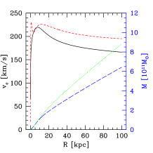
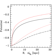
Figure 1: Comparison of the Galactic potentials. Left: Circular velocity of the ML (solid, black) and DB (dashed, red) potentials. Also plotted is the enclosed mass (right hand $y$-axis) of the ML (dotted, green) and DB (long-dashed, blue) models. Both potentials have the same circular velocity ($220$ km s^-1) at the solar radius. Right: Gravitational potential in the disc plane for the ML (dashed) and DB (solid) models. Also shown is the gravitational potential along the $z$-axis at the solar radius for the ML (dotted) and DB (long-dashed) models. Even though the potentials agree well in the innermost part, the ML potential is much steeper in the outer parts.

Dynamical friction does not play a significant role in the evolution of a low-mass star cluster. So, we are able to model the Galactic tidal field as a smooth and analytic background potential. For the Galactic potential, we use one of two standard models. The first (hereafter ML from (M)iamoto-Nagai + (L)ogarithmic halo) is a superposition of three components. The halo is represented by a spherical logarithmic potential of the form

$$\Phi_{\rm halo}(r) = {1\over 2}v_{0}^{2}\ln\left(1+\frac{r^{2}}{d^{2}}\right),$$ (1)

with $v_{0}=256$ km s^-1 and $d=12$ kpc (and $r$ is the spherical radius). The Galactic disc is modelled by a Miyamoto-Nagai potential:

$$\Phi_{\rm disc}(R,z) = -\frac{GM_{\rm d}}{\sqrt{R^{2}+\left(b+\sqrt{z^{2}+c^{2}}\right)^{2}}},$$ (2)

with $M_{\rm d}=10^{11}$ M_⊙, $b=6.5$ kpc and $c=0.26$ kpc (where $R$ and $z$ are cylindrical coordinates). The bulge is represented by a Hernquist potential

$$\Phi_{\rm bulge}(r) = -\frac{GM_{\rm b}}{r+a},$$ (3)

using $M_{\rm b}=3.4\times 10^{10}$ M_⊙ and $a=0.7$ kpc.

For comparison, we also use the Galactic potential suggested by Dehnen & Binney (1998) and hereafter denoted by DB. It consists of three disc components, namely the ISM, the thin and the thick disc, each of the form

$$\rho_{\rm disc}(R,z) = \frac{\Sigma_{\rm d}}{2z_{\rm d}}\exp\left(-\frac{R_{\rm m}}{R}-\frac{R}{R_{\rm d}}-\frac{|z|}{z_{\rm d}}\right).$$ (4)

With $R_{\rm m}=0$, Eq. (4) describes a standard double exponential disc with scale-length $R_{\rm d}$, scale-height $z_{\rm d}$ and central surface-density $\Sigma_{\rm d}$. For the stellar discs, $R_{\rm m}$ is set to be zero, while for the ISM-disc, we allow for a central depression by setting $R_{\rm m}=4$ kpc (Dehnen & Binney, 1998). In addition to the the disc potential, we use the analytic potential corresponding to two spheroidal density distributions for the halo and the bulge in the form

$$\rho(R,z) = \rho_{0}\left(\frac{m}{r_{0}}\right)^{-\gamma}\left(1+\frac{m}{r_{0}}\right)^{\gamma-\beta}\exp\left(-\frac{m^{2}}{r_{\rm t}^{2}}\right),$$ (5)

where

$$m = \sqrt{R^{2}+\frac{z^{2}}{q^{2}}}.$$ (6)

We choose the parameters of our DB model according to the best-fit model 4 in the paper of Dehnen & Binney (1998). In Fig. 1, we compare the two potentials. For both, the circular velocity at the solar radius is $220$ km s^-1. However, the ML model contains more mass within a given radius than the DB model.

2.2 Initial Model and Orbit for NGC 5466

As a initial model for the star cluster, we choose a Plummer (1911) sphere:

$$\rho(r) = \frac{3M_{\rm pl}}{4\pi R_{\rm pl}^{3}}\left(1+\frac{r^{2}}{R_{\rm pl}^{2}}\right)^{-5/2},$$ (7)

with $R_{\rm pl}$ being the scale-length of the Plummer sphere, which is identical to the half-light radius, and $M_{\rm pl}$ the total mass. This is a fairly good representation of a star cluster, especially a young one. However, due to tidal shaping and internal evolution at later stages, a King (1966) model usually fits the photometric data better. The advantage of a Plummer model is that all physical quantities are analytically accessible.

The initial Plummer model has a half-light radius of $10$ pc, an initial mass of $7\times 10^{4}$ M_⊙ and is represented by $10^{6}$ particles. The numerical set-up of the particles is performed using the algorithm of Aarseth, Henon & Wielen (1974). We checked that our initial model is able to survive for a Hubble time by comparing our initial configuration with the dissolution times given in Baumgardt & Makino (2003) (see their fig. 3). As the orbit of NGC 5466 is most of the time located far out in the halo, it is well represented by the uppermost lines in Baumgardt & Makino (2003), giving us a dissolution time of a few Hubble times.

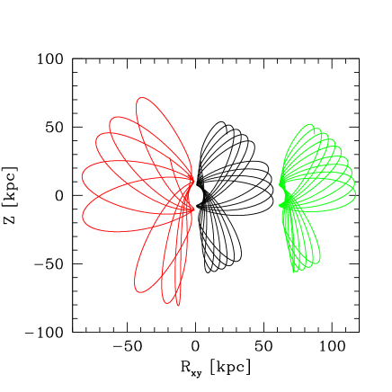
Figure 2: Comparison between the two orbits using the observationally determined proper motion. Left side (red): flipped orbit in the DB potential. Right side (black): orbit in the ML potential. The orbit with the revised proper motions in the ML potential is shown in green with an off-set of $+60$ kpc.

To determine the orbit of NGC 5466, we use the positions and proper motion from the literature (Harris, 1996; Dinescu et al., 1999), namely:

$$\alpha = 14^{\rm h}\ 05^{\rm m}\ 27^{\rm s}\!\!.3\ =\ 211.\!\!^{o}36$$

$$\delta = +28^{o}\ 32^{\prime}\ 04^{\prime\prime}\ =\ 28.\!\!^{o}53$$

$$D_{\odot} = 15.9\ {\rm kpc}$$

$$\mu_{\alpha}\cos\delta = -4.65\pm 0.82\ {\rm mas}\,{\rm yr}^{-1}$$

$$\mu_{\delta} = 0.80\pm 0.82\ {\rm mas}\,{\rm yr}^{-1}$$

$$v_{\rm rad} = 119.7\ {\rm km}\,{\rm s}^{-1}.$$

Its Galactocentric distance is $R_{\rm GC}=16.2$ kpc. We transform the positions and velocities into a Galactocentric Cartesian coordinate system and integrate a test particle back in time for $10$ Gyr. This endpoint of the backward-integration is then the starting position of our initial model. Even though the two potentials are quite similar in the innermost parts, the orbits differ in terms of perigalacticon, apogalacticon and number of disc crossings. In the DB potential, the Galaxy is less massive in the outer parts, so the cluster can reach an apogalacticon of $84$ kpc, while in the ML case, it only reaches $57$ kpc. The perigalactica are $5$ and $6$ kpc, respectively. In Fig. 2, the shape of the orbits in the $R$,$z$-plane is plotted (for the DB model, we flipped the radial coordinate onto the negative side to aid visibility).

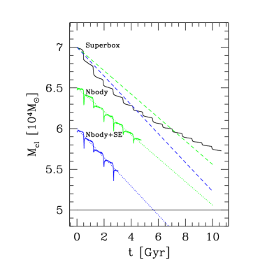
Figure 3: Bound mass versus time. Results of the NBODY 4 simulations in comparison with the Superbox particle-mesh simulations. The uppermost curve is the bound mass in the Superbox simulation. The results of the NBODY 4 simulations have been shifted downwards by $0.5$ and $1.0$ times $10^{4}$ M_⊙, respectively for clarity. The middle curve (green) shows the result of the NBODY 4 simulation neglecting stellar evolution and lowest curve (blue) shows the result of the NBODY 4 run with stellar evolution. Shown are also the linear fitting lines to the NBODY 4 results (dashed lines).

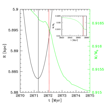
Figure 4: Mass-loss at one perigalacticon and disc-passage of the particle-mesh simulation in a more detailed time resolution. The (black) parabolic curve shows the distance to the centre of the MW with the first (black) vertical line showing the time of perigalacticon. The second (red) vertical line shows the time of the actual disc crossing ($z=0$). The (green) curve together with the right ordinate shows the evolution of the bound mass. It is visible in this figure that the mass-loss ceases after perigalacticon and turns into a steep mass-loss at the disc crossing. But as shown in the in-set (vertical lines are the same as in the main figure) the total mass-loss at this combination of perigalacticon and disc passage is $6$ times larger than the steep mass-loss caused by the actual disc passage.

3 Justification of Particle-Mesh Simulations

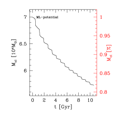
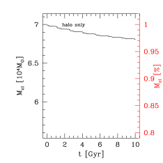
Figure 5: Mass-loss of NGC 5466 in the DB potential (left panel), in the ML potential (middle left panel), in the ML potential with the revised proper motions (middle right panel) and in the halo only potential (right panel).

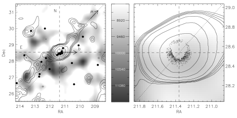
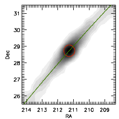
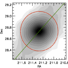
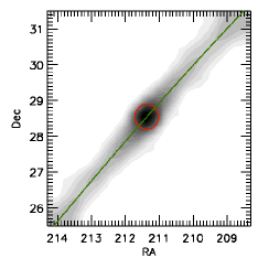
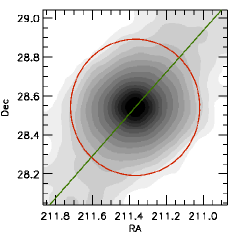
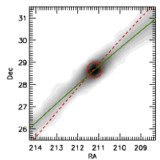
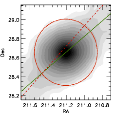
Figure 6: Contour plots of the tails (the model contours have logarithmic spacing). The solid green line shows the actual orbit; the red circle the size of the actual tidal radius. Top left: Observations using SDSS by Belokurov et al. (2006a). Top right: Simulation using the DB potential. Lower left: ML potential. Lower right: ML potential combined with the revised proper motion. The tidal tails in the ML potential are more prominent than the those in the DB potential due to the higher mass-loss. In all models, tails and orbit (solid green line) are almost aligned. In both the top right and bottom left cases, the very inner tails are closer to the Galactic Centre in the leading arm and away from the Galactic Centre in the trailing arm. This is the other way round in the observations. In the lower right panel, the revised choice of proper motions in Eq. (11) is used. Now the tails are a better match to the observations (compare the tails close to the cluster with the dashed line, which shows the ’old’ orbital path).

To simulate the evolution of the tails of NGC 5466, we use the particle-mesh Superbox package (Fellhauer et al., 2000). A particle-mesh code has the great advantage that we can use millions of particles (which represent equal-mass phase-space elements rather than single stars) and trace the faint tails very accurately. However, such a code is often not suitable for simulations of globular clusters, because it neglects the internal evolution due to two-body relaxation completely.

The reason why Superbox is nonetheless a valid method for the modelling of NGC 5466 is understood on examining the $\beta$ parameter (Gnedin, Lee & Ostriker, 1999):

$$\beta = \frac{t_{\rm relax}}{t_{\rm shock}}.$$ (8)

Here, $t_{\rm relax}$ denotes the relaxation time-scale, which amounts to $\sim 3.9$ Gyr for our initial model and to $\sim 3.4$ Gyr for the present state of the globular cluster. Additionally, $t_{\rm shock}$ denotes the disc shock time-scale, which is the time-scale on which the cluster is destroyed by disc shocks. Using the formula from Gnedin et al. (1999), we have

$$t_{\rm shock} = \frac{3}{4}P_{\rm disc}\frac{v^{2}\omega_{\rm h}^{2}}{g_{\rm m}^{2}},$$ (9)

where $P_{\rm disc}$ is the period of the disc crossings, $v$ is the velocity with which the object crosses the disc, $\omega_{\rm h}$ denotes the ratio of velocity dispersion to half-mass radius $r_{\rm h}$ of the object and finally $g_{\rm m}$ is the acceleration perpendicular to the disc. Using our simulation data, we derive a disc shock time-scale of about $110$ Gyr. This gives a $\beta=0.03\pm 0.01$, which holds for both Galaxy models within the errors. The concentration

$$c = \log\left(\frac{r_{\rm tidal}}{r_{\rm h}}\right)$$ (10)

of our initial model and the star cluster today is in the order of unity. If we now place our initial model in fig. 13 of Gnedin et al. (1999), we see that it falls in the regime where shocks are more important than internal evolution, but also in the regime where the star cluster survives for a Hubble time. Still, the location of our model is close to the border-line (at $c\approx 1$ it is $\beta=0.01$) where internal evolution becomes dominant. It is interesting to compare NGC 5466 with the well-studied case of Pal 5, which has $c=0.6$ and $\beta=10$. Pal 5 will most likely be destroyed at its next disc crossing (Dehnen et al., 2004). By contrast, NGC 5466 has a good chance of surviving even for the next Hubble time!

To demonstrate that the internal evolution has no major effect, we perform two N-body simulations with $10^{5}$ particles in the ML potential using NBODY4 (Aarseth, 1999) and compare to the Superbox results. In the first simulation, we use an equal mass for all particles and neglected stellar evolution. In the second simulation, we adopt a mass function which is present after the initial phase of violent mass-loss caused by the evolution of high mass stars (first few tens of Myr). In practice, this means another $20$ % has to be added to the initial mass to account for the mass-loss due to supernovae, and stellar winds, as well as the stars which become unbound due to this mass-loss. For the remaining stars, stellar evolution in NBODY 4 is switched on. Figure 3 shows, by extrapolating the mass-loss in the direct N-body simulations linearly, that the additional mass-loss due to two-body relaxation and stellar evolution amounts at the very most to about one-third of the total mass-loss. The linear extrapolation of the mass-loss in this mass regime is justified by appeal to the work of Baumgardt & Makino (2003). In other words, disregarding the initial mass-loss when the star cluster blows away its gaseous envelope (which depends mainly on the star formation efficiency) and the violent stellar evolution in the first few tens of Myr, the dominant cause of mass-loss during the long-term evolution of NGC 5466 is the tidal field of the MW.

Having established that internal disruptive processes (e.g. two-body relaxation) are of minor importance, we also have to prove if disc shocks are the major external destruction process. We therefore performed a particle-mesh simulation with a halo-only potential. The mass-loss in this case amounts to $3$ % of the initial mass only (see Fig. 5 right panel). This is a factor of $6$ less than in the combined potential case. But this is not yet a genuine proof of the importance of disc shocks. As one can see in Figs. 3 and 5 the mass-loss happens in short time-intervals like a step function. In Fig. 4 we blow up one of these short time intervals. The first (black) vertical line shows the time of perigalacticon while the second (red) line shows the time when the cluster crosses the disc ($z=0$). While the mass-loss due to the tidal field ceases after perigalacticon there is an additional steep mass-loss starting when the cluster passes the centre of the disc. But shown in the small in-set in Fig. 4 this mass-loss is about $1/6$ of the total mass-loss at the combined perigalacticon and disc passage. The general conclusion is therefore that it is definitely the tidal field of the disc (the perigalacticon is well outside the bulge region) which causes the major contribution of the mass-loss, the actual disc shock when the cluster passes through the centre of the disc may be not that important. This finding explains the rather large time-scale for disc shocks ($110$ Gyr) of the previous section.

4 Tidal Tail Results

4.1 The Tail Morphology and the Proper Motion

One of the advantages of Superbox is that it has high resolution sub-grids, which stay focused on the simulated objects and travel with them through the simulation area. This is important in studying the morphology of the tenuous and diffuse tidal tails. Within the innermost grid, we resolve the globular cluster at a resolution of $1.7$ pc. The grid with medium resolution is chosen to resolve the tidal tails close to NGC 5466 with a resolution of $16.7$ pc.

In Fig. 5 (first two panels), we plot the bound mass of our models in two Galactic potentials (DB and ML). In both cases, the mass-loss is strong in the first $2$–$3$ Gyr and then tends to level off during the later stages of the evolution. The mass-loss is mainly related to each disc crossing near perigalacticon and the mass stays almost constant during the rest of the orbit. This is the major reason why in the DB potential the mass-loss over $10$ Gyr of evolution is less than in the ML potential – the star cluster has had fewer disc crossings. In the ML potential, the cluster loses about $18$ % of its initial mass, whilst the cluster in the DB potential only suffers a mass-loss of $14$ % (with a fluctuation of only a few particles out of 1,000,000). The mass-loss of the ML simulation is in very good agreement with the results found in previous studies by Henon (1961) and Lee & Ostriker (1987). However, these mass-losses are only lower limits, as there will be a smaller, but not negligible, contribution from internal relaxation effects.

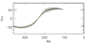
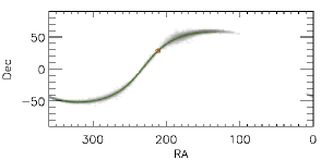
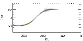
Figure 7: Left panels: All-sky view of the tidal tails in our simulations. The solid green line shows the orbit of NGC 5466, its position today is marked with a red circle. Right panels: Maximum surface density along the tail. The sky is cut into square degrees in right ascension and declination and for each degree in right ascension the maximum surface density of all declinations is given. From top to bottom we show the results of the DB, ML and ML with revised proper motion models.

In the top left panel of Fig. 6, we show the data on the tails of NGC 5466 reproduced from Belokurov et al. (2006a), who used neural networks are used to reconstruct the probability density distribution. The contours correspond to level curves of equal neural network output and therefore trace the star density. The tails are clearly visible once the extragalactic contaminants (predominantly galaxy clusters) have been eliminated. The tails extend $\sim 4^{\circ}$ on the sky, corresponding to $\sim 1$ kpc in projected length.

Table 1: Results of the suite of simulations investigating the relation between orbit and density of the tidal tails. The columns give the following numbers: the absolute value of the proper motion, the proper motion in $\alpha$ and $\delta$, the peri- and apogalacticon distances, the mean density of the tails, the maximum density in the tails, the extent of the tails, and the final mass of the cluster in units of the initial mass.

$\left|\mu\right|$	$\mu_{\alpha}\cos\delta$	$\mu_{\delta}$	$R_{\rm peri}$	$R_{\rm apo}$	$\Sigma_{\rm mean}$	$\Sigma_{\rm max}$	Extent	Final cluster
mas yr-1	mas yr-1	mas yr-1	kpc	kpc	M⊙ deg-2	M⊙ deg-2	deg	mass
4.40	-4.40	0.00	4.9	42.9	30.6	81.5	249	0.74
4.61	-4.60	0.30	5.7	50.8	26.7	60.5	244	0.79
4.72	-4.70	0.42	5.9	57.5	25.5	56.3	244	0.80
4.84	-4.80	0.60	6.4	61.5	23.4	72.6	239	0.83
5.06	-5.00	0.80	7.0	73.0	21.5	54.0	239	0.87
5.30	-5.20	1.00	7.4	88.1	19.1	47.0	230	0.89
5.60	-5.45	1.30	8.0	116.9	14.9	31.6	224	0.92

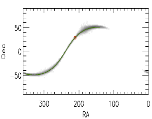
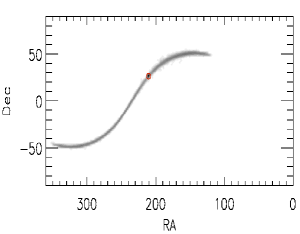
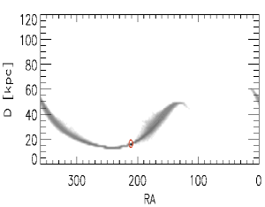
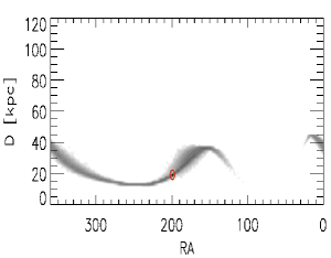
Figure 8: Simulations with different proper motions. The rows show from top to bottom: the projection of the tidal tails in $\alpha$ and $\delta$, the distance distribution of the tails vs. $\alpha$ and finally the surface density of the tails vs. $\alpha$. The columns show first the simulation with the smallest magnitude in proper motion, our best fitting model and finally the model with the highest magnitude of proper motion.

In the next two panels of Fig. 6, we show the projection on the sky of our models in the ML and DB potentials after $10$ Gyr of evolution. Both models show faint tidal tails, which match the general shape of the contours well. However, one important feature of the data is not reproduced – the leading and trailing tails are well-aligned with the proper motion vector. This contrasts with the data, in which the inner parts of the leading tails are slightly below the proper motion vector, whilst the inner parts of the trailing tails are slightly above. However, the observed proper motions are not well determined and have large error-bars, so one possibility is that the proper motion of NGC 5466 should be either larger in right ascension or smaller in declination than the values given in the literature (e.g. Dinescu et al., 1999) to match the observed misalignment. We confirm this result by running another simulation with slightly changed proper motions, namely

$$\mu_{\alpha}\cos\delta = -4.7\ {\rm mas\,yr}^{-1}$$

$$\mu_{\delta} = 0.42\ {\rm mas\,yr}^{-1}.$$ (11)

This orbit gives a perigalacticon of $5.9$ kpc and an apogalacticon of $57.5$ kpc. Although the change in proper motion does not make a significant difference to the mass-loss rate, as shown in the right panel of Fig. 5, it does improve the match with the location of the observed tidal streams much better, including the misalignment. In the lower right panels of Fig. 6, we see that the inner parts of the leading tails are now slightly below the old proper motion vector, whilst the inner parts of the trailing tails are now slightly above.

4.2 The Tail Densities and Extent

Fig. 7 shows all-sky views of the tidal tails, together with density profiles obtained by counting particles. The surface density of the tidal tails falls off along the innermost tails very steeply and stays at a very low density of $20$–$50$ M_⊙ deg^-2 throughout the tails. These low densities are very hard to detect, even in surveys like SDSS. Grillmair & Johnson (2006) found long, almost linear and very tenuous tidal extensions to NGC 5466 using a matched filter. Although these extensions are hard to see in the SDSS data, they do receive some support from the simulations presented here. The tails of our model with the revised proper motion extend over $\sim 100^{\circ}$ on the sky. Grillmair & Johnson (2006) claim that the average density of the tails is about $10$–$20$ stars deg^-2, which is also in good agreement with out estimate. Interestingly, at the point where Grillmair & Johnson (2006) start to loose track of the leading arm, our model is close to its apogalacticon and the tails are spread out much wider than is the case close to the cluster.

Although our simulation with the revised proper motion provides a good representation of the data, it is clearly not unique. In particular, it is interesting to understand the variety of tidal tail morphology for NGC 5466, especially as forthcoming deeper photometry will provide stronger constraints on the modelling. Accordingly, we perform a suite of Superbox simulations to investigate how the choice of proper motion influences the mass-loss and hence the properties of the tidal tails. As a constraint, we only used proper motions which are within the $1\sigma$ error range of the observed value (Dinescu et al., 1999) and also require that the orbital path near the cluster aligns with the tails found by Belokurov et al. (2006a), i.e., have the same projected orbital path as our refined set of proper motion. All-sky views of selected simulations are shown in Fig. 8 and show significant differences in the morphology and the properties of the tails. Table 1 gives the parameters and the results for the entire suite of simulations.

The number of degrees in right ascension over which the tail is detectable represents a measure for the length of the tails. The mean density of the tails is calculated in the following way. We examine one degree in right ascension $\alpha$ and search for the highest surface density in the tails for each degree in declination $\delta$. From these values, we compute the average surface density over the range of right ascension for which the tails are present. The maximum density given in the table is computed from the square degree of the tails with the highest surface density. Effects of varying distances are not taken into account. Table 1 shows clearly that the closer the orbit is to the Galactic centre the more severe is the mass-loss and the higher is the density in the tails.

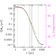
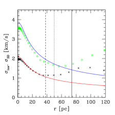
Figure 9: Left: Surface density distribution of our model of the NGC 5466 remnant. Left ordinate shows M_⊙ pc^-2, right ordinate shows mag arcsec^-2 using the M/L-ratio from literature of $1$. The inner part is still well fitted by the initial Plummer profile, while the outer parts are better fitted by a steeper power-law with index $-4.5$. The deviation is visible in the region from tidal radius at perigalacticon to tidal radius at apogalacticon. Vertical lines denote the tidal radius now (solid) and at the last perigalacticon (dashed), while dotted lines mark the grid boundaries with changes in resolution. Right: Velocity dispersion profile. Green open squares denote the 3D velocity dispersion measured in concentric shells around the cluster centre, crosses are the line-of-sight velocity dispersion measured in concentric rings around the cluster centre. Curves show the profile of the initial model. Vertical lines are as in the left panel.

4.3 The Remnant NGC 5466

Let us consider the internal properties of our remnant cluster in a representative simulation. We choose the one which uses the ML potential and the revised proper motions, shown in the lower right panels of Fig. 6. For this simulation, Fig. 9 shows the surface density and velocity dispersion profiles of the final cluster. Adopting the data from Harris (1996) (updated values from 2003), the cluster has a central surface brightness of $21.28$ mag arcsec^-2. This is in good agreement with our simulation, for which the central surface brightness is $20.6$ mag arcsec^-2, especially taking into account that our particle-mesh code neglects internal evolution, which would lead to higher densities in the core. Also, the half-light radius in our simulation is $10$ pc and corresponds well with the observed values of $10.4$ pc (Harris, 1996) and $13.1$ pc (Pryor et al., 1991). The actual tidal radius in our model is $75$ pc (using the Jacobi limit as given in Binney & Tremaine, 1987) and is less than the $158$ pc stated in Harris (1996) ($158$ pc) or $97$ pc in Lehmann & Scholz (1997), but only slightly larger than the radius of $61$ pc found by Pryor et al. (1991). Note that, observationally speaking, $r_{\rm tidal}$ is determined by fitting a King (1966) profile to the surface brightness distribution, which does not correspond exactly to the theoretical definition. According to our simulations, the tidal radius at the last perigalacticon was about $38$ pc.

While the surface density in the inner parts is not much affected by the mass-loss, the central velocity dispersion is reduced by approximately $10$ %. Also visible is a rise in the line-of-sight velocity dispersion in the outer parts, which starts already within the actual tidal radius. This is due to the fact that all line-of-sight measurements are contaminated by unbound stars streaming in front or behind the star cluster. While they do not affect the central values because of their low number, their effect is easily measurable in the outer parts where the densities of the bound stars are much lower.

5 Conclusions

We have presented numerical simulations of the formation and evolution of the tidal tails of the globular cluster NGC 5466. We used direct N-body codes to argue that the evolution of the cluster is dominated by external effects rather than internal relaxation, and then grid-based codes to trace the faint tidal tails. This novel, hybrid approach is well-suited to map out the detailed morphology of the low-density tails of NGC 5466.

Naively, we might expect that a low mass cluster with observed and very lengthy tails on a disc crossing orbit would not be able to survive for too much longer. However, simulations by Dehnen et al. (2004) have already shown that the disrupting globular cluster Pal 5 has survived for at least many Gyr in a tidally-dominated and out-of-equilibrium state, although Pal 5 probably will be destroyed at the next disc crossing. Here, we have demonstrated that a progenitor cluster of NGC 5466, which is quite similar to the present cluster, could survive substantially longer, for at least a few Hubble times, with its extensive but tenuous tidal tails gradually wrapping around the whole Galaxy.

The evolution of NGC 5466 is mainly driven by tidal shocks at each perigalacticon/disc crossing combination. Although not entirely negligible, internal effects (two-body relaxation and evaporation of stars driven by post-core collapsed processes (Lee & Goodman, 1995)) play a much less important role in the mass-loss. It is this property which allows us to study the tidal tails using grid-based codes rather than the more cumbersome direct N-body codes. If the observationally determined mass-to-light ratio of $\sim 1$ is correct, then the initial mass of NGC 5466 is $\sim 7\times 10^{4}$ M_⊙. By initial mass, we do not mean the embedded mass of the star cluster at its formation inside a gas-cloud. If the star formation efficiency is low, a star cluster can lose about $\sim 70$ per cent of its initial mass in stars when the gas gets blown out by high velocity winds or supernovae explosions. The rapid stellar evolution of high mass stars then adds another extreme mass-loss of $\sim 20$ per cent in the first few tens of Myr. After this initial phase of rapid evolution, the cluster reaches a quasi-equilibrium. This is the starting point of our simulations and therefore our initial mass refers to this point in time.

Our numerical simulations reproduce the observational results of both groups who have recently studied the tidal tails NGC 5466 with SDSS data. Mapping out the tails close to the globular cluster, Belokurov et al. (2006a) found that the leading tail emerges from the side pointing towards the Galactic Centre and returns to the orbital path from outside, while the trailing tail emerges from the side opposite to the Galactic Centre and returns to the orbital path from within. With our simulations, we showed that the proper motion of the globular cluster has to be smaller in declination and/or larger in right ascension than reported by Dinescu et al. (1999) to account for the position of the tidal tails. We propose a new set of proper motions, $\mu_{\alpha}\cos\delta=-4.7\ {\rm mas\,yr}^{-1}\mu_{\delta}=0.42\ {\rm mas\,yr}^{-1}$ for which the tail morphology is correctly reproduced. This differs from the observationally determined one by $-0.05$ and $-0.38$ mas yr^-1 respectively. These changes are within the error margins of the observed proper motion ($\pm 0.82$ mas yr^-1).

The surface density of the tidal tails falls off along the innermost tails very steeply and stays at a very low density of $20$–$50$ M_⊙ deg^-2 throughout the tails. These low densities are very hard to detect, even in surveys like SDSS. Grillmair & Johnson (2006) found long, almost linear and very tenuous tidal extensions to NGC 5466 using a matched filter approach. Their work is supported by the simulations in this paper, which show that the very long ($\mathrel{\hbox to0.0pt{\lower 3.0pt\hbox{$\mathchar 536\relax$}\hss}\raise 2.0pt\hbox{$\mathchar 318\relax$}}100^{\circ}$), faint tidal tails are expected. The tails in our simulation have roughly the same surface density as found by Grillmair & Johnson (2006).

In the future, deeper photometry, radial velocities and – thanks to the GAIA and SIM satellites – proper motions of individual stars in the tidal tails may become available. Mapping out the structure of the tails of globular clusters and dwarf galaxies will then provide powerful constraints on the Galactic potential. This work, together with the observational papers of Belokurov et al. (2006a) and Grillmair & Johnson (2006), has shown that NGC 5466 is a prime target for such studies of cold streams. Its tidal tails, though faint, are the longest so far claimed for any Milky Way globular cluster.

Acknowledgements: MF and VB are funded by PPARC. MIW acknowledges support from a Royal Society University Research Fellowship. We thank W. Dehnen for providing his Galactic potential code and R.Spurzem and H.M. Lee for useful comments. The direct N-body simulations were performed on the GRACE supercomputer at ARI-ZAH Heidelberg funded by Volkswagen Stiftung I/80 041-043 and the State of Baden-Württemberg, using GRAPE hardware.

References

- Aarseth (1999) Aarseth S.J., 1999, PASP, 111, 1333
- Aarseth et al. (1974) Aarseth S.J., Henon M., Wielen R., 1974, A&A, 37, 183
- Baumgardt & Makino (2003) Baumgardt H., Makino J., 2003, MNRAS, 340, 227
- Belokurov et al. (2006a) Belokurov V., Evans N.W., Irwin M.J., Hewett P.C., Wilkinson M.I., 2006a, ApJL, 637, L29
- Belokurov et al. (2006b) Belokurov, V., et al. 2006b, ApJ, 642, L137
- Belokurov et al. (2007) Belokurov, V., et al. 2007, ApJ, 658, 337
- Binney & Tremaine (1987) Binney J., Tremaine S., 1987, ’Galactic Dynamics’, Princeton University Press
- Dehnen & Binney (1998) Dehnen W., Binney J., 1998, MNRAS, 294, 429
- Dehnen et al. (2004) Dehnen W., Odenkirchen M., Grebel E. K., Rix H.-W. 2004, AJ, 127, 2753
- Dinescu et al. (1999) Dinescu D.I., Girard T.M., van Altena W.F., 1999, AJ, 117, 1792
- Fellhauer et al. (2000) Fellhauer M., Kroupa P., Baumgardt H., Bien R., Boily C.M., Spurzem R., Wassmer N., 2000, NewA, 5, 305
- Fellhauer et al. (2006) Fellhauer M., et al., 2006, ApJ, 651, 167
- Fellhauer et al. (2007) Fellhauer M., et al. 2007, MNRAS, 375, 1171
- Gnedin et al. (1999) Gnedin O.Y., Lee H.M., Ostriker J.P., 1999, ApJ, 522, 935
- Grillmair & Johnson (2006) Grillmair C.J., Johnson R., 2006, ApJL, 639, L17
- Harris (1996) Harris W.E., 1996, AJ, 112 1487
- Helmi (2004) Helmi A., 2004, ApJL, 610, L97
- Henon (1961) Henon M., 1961, AnAp, 24, 369
- Ibata et al. (1994) Ibata R.A., Gilmore G., Irwin M.J., 1994, Nature, 370, 194
- Johnston et al. (2005) Johnston K.V., Law D.R., Majewski S.R., 2005, ApJ, 619, 800
- King (1966) King I., 1966, AJ, 71, 61
- Lee & Ostriker (1987) Lee H.M., Ostriker J.P., 1987, ApJ, 322, 123
- Lee & Goodman (1995) Lee H.M., Goodman J., 1995, ApJ, 443, 109
- Lehmann & Scholz (1997) Lehmann I., Scholz R.-D., 1997, A&A, 320, 776
- Majewski et al. (2003) Majewski S.R., Skrutskie M.F., Weinberg M.D., Ostheimer J.C., 2003, ApJ, 599, 1082
- Meylan et al. (2001) Meylan G., Leon S., Combes F., 2001, in Deiters S., et al., (eds) ’Dynamics of Star Clusters and the Milky Way’, ASP Conference Series, 228, 53
- Odenkirchen et al. (2001) Odenkirchen M., et al. 2001, ApJ, 548, L165
- Odenkirchen et al. (2003) Odenkirchen M., et al. 2003, AJ, 126, 2385
- Plummer (1911) Plummer H.C., 1911, MNRAS, 71, 460
- Rockosi et al. (2002) Rockosi C., et al., 2002, AJ, 124, 349
- Pryor et al. (1991) Pryor C., McClure R.D., Fletcher J.M., Hesser J.E., 1991, AJ, 102, 1026
- York et al. (2000) York D.G., et al., 2000, AJ, 120, 1579
- Zucker et al. (2006) Zucker D.B., et al., 2006, ApJ, 650, L41