0706.2655 [hep-th]

Stability of string configurations dual
to quarkonium states in AdS/CFT

Spyros D. Avramis^1,2,x Konstadinos Sfetsos¹x andx Konstadinos Siampos¹

${}^{1}\!$ Department of Engineering Sciences, University of Patras,

26110 Patras, Greece

${}^{2}\!$ Department of Physics, National Technical University of Athens,

15773, Athens, Greece

avramis@mail.cern.ch,   sfetsos@upatras.gr,   ksiampos@upatras.gr

Abstract

We extend our earlier work, regarding the perturbative stability of string configurations used for computing the interaction potential of heavy quarks within the gauge/gravity correspondence, to cover a more general class of gravity duals. We provide results, mostly based on analytic methods and corroborated by numerical calculations, which apply to strings in a general class of backgrounds that encompass boosted, spinning and marginally-deformed D3-brane backgrounds. For the case of spinning branes we demonstrate in a few examples that perturbative stability of strings may require strong conditions complementing those following by thermodynamic stability of the dual field theories. For marginally-deformed backgrounds, we find that even in the conformal case stability requires an upper value for the imaginary part $\sigma$ of the deformation parameter, whereas in regions of the Coulomb branch where there exists linear confinement we find that there exist stable string configurations for certain ranges of values of the parameter $\sigma$. We finally discuss the case of open strings with fixed endpoints propagating in Rindler space, which turns out to have an exact classical-mechanical analog.

1 Introduction

The AdS/CFT correspondence [2] maps the computation of the Wilson-loop heavy quark-antiquark potential in the planar limit of ${\cal N}=4$ SYM to the classical minimal-surface problem of calculating the action of a string connecting the quark and antiquark on the boundary of ${\rm AdS}_{5}$ and extending into the radial direction [3]. However, when this method is applied to more general backgrounds [4, 5, 6, 7], one often encounters behaviors that are in sharp contrast with expectations based on the gauge-theory side [5]. A possible resolution could be that the parametric regions giving rise to these behaviors are perturbatively unstable and hence unphysical.

Let us summarize the basic relevant facts for the case of ${\cal N}=4$ SYM. In the standard conformal case, dual to a stack of D3-branes, this computation yields the expected Coulomb potential and all fluctuations about the classical string configuration are found to be stable [8, 9]. In extensions to the theory at finite temperature and at the Coulomb branch, dual to non-extremal and multicenter [10, 11, 12, 13] D3-branes respectively, one expects to find a screened Coulomb potential typical of thermal and Higgsed theories. However, one actually encounters situations where (i) the potential has a second branch of higher energy than the first, (ii) the potential exhibits a confining behavior at large distances, and (iii) the screening length is heavily dependent on the location of the probe string in the internal space. Although these types of behavior are quite counterintuitive, in a recent work [14] we established the reassuring result that the corresponding parametric regions represent string configurations that are perturbatively unstable, with the physical regions giving indeed the expected screened Coulomb potential. Our analysis, partly motivated by a mechanical analog, was based on the zero-mode behavior of the differential equations governing the small fluctuations about equilibrium and led to a formalism by means of which instabilities may be found by exact or approximate analytic methods. An important fact emerging from this analysis was the existence of instabilities due to fluctuations of non-cyclic angular coordinates, often appearing in cases where they are not a priori expected. In particular, these fluctuations cast the parametric region where confinement appears as unstable.

The analysis of [14] was restricted to diagonal metrics, where all fluctuations obey decoupled differential equations. However, there are physically interesting situations where the gravity duals where Wilson loops are evaluated contain non-diagonal metrics. A first class of such backgrounds are boosted (non-extremal) D3-brane backgrounds, used for evaluating the potential for a quark-antiquark pair moving with respect to the thermal medium [15, 16, 17, 18, 19, 20, 21]. For this case, the potential has a similar form to that in the zero-boost case, namely it is a double-branched function of the length with the lower branch corresponding to a screened Coulomb potential, but the screening length falls off as the velocity is increased. For this background, a numerical stability analysis has been presented in [22], indicating that the upper branch is perturbatively unstable. A second class of such backgrounds are spinning non-extremal D3-branes [10, 23, 24, 25], dual to ${\cal N}=4$ SYM at finite temperature and R-charge chemical potentials. The behavior is similar to that in the absence of chemical potentials, but the nontrivial dependence of the metrics on certain angles again calls for a stability analysis. Finally, a third class of such backgrounds are the Lunin–Maldacena deformations [26] (see also [27, 28]) of D3-brane backgrounds, dual to the Leigh–Strassler [29] deformations of ${\cal N}=4$ SYM which break supersymmetry down to ${\cal N}=1$. These backgrounds are characterized by the two real parameters $\gamma$ and $\sigma$. In the usual situation where the quark and antiquark are not taken to be separated in the internal space, only the $\sigma$–part of the deformation affects the potential (see [30] for investigations on the effect of $\gamma$–deformations), resulting in various behaviors ranging from the standard Coulomb behavior (for deformed ${\rm AdS}_{5}\times{\rm S}^{5}$) to complete screening and linear confinement [31, 32] (for the deformed multicenter D3-branes). To investigate the significance of these results, a stability analysis is again in order. We note that now the appearance of a confining potential is not in conflict with expectations from the gauge-theory side.

This article is organized as follows: In section 2, we give a brief review of the evaluation of Wilson loops in the backgrounds under consideration. In section 3, we analyze small fluctuations about the classical string configurations and we establish general results which allow us to determine the regions of instability using exact and approximate methods, generalizing the results of [14] to the non-diagonal case. In section 4, we apply these results to the gravity duals under consideration and we identify all unstable regions. In section 5, we summarize and conclude. In appendix A, we present the complete list of angular Schrödinger potentials for the backgrounds under consideration. In appendix B, we present the detailed solution of the equation for the angular fluctuations for a special case, in order to provide a consistency check of the numerical calculation employed in subsection 4.3.2. In appendix C, we apply our results to the problem of open strings in Rindler space, which turns out to have an exact classical-mechanical analog, namely the problem of the shape of a soap film stretched between two circular rings.

2 Wilson loops in AdS/CFT

In the framework of the AdS/CFT correspondence, the calculation of the Wilson-loop potential of a heavy quark-antiquark pair proceeds by considering a fundamental string whose endpoints lie on the two temporal sides of the Wilson loop, and which extends in the radial direction of the dual supergravity background so as to extremize its worldsheet area. This type of calculation was first considered in [3] for the conformal case and was extended to more general cases in [4, 5, 6, 16, 30]. Below, we give a brief review of this procedure, adapted to the case where the metric has off-diagonal elements in the directions transverse to the quark-antiquark axis and the $B$–field has nonzero components.

We consider a general background specified by a metric of the form

$$ds^{2}=G_{tt}dt^{2}+2G_{ti}dtdx_{i}+G_{ij}dx_{i}dx_{j}+G_{yy}dy^{2}+G_{uu}du^{2}+G_{ab}d\theta_{a}d\theta_{b}+\ldots\ ,$$ (2.1)

where, $y$ denotes the (cyclic) coordinate along the spatial side of the Wilson loop, $u$ denotes the radial direction extending from the UV at $u\to\infty$ down to the IR at some minimum value $u_{\rm min}$ determined by the geometry, $x_{i}$ stands for a generic cyclic coordinate, and $\theta_{a}$ stands for a generic non-cyclic coordinate. We also consider a $B$–field of the form

$$B_{2}=B_{ai}d\theta_{a}\wedge dx_{i}\ ,$$ (2.2)

as is the case with many interesting gravity duals of gauge theories [26, 32, 33, 34, 35]. For future convenience, we introduce the functions

$$g(u,\theta_{a})=-G_{tt}G_{uu}\ ,\qquad f_{y}(u,\theta_{a})=-G_{tt}G_{yy}\ ,$$

$$f_{ij}(u,\theta_{a})=G_{ti}G_{tj}-G_{tt}G_{ij}\ ,\quad f_{ab}(u,\theta_{a})=-G_{tt}G_{ab}\ ,\quad h(u,\theta_{a})=G_{yy}G_{uu}\ .$$ (2.3)

According to AdS/CFT, the potential energy of the quark-antiquark pair is given by

$$e^{-{\rm i}ET}=\langle W(C)\rangle=e^{{\rm i}S[C]}\ ,$$ (2.4)

where $S[C]$ is the action for a string propagating in the supergravity background whose endpoints trace the contour $C$. The latter is given by the sum of Nambu–Goto and Wess–Zumino terms,

$$S[C]=-{1\over 2\pi}\int d\tau d\sigma\left(\sqrt{-\det g_{\alpha\beta}}-{1\over 2}\epsilon^{\alpha\beta}b_{\alpha\beta}\right)\ ,$$ (2.5)

where $g_{\alpha\beta}$ and $b_{\alpha\beta}$ stand for the pullbacks

$$g_{\alpha\beta}=G_{\mu\nu}\partial_{\alpha}x^{\mu}\partial_{\beta}x^{\nu}\ ,\qquad b_{\alpha\beta}=B_{\mu\nu}\partial_{\alpha}x^{\mu}\partial_{\beta}x^{\nu}\ .$$ (2.6)

To proceed, we employ the gauge fixing

$$t=\tau\ ,\qquad u=\sigma\ ,$$ (2.7)

we assume translational invariance along $t$, and we consider the radial embedding

$$y=y(u)\ ,\qquad x_{i}={\rm const.}\ ,\qquad\theta_{a}=\theta_{a0}={\rm const.}\ ,$$ (2.8)

supplemented by the boundary condition

$$u\left(\pm{L\over 2}\right)=\infty\ ,$$ (2.9)

appropriate for a quark placed at $y=-L/2$ and an antiquark placed at $y=L/2$. In the ansatz (2.9), the constant values $\theta_{a0}$ of the non-cyclic coordinates $\theta_{a}$ must be consistent with the corresponding equation of motion. As we shall see later on, this requires that

$$\partial_{a}g(u,\theta_{a})|_{\theta_{a}=\theta_{a0}}=\partial_{a}f_{y}(u,\theta_{a})|_{\theta_{a}=\theta_{a0}}=0\ ;\qquad\partial_{a}\equiv{\partial\over\partial\theta_{a}}\ .$$ (2.10)

For the above ansatz, only the Nambu–Goto part of the action is nonzero, leading to

$$S=-{T\over 2\pi}\int du\sqrt{g(u)+f_{y}(u)y^{\prime 2}}\ ,$$ (2.11)

where $T$ denotes the temporal extent of the Wilson loop, the prime denotes a derivative with respect to $u$ while $g(u)\equiv g(u,\theta_{a0})$ and $f_{y}(u)\equiv f_{y}(u,\theta_{a0})$. Conservation of the momentum conjugate to $y$ implies that the classical solution $y_{\rm cl}(u)$ satisfies

$$y_{\rm cl}^{\prime}=\pm{\sqrt{f_{y0}F}\over f_{y}}\ ,$$ (2.12)

where $u_{0}$ is the value of $u$ at the turning point, $f_{y0}\equiv f_{y}(u_{0})$, the two signs correspond to the two branches around the turning point, and $F$ is defined as

$$F={gf_{y}\over f_{y}-f_{y0}}\ .$$ (2.13)

Integrating (2.13), we express the separation length as

$$L=2f_{y0}^{1/2}\int_{u_{0}}^{\infty}du{\sqrt{F}\over f_{y}}\ ,$$ (2.14)

while inserting (2.12) into (2.11) and using (2.4), we obtain the potential energy

$$E={1\over\pi}\int_{u_{0}}^{\infty}du\sqrt{F}-{1\over\pi}\int_{u_{\rm min}}^{\infty}du\sqrt{g}\ .$$ (2.15)

When the integrals (2.14) and (2.15) can be evaluated exactly and the first one can be inverted for $u_{0}$, these equations lead to an explicit expression for $E=E(L)$. However, in practice this cannot be done, except for a few simple cases, and Eqs. (2.14) and (2.15) are rather regarded as parametric equations for $L$ and $E$ with parameter $u_{0}$.

3 Stability analysis

We now turn to a stability analysis of these configurations just discussed, our goal being to identify all parametric regions which are unstable and for which information obtained using the gauge/gravity correspondence cannot be trusted. In this section we generalize the results of [14] to non-diagonal metrics of the form (2.1) and we establish a series of results which will ultimately allow us to identify the stable and unstable regions by a combination of exact and approximate analytic methods.

3.1 Small fluctuations

To investigate the stability of the string configurations of interest, we consider small fluctuations about the classical solutions discussed above. In particular, we will be interested in three types of fluctuations, namely (i) “transverse” fluctuations, referring to the cyclic coordinates $x_{i}$ transverse to the quark-antiquark axis, (ii) “longitudinal” fluctuations, referring to the cyclic coordinate $y$ along the quark-antiquark axis, and (iii) “angular” fluctuations, referring to the non-cyclic coordinates $\theta_{a}$. The above fluctuations may be parametrized by keeping the gauge choice (2.7) unperturbed and perturbing the embedding as

$$x_{i}=\delta x_{i}(t,u)\ ,\qquad y=y_{\rm cl}(u)+\delta y(t,u)\ ,\qquad\theta_{a}=\theta_{a0}+\delta\theta_{a}(t,u)\ .$$ (3.1)

Inserting this ansatz in the action (2.5) and expanding in powers of the fluctuations, we obtain the series

$$S=S_{0}+S_{1}+S_{2}+\ldots\ ,$$ (3.2)

with the subscripts corresponding to the respective powers of the fluctuations. The zeroth-order term gives just the classical action. The first-order contribution reads

$$\!\!\!\!S_{1}=-{1\over 2\pi}\int dtdu\left[\sqrt{f_{y0}}\ \delta y^{\prime}+\sqrt{{hF\over gf_{y}}}G_{ti}\delta\dot{x}_{i}+\left({1\over 2F^{1/2}}\partial_{a}g+{f_{y0}F^{1/2}\over 2f_{y}^{2}}\partial_{a}f_{y}\right)\delta\theta_{a}\right]\ ,$$ (3.3)

where $\partial_{a}g\equiv\partial_{a}g(u,\theta_{a})|_{\theta_{a}=\theta_{a0}}$ and $\partial_{a}f_{y}\equiv\partial_{a}f_{y}(u,\theta_{a})|_{\theta_{a}=\theta_{a0}}$. The first term is a surface contribution which is exactly cancelled by a similar term with the opposite sign corresponding to the contribution of the linear order action coming from the fluctuations of the lower string (cf. (2.12)), provided we keep the variations of both strings at $u=u_{0}$ equal. The second term is a total time derivative and hence is completely irrelevant. Finally, in the third term, the coefficient of $\delta\theta_{a}$ is just the equation of motion of $\theta_{a}$ and the requirement that it vanish leads indeed to the conditions (2.10). The second-order contribution is written as

$$\!\!\!\!\!\!\!\!\!\!\!\!S_{2} = -{1\over 2\pi}\int dtdu\biggl{[}f_{ij}\left({1\over 2F^{1/2}}\delta x_{i}^{\prime}\delta x_{j}^{\prime}-{hF^{1/2}\over 2gf_{y}}\delta\dot{x}_{i}\delta\dot{x}_{j}\right)+{gf_{y}\over 2F^{3/2}}\delta y^{\prime 2}-{h\over 2F^{1/2}}\delta\dot{y}^{2}$$

$$\qquad\qquad\quad\;-\sqrt{{hf_{y0}\over gf_{y}}}G_{ti}(\delta y^{\prime}\delta\dot{x}_{i}-\delta\dot{y}\delta x^{\prime}_{i})+B_{ai}(\delta\theta^{\prime}_{a}\delta\dot{x}_{i}-\delta\dot{\theta}_{a}\delta x^{\prime}_{i})$$

$$\qquad\qquad\quad\;+f_{ab}\left({1\over 2F^{1/2}}\delta\theta_{a}^{\prime}\delta\theta_{b}^{\prime}-{hF^{1/2}\over 2gf_{y}}\delta\dot{\theta}_{a}\delta\dot{\theta}_{b}\right)$$

$$\qquad\qquad\quad\;+\left({1\over 4F^{1/2}}\partial_{a}\partial_{b}g+{f_{y0}F^{1/2}\over 4f_{y}^{2}}\partial_{a}\partial_{b}f_{y}\right)\delta\theta_{a}\delta\theta_{b}\biggr{]}\ ,$$

again with all functions and their $\theta_{a}$–derivatives evaluated at $\theta_{a}=\theta_{a0}$. Writing down the equations of motion of the fluctuations and introducing a harmonic time dependence,

$$\delta x^{\mu}(t,u)=\delta x^{\mu}(u)e^{-{\rm i}\omega t}\ ,$$ (3.5)

we obtain the equations

$$\!\!\!\!\!\!\!\!\!\!\!\!\left[{d\over du}\left({f_{ij}\over F^{1/2}}{d\over du}\right)+\omega^{2}{hF^{1/2}f_{ij}\over gf_{y}}\right]\delta x_{j}-{\rm i}\omega\left[\partial_{u}\left(G_{ti}\sqrt{{hf_{y0}\over gf_{y}}}\right)\delta y-\partial_{u}B_{ai}\delta\theta_{a}\right]=0\ ,$$

$$\!\!\!\!\!\!\!\!\!\!\!\!\left[{d\over du}\left({gf_{y}\over F^{3/2}}{d\over du}\right)+\omega^{2}{h\over F^{1/2}}\right]\delta y+{\rm i}\omega\partial_{u}\left(G_{ti}\sqrt{{hf_{y0}\over gf_{y}}}\right)\delta x_{i}=0\ ,$$ (3.6)

$$\!\!\!\!\!\!\!\!\!\!\!\!\left[{d\over du}\left({f_{ab}\over F^{1/2}}{d\over du}\right)+\omega^{2}{hF^{1/2}f_{ab}\over gf_{y}}-\left({1\over 2F^{1/2}}\partial_{a}\partial_{b}g+{f_{y0}F^{1/2}\over 2f_{y}^{2}}\partial_{a}\partial_{b}f_{y}\right)\right]\delta\theta_{b}-{\rm i}\omega\partial_{u}B_{ai}\delta x_{i}=0\ .$$

for the transverse, longitudinal and angular fluctuations respectively. We see that the fluctuations generically couple to each other, satisfying a system of equations of the form

$$\left\{{d\over du}\left[\left(\begin{array}[]{ccc}\mathbf{p}_{x}&0&0\\ 0&p_{y}&0\\ 0&0&\mathbf{p}_{\theta}\\ \end{array}\right){d\over du}\right]+\left(\begin{array}[]{ccc}\omega^{2}\mathbf{q}_{x}&-{\rm i}\omega\boldsymbol{\gamma}&{\rm i}\omega\boldsymbol{\beta}^{T}\\ {\rm i}\omega\boldsymbol{\gamma}^{T}&\omega^{2}q_{y}&0\\ -{\rm i}\omega\boldsymbol{\beta}&0&\omega^{2}\mathbf{q}_{\theta}+\mathbf{r}_{\theta}\end{array}\right)\right\}\left(\begin{array}[]{c}\delta\mathbf{x}\\ \delta y\\ \delta\boldsymbol{\theta}\end{array}\right)=0\ ,$$ (3.7)

where the matrices $\mathbf{p}_{x}=(p_{ij})$, $\mathbf{p}_{\theta}=(p_{ab})$, $\mathbf{q}_{x}=(q_{ij})$, $\mathbf{q}_{\theta}=(q_{ab})$, $\mathbf{r}_{\theta}=(r_{ab})$, $\boldsymbol{\beta}=(\beta_{ai})$ and the column vector $\boldsymbol{\gamma}=(\gamma_{i})$ are read off from Eqs. (3.1). The problem is defined in the interval

$$u_{0}\leqslant u<\infty\ ,\qquad u_{0}>u_{\rm min}\ ,$$ (3.8)

and the boundary conditions for the fluctuations, determined by requiring that the string endpoints be held fixed and that the two parts of the string glue smoothly at $u=u_{0}$ read

$$\lim_{u\to\infty}\delta x_{i}(u)=0\ ,\qquad\lim_{u\to u_{0}^{+}}(u-u_{0})^{1/2}\delta x_{i}^{\prime}(u)=0\ ,$$

$$\lim_{u\to\infty}\delta y(u)=0\ ,\qquad\lim_{u\to u_{0}^{+}}\left[\delta y(u)+2(u-u_{0})\delta y^{\prime}(u)\right]=0\ ,$$ (3.9)

$$\lim_{u\to\infty}\delta\theta_{a}(u)=0\ ,\qquad\lim_{u\to u_{0}^{+}}(u-u_{0})^{1/2}\delta\theta_{a}^{\prime}(u)=0\ .$$

These boundary conditions follow from a straightforward extension of the proof given in [14] and is essentially based on the fact that $u=u_{0}$ and $u=\infty$ present regular singular points of the system (3.1). Therefore, our stability analysis has reduced to a coupled system of Sturm–Liouville equations, with our objective being to determine the range of values of $u_{0}$ for which the lowest eigenvalue becomes negative.

Ideally, one would like to solve the above Sturm–Liouville equations exactly, obtain the lowest eigenvalue $\omega_{0}^{2}$ in terms of the parameter $u_{0}$ and determine the regions where $\omega_{0}^{2}$ becomes negative. However, in most cases, this is impossible due to the complexity of the equations. On the other hand, it turns out that we can obtain useful information by studying a simpler problem, namely the zero-mode problem of the associated differential operators. Regarding the transverse and longitudinal fluctuations, we will use our Sturm–Liouville description to prove that transverse zero modes do not exist while longitudinal zero modes are in one-to-one correspondence with the critical points of the function $L(u_{0})$. For the angular fluctuations, we will employ an alternative Schrödinger description which allows us to identify angular zero modes using either exact or approximate methods.

3.2 Zero modes

To motivate the significance of zero modes for our stability analysis, we consider a Sturm–Liouville system of the form considered earlier on and we let $\omega_{n}^{2}(u_{0})$ be the corresponding eigenvalues. By standard results of Sturm–Liouville theory, these eigenvalues are real and strictly-ordered in the sense that $\omega_{0}^{2}(u_{0})<\omega_{1}^{2}(u_{0})<\ldots$, from which it also follows that different eigenvalues do not cross as we vary $u_{0}$. Furthermore, we know that, for sufficiently large values of $u_{0}$, all eigenvalues are positive. The above considerations imply that the first occurrence of instabilities will arise at a value of $u_{0}$ at which the lowest eigenvalue $\omega_{0}^{2}(u_{0})$ becomes negative. Therefore, a necessary condition for the appearance of instabilities is the existence of values $u_{0\rm c}^{(i)}$ of $u_{0}$ for which $\omega_{0}^{2}(u_{0})=0$. To verify that these zero modes really correspond to points where $\omega_{0}^{2}$ changes sign, we may solve the full Sturm–Liouville system near each critical point $u_{0\rm c}^{(i)}$, a task that may be accomplished using perturbative [14] or numerical methods. In fact, as we shall see later on, in all examples considered in this paper, a zero mode always signifies a change of sign of $\omega_{0}^{2}$ i.e. marks the boundary between a stable and an unstable region.

Restricting to zero modes simplifies our problem tremendously, as the three equations in (3.1) decouple, reducing to

$${d\over du}\left({f_{ij}\over F^{1/2}}{d\over du}\delta x_{j}\right)=0\ ,$$

$${d\over du}\left({gf_{y}\over F^{3/2}}{d\over du}\delta y\right)=0\ ,$$ (3.10)

$$\left[{d\over du}\left({f_{ab}\over F^{1/2}}{d\over du}\right)-\left({1\over 2F^{1/2}}\partial_{a}\partial_{b}g+{f_{y0}F^{1/2}\over 2f_{y}^{2}}\partial_{a}\partial_{b}f_{y}\right)\right]\delta\theta_{b}=0\ .$$

Using these simplified expressions, we will next prove that transverse zero modes do not exist and that longitudinal zero modes are in one-to-one correspondence with the critical points of the function $L(u_{0})$, and we will devise analytic methods for seeking angular zero modes. This is a fairly straightforward extension of the results of [14].

3.2.1 Transverse zero modes

We consider first the case of the transverse fluctuations. Using the definition of $F$ in (2.13), performing an integration by parts, and expanding about $u=u_{0}$, we write the general solution of the first of (3.2) as

$$\delta x_{i} = \int^{\infty}_{u}du\sqrt{gf_{y}\over f_{y}-f_{y0}}f^{-1}_{ij}c_{j}$$

$$= -2{\sqrt{gf_{y}}\over f_{y}^{\prime}}\sqrt{f_{y}-f_{y0}}f^{-1}_{ij}c_{j}-2\int_{u}^{\infty}du\sqrt{f_{y}-f_{y0}}\partial_{u}\left({\sqrt{gf_{y}}\over f_{y}^{\prime}}f^{-1}_{ij}\right)c_{j}$$

$$= -2\int_{u_{0}}^{\infty}du\sqrt{f_{y}-f_{y0}}\ \partial_{u}\left({\sqrt{gf_{y}}\over f_{y}^{\prime}}f^{-1}_{ij}\right)c_{j}-2\sqrt{g_{0}f_{y0}\over f^{\prime}_{y0}}f^{-1}_{ij0}c_{j}(u-u_{0})^{1/2}+{\cal O}(u-u_{0})\ ,$$

where the $c_{i}$ are constants. In order for this zero mode to exist, it must satisfy the first boundary condition in (3.1), which requires the coefficient of $(u-u_{0})^{1/2}$ to vanish. As the matrix $f^{-1}_{ij0}$ turns out not to admit any nontrivial null eigenvectors, this is only achieved when all $c_{i}=0$ i.e. for the trivial solution $\delta x_{i}=0$. Therefore, the transverse fluctuations do not lead to zero modes of the system (3.1).

3.2.2 Longitudinal zero modes

Turning to the longitudinal fluctuations, the fact that they decouple from the rest in the zero-mode analysis implies that the results of [14] for the diagonal case hold in our case as well. In particular, in [14] it was proven that the longitudinal zero-mode solution can be expressed in terms of the $u_{0}$–derivative of the length function as follows

$$\delta y\sim 2\sqrt{g_{0}f_{y0}\over f_{y0}^{\prime 3}}\ (u-u_{0})^{-1/2}+{\sqrt{f_{y0}}\over f_{y0}^{\prime}}L^{\prime}(u_{0})+{\cal O}\left((u-u_{0})^{1/2}\right)\ .$$ (3.12)

In order for this zero mode to exist, it must satisfy the second boundary condition in (3.1), which requires the constant term to vanish. Therefore, the solution exists only if

$$L^{\prime}(u_{0})=0\ ,$$ (3.13)

or, equivalently, if [14]

$$\int_{u_{0}}^{\infty}{du\over\sqrt{f_{y}-f_{y0}}}\ \partial_{u}\left(\sqrt{gf_{y}}\over f_{y}^{\prime}\right)=0\ ,$$ (3.14)

(a)	(b)	(c)	(d)

Figure 1: The four generic types of behavior of $L(u_{0})$ and $E(L)$ encountered in AdS/CFT calculations of Wilson loops, corresponding to (a) no critical points, Coulomb or screened Coulomb potential, (b) no critical points, Coulomb/confining potential, (c) one critical point, double-branched potential and (d) two critical points, multi-branched potential. The dashed parts of the curves indicate regions that are unstable under longitudinal perturbations.

which requires that the derivative term should change sign at least once as $u$ ranges in the interval $u\in[u_{0},\infty)$. Therefore, given the critical points of the length function, we may determine all values $u_{0\rm c}$ of $u_{0}$ where the system (3.1) has a zero mode. In view of our earlier remark that zero modes always signify a transition from a stable to an unstable region in our examples, the longitudinal instabilities for the various configurations of interest are as shown in Fig. 1. Additional instabilities may arise from angular perturbations, so that part(s) of the curves, stable under longitudinal perturbations only, might be actually unstable.

3.2.3 Angular zero modes

We finally consider angular fluctuations, which must be treated separately due to the fact that the non-cyclicity of the angular coordinates induces a “restoring force” term in the corresponding Sturm–Liouville equation, implying that we cannot write $\delta\theta_{a}$ in an explicit integral form, even in the zero-mode case. On the other hand, if we restrict to situations where the angular fluctuations are decoupled from the rest (which is indeed the case in most of our examples), the equation satisfied by each of the fluctuations can be easily brought to a Schrödinger form. This description allows us to determine the zero modes to quite high accuracy by using approximate methods. Following [14], we outline the procedure below.

Letting $\theta$ be any of the decoupled non-cyclic angular variables, the Sturm–Liouville equation for its fluctuations reads

$$\left[-{d\over du}\left(p_{\theta}{d\over du}\right)-r_{\theta}\right]\delta\theta=\omega^{2}q_{\theta}\delta\theta\ .$$ (3.15)

Employing the change of variables

$$x=\int_{u}^{\infty}du^{\prime}\sqrt{q_{\theta}\over p_{\theta}}\ \ ,\qquad\delta\theta=(p_{\theta}q_{\theta})^{-1/4}\Psi\ ,$$ (3.16)

we may transform Eq. (3.15) to a standard Schrödinger equation

$$\left[-{d^{2}\over dx^{2}}+V_{\theta}(x;u_{0})\right]\Psi(x)=\omega^{2}\Psi(x)\ ,$$ (3.17)

with the potential

$$V_{\theta}=-{r_{\theta}\over q_{\theta}}+{p_{\theta}^{1/4}\over q_{\theta}^{3/4}}{d\over du}\left[\left({p_{\theta}\over q_{\theta}}\right)^{1/2}{d\over du}(p_{\theta}q_{\theta})^{1/4}\right]=-{r_{\theta}\over q_{\theta}}+(p_{\theta}q_{\theta})^{-1/4}{d^{2}\over dx^{2}}(p_{\theta}q_{\theta})^{1/4}\ .$$ (3.18)

The problem is defined in the interval

$$0\leqslant x\leqslant x_{0}\ ,\qquad x_{0}=\int_{u_{0}}^{\infty}du\sqrt{q_{\theta}\over p_{\theta}}\ ,$$ (3.19)

which is finite, making the fact that the fluctuation spectrum is discrete manifest. The boundary conditions are simply

$$\Psi(0)=0\ ,\qquad\Psi^{\prime}(x_{0})=0\ .$$ (3.20)

Note that, in general, Eq. (3.16) does not lead to a closed expression for $u$ in terms of $x$ and therefore it is not always possible to write down the potential as an explicit function of $x$. In what follows, we will encounter cases where $V_{\theta}(x)$ can be determined exactly as well as cases where it may be adequately approximated by solvable potentials.

To develop our approximate methods, we first note that the behavior of the angular Schrödinger potential $V_{\theta}(u;u_{0})$ in the limits $u\to\infty$ and $u=u_{0}$ is given by

$$V_{\theta}(\infty,u_{0})=au^{2}+V_{\infty},$$ (3.21)

and

$$V_{\theta}(u_{0};u_{0})={1\over 8}{g_{0}f_{y0}f_{y0}^{\prime}\over h_{0}^{2}f_{\theta 0}^{2}}\ \partial_{u_{0}}\left(h_{0}f_{\theta 0}^{2}\over g_{0}f_{y0}\right)+{1\over 2}{g_{0}\over h_{0}f_{\theta 0}}\partial^{2}_{\theta}f_{y0}\equiv V_{0}\ ,$$ (3.22)

where $a$, $V_{\infty}$ and $V_{0}$ are finite quantities that depend on the parameter $u_{0}$. When $a\geqslant 0$, the potential expressed in terms of the variable $x$ rises from a minimum value to infinity in the finite interval $x\in[0,x_{0}]$, and hence it is reasonable to approximate it by an infinite well given by

$$V_{\rm approx}=\left\{\begin{array}[]{cl}\overline{V},&\quad 0\leqslant x\leqslant x_{0}\\ \infty\ ,&\quad{\rm otherwise}\end{array}\right\}\ ;\qquad\overline{V}\equiv\left\{\begin{array}[]{cl}{1\over 2}(V_{0}+V_{\infty}),&\quad a=0\\ V_{0},&\quad a\neq 0\end{array}\right\}\ .$$ (3.23)

With the boundary conditions (3.18) the energy levels read

$$\omega_{n}^{2}\ ={(2n+1)^{2}\pi^{2}\over 4[x_{0}(u_{0})]^{2}}+\overline{V}\ .$$ (3.24)

When $a=0$, this approximation is valid for both the ground state and the excited states. When $a>0$ however, the approximation is valid only for the ground state as excited states are affected by the details of the exact potential. In any case, we may determine the critical value $u_{0\rm c}$ by solving the equation $\omega^{2}_{0}(u_{0})=0$; clearly, a solution to this equation exists only if the average $\overline{V}$ is negative at least in a finite range of values of $u_{0}$. The infinite-well approximation just described is to be used for obtaining an indication for the existence of zero modes and for estimating $u_{0\rm c}$. In most cases, these estimates are quite close to the exact values, determined through numerical analysis.

4 Applications

Having developed the necessary formalism, we now turn to analyzing the stability properties of the string configurations of interest in backgrounds of boosted non-extremal D3-branes, spinning D3-branes and marginally-deformed D3-branes, all of which fall in the general category described by the metrics (2.1). For each case under consideration, we give the formulas for the length and the potential energy and we perform a stability analysis according to the guidelines of the previous section. Depending on the problem at hand, the regions of stability are determined by exact or approximate analytic methods, by the numerical solution of certain algebraic or transcendental equations, or by the numerical evaluation of certain integrals. In all cases, this represents a considerable improvement, both conceptual as well as practical, over the direct numerical solution of the differential equations governing the fluctuations.

4.1 Boosted non-extremal D3-branes

The first type of metrics we will consider are obtained by a boost of the metric for non-extremal D3-branes along one brane direction transverse to the quark-antiquark axis, say $x$. They are given by

$$ds^{2} = {u^{2}\over R^{2}}\left[-\left(1-{\gamma^{2}\mu^{4}\over u^{4}}\right)dt^{2}+2{\gamma^{2}v\mu^{4}\over u^{4}}dtdx+\left(1+{\gamma^{2}v^{2}\mu^{4}\over u^{4}}\right)dx^{2}+dy^{2}+dz^{2}\right]$$ (4.1)

$$+ R^{2}\left({u^{2}\over u^{4}-\mu^{4}}\ du^{2}+d\Omega_{5}^{2}\right)\ ,$$

where $v$ is the boost velocity and $\gamma=1/\sqrt{1-v^{2}}$. The metric has a horizon at

$$u_{H}=\mu\ ,$$ (4.2)

while there also exists a velocity-dependent radius $u_{\gamma}=\sqrt{\gamma}\mu\geqslant u_{H}$ beyond which the string cannot penetrate (see [15, 16, 17, 18, 20] for discussions). The Hawking temperature of the solution is given by $T=\mu/\pi R^{2}$. For the stability analysis for this metric, the “transverse” coordinates are $(x,z,\Omega_{5})$, with $x$ coupled to the longitudinal coordinate $y$, while no “angular” coordinates exist. This latter fact implies that the position of the string in the internal space can be arbitrary.

The calculation of the Wilson loops of section 2 for the above metric yields the potential for a quark and antiquark moving with velocity $v$ with respect to a thermal plasma at a temperature $T$ and may be used as a crude model for the study of meson dissociation in plasmas. Switching to dimensionless units by the change of variables

$$u\to\mu u\ ,\qquad u_{0}\to\mu u_{0}\ ,\qquad L\to{R^{2}\over\mu}L\ ,\qquad E\to{\mu\over\pi}E\ ,$$ (4.3)

we find that the length and the potential energy read [16, 20]

$$L(u_{0},\gamma)={2\sqrt{2}\pi^{3/2}\over\Gamma(1/4)^{2}}\ {\sqrt{u_{0}^{4}-\gamma^{2}}\over u_{0}^{3}}\ {}_{2}F\!_{1}\left({1\over 2},{3\over 4},{5\over 4};{1\over u_{0}^{4}}\right)\ ,$$ (4.4)

and

$$E(u_{0},\gamma)=-{\sqrt{2}\pi^{3/2}\over\Gamma(1/4)^{2}}\left[u_{0}\,{}_{2}F\!_{1}\left(-{1\over 4},{1\over 2},{1\over 4};{1\over u_{0}^{4}}\right)+{\gamma^{2}\over u_{0}^{3}}\ {}_{2}F\!_{1}\left({1\over 2},{3\over 4},{5\over 4};{1\over u_{0}^{4}}\right)\right]+1\ ,$$ (4.5)

where ${}_{2}F\!_{1}(a,b,c;x)$ is the standard hypergeometric function. The behavior of the length and the energy is as in Fig. 1c, with the maximal value of the length, $L_{\rm c}(u_{0},\gamma)$, being a decreasing function of the velocity and satisfying the approximate law $L_{\rm c}(u_{0},\gamma)\simeq\gamma^{-1/2}L_{\rm c}(u_{0},1)$ [16] indicating an enhancement of the dissociation rate of the quark-antiquark bound state with increasing velocity.

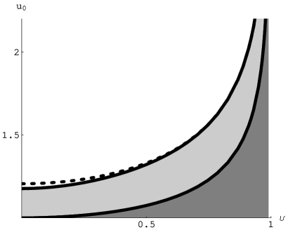
Figure 2: Stability diagram in the $(v,u_{0})$ plane for the case of the boosted non-extremal D3-brane background. The light-shaded region corresponds to instabilities under longitudinal perturbations and the dotted curve indicates our approximation (4.7) for $u_{0\rm c}(\gamma)$. The dark-shaded region corresponds to the values $u_{0}<\sqrt{\gamma}$ which are inaccessible to the string. The region $u_{0}<1$ beyond the horizon has been excluded from the diagram.

Turning to the stability analysis, our general results imply that the coupled system of the $(\delta y,\delta x)$ fluctuations has instabilities for $u_{0}<u_{0\rm c}(\gamma)$ where $u_{0\rm c}(\gamma)$ is the critical point of $L(u_{0},\gamma)$. The latter is determined by the solution of (3.13) which leads to the transcendental equation

$$5u_{0}^{4}(u_{0}^{4}-3\gamma^{2})\,{}_{2}F\!_{1}\left({1\over 2},{3\over 4},{5\over 4},{1\over u_{0}^{4}}\right)+6(u_{0}^{4}-\gamma^{2})\,{}_{2}F\!_{1}\left({3\over 2},{7\over 4},{9\over 4},{1\over u_{0}^{4}}\right)=0\ ,$$ (4.6)

which can be obtained numerically. For the physically interesting case $\gamma\gg 1$ (in which we also have $u_{0}\gg 1$) we can solve this equation perturbatively in $1/\gamma$ with the result

$$u_{0\rm c}(\gamma)=3^{1/4}\sqrt{\gamma}\left[1-{1\over 15\gamma^{2}}-{23\over 1350\gamma^{4}}+{\cal O}(\gamma^{-6})\right].$$ (4.7)

The results of the stability analysis just presented are summarized in the diagram of Fig. 2. Note that the estimate (4.7) for $u_{0\rm c}(\gamma)$ is remarkably close to the exact numerical result even for low velocities. Our results are in accordance with those of the numerical analysis presented in [22].

The above analysis may be extended to the case where the velocity and the axis of the quark-antiquark pair are not perpendicular but form an angle smaller than $\pi/2$. For such a case, we may modify our ansatz (2.8) to include a variable $x$ that has non-trivial dependence on $u$, while in the special case of motion parallel to the axis we may equivalently boost along the $y$ instead of the $x$ axis which would mean that the metric (2.1) would include an extra $G_{ty}$ term. Such string solutions were considered in [16, 18, 20, 21] and the behavior of the length and energy is again as in Fig. 1c. Hence we expect instabilities under longitudinal perturbations for $u_{0}<u_{0\rm c}(\gamma)$, a fact that we have actually verified by a small-fluctuation analysis which is however too lengthy to be included here.

4.2 Spinning D3-branes

We next consider the case of spinning (non-extremal) D3-branes, dual to ${\cal N}=4$ SYM theory at finite temperature and R-charge chemical potentials. These metrics were found in full generality in [10], based on previous results from [23], and their thermodynamical properties were examined in [25]. In the conventions of [24] which we here follow, the field-theory limit of these solutions is characterized by the non-extremality parameter $\mu$ and the angular momentum parameters $a_{i}$, $i=1,2,3$. Here, we will restrict to two special cases, corresponding to two equal nonzero angular momenta, $a_{2}=a_{3}=r_{0}$, and one nonzero angular momentum, $a_{1}=r_{0}$, to which we will apply our stability analysis.

4.2.1 Two equal nonzero angular momenta

For the case of two equal angular momenta, the metric reads

$$ds^{2} = H^{-1/2}\left[-\left(1-{\mu^{4}H\over R^{4}}\right)dt^{2}+dx^{2}+dy^{2}+dz^{2}\right]+H^{1/2}{u^{4}(u^{2}-r_{0}^{2}\cos^{2}\theta)\over(u^{4}-\mu^{4})(u^{2}-r_{0}^{2})}\ du^{2}$$

$$+ H^{1/2}\Big{[}(u^{2}-r_{0}^{2}\cos^{2}\theta)d\theta^{2}+u^{2}\cos^{2}\theta d\Omega_{3}^{2}+(u^{2}-r_{0}^{2})\sin^{2}\theta d\phi_{1}^{2}$$

$$\qquad\quad-\>\>2{\mu^{2}r_{0}\over R^{2}}\ dt\cos^{2}\theta(\sin^{2}\psi d\phi_{2}+\cos^{2}\psi d\phi_{3})\Big{]}\ ,$$

where

$$H={R^{4}\over u^{2}(u^{2}-r_{0}^{2}\cos^{2}\theta)}\$$ (4.9)

and $d\Omega^{2}_{3}=d\psi^{2}+\sin^{2}\psi d\phi_{2}^{2}+\cos^{2}\psi d\phi_{3}^{2}$. The metric has a horizon at

$$u_{H}=\mu\ ,$$ (4.10)

and considerations of thermodynamic stability restrict the ratio $\lambda\equiv\mu/r_{0}$ according to

$$\lambda\geqslant 1\hbox{ (CE)}\ ,\qquad\lambda\geqslant\sqrt{2}\hbox{ (GCE)}\ ,$$ (4.11)

where the two values refer to the canonical and grand-canonical ensembles respectively, with the former giving the lowest bounds in our examples. For the stability analysis for this metric, the “transverse” coordinates are $(x,z,\psi,\phi_{1,2,3})$, with $\phi_{2,3}$ coupled to the longitudinal coordinate $y$, and the only “angular” coordinate is $\theta$. The restriction (2.10) on the angular location $\theta_{0}$ of the string allows only trajectories with $\theta_{0}=0$ and $\theta_{0}=\pi/2$. To keep the discussion to a reasonable length, we will here restrict to the $\theta_{0}=\pi/2$ trajectories. For the trajectories with $\theta_{0}=0$, the longitudinal and angular fluctuations may be analyzed in the same way, using the Schrödinger potentials given in appendix A for the latter case.

To examine the Wilson-loop computation, we switch to dimensionless units by setting

$$u\to r_{0}u\ ,\qquad u_{0}\to r_{0}u_{0}\ ,\qquad L\to{R^{2}\over r_{0}}L\ ,\qquad E\to{r_{0}\over\pi}E\ .$$ (4.12)

Then, we find that the length and the potential energy are given by the expressions

$$L(u_{0},\lambda)=2\sqrt{u_{0}^{4}-\lambda^{4}}\int_{u_{0}}^{\infty}{du\,u\over\sqrt{(u^{2}-1)(u^{4}-u_{0}^{4})(u^{4}-\lambda^{4})}}\ ,$$ (4.13)

and

$$E(u_{0},\lambda)=\int_{u_{0}}^{\infty}du\,u\sqrt{u^{4}-\lambda^{4}\over(u^{2}-1)(u^{4}-u_{0}^{4})}-\int_{u_{H}}^{\infty}du{u\over\sqrt{u^{2}-1}}\ ,$$ (4.14)

which unfortunately cannot be evaluated in closed form. Their behavior is as in Fig. 1c.

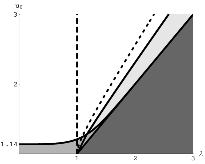
Figure 3: Stability diagram in the $(\lambda,u_{0})$ plane for the spinning D3-brane with two angular momenta and for the trajectory with $\theta_{0}=\pi/2$. The two light-shaded regions on the upper right-hand and lower left-hand sides correspond to instabilities under longitudinal and angular perturbations, respectively. The dark-shaded region corresponds to values of $u_{0}$ beyond the horizon. The region to the left of the vertical dashed line corresponds to the values $\lambda<1$ for which the background is thermodynamically unstable. The dotted line corresponds to the curve drawn using the approximation described below (4.15).

Turning to the stability analysis, our general results imply that the coupled system of the $(\delta y,\delta\phi_{2,3})$ fluctuations has instabilities for $u_{0}<u_{0\rm c}^{(y)}(\lambda)$ where $u_{0\rm c}^{(y)}(\lambda)$ is the critical point of $L(u_{0},\lambda)$. This value can be obtained by numerically solving the equation (3.14) which after some algebra takes the simple form

$$\int_{u_{0}}^{\infty}du{u^{6}-3\lambda^{4}u^{2}+2\lambda^{4}\over u^{3}\sqrt{(u^{2}-1)^{3}(u^{4}-u_{0}^{4})(u^{4}-\lambda^{4})}}=0\ .$$ (4.15)

In order for a solution to exist, the integrand must change sign at least once in the interval $u\in[u_{0},\infty)$. This requirement leads to the inequality $\lambda<u_{0}<\lambda\sqrt{2\cos(\phi/3)}$, where $\cos\phi=-1/\lambda^{2}$, hence $\phi\in[\pi/2,\pi]$. Taking the upper bound as an equality, i.e. $u_{0\rm c}^{(y)}(\lambda)=\lambda\sqrt{2\cos(\phi/3)}$, gives a quite good approximation to the exact numerical result, as one can see by inspection of Fig. 3.

Finally, for the angular fluctuations, the Schrödinger potential reads

$$V_{\theta}=-1\ ,$$ (4.16)

implying that the infinite-well approximation is exact in this case. Therefore, the critical value of $u_{0}$ beyond which instabilities occur are obtained by using Eq. 3.24, which is in fact exact in this case, with $\overline{V}=-1$ and solving the equation $\omega_{0}^{2}=0$. The resulting equation has the form

$$\int_{u_{0}}^{\infty}{du\,u^{3}\over\sqrt{(u^{2}-1)(u^{4}-u_{0}^{4})(u^{4}-\lambda^{4})}}={\pi\over 2}\ ,$$ (4.17)

and again can be solved numerically to give $u_{0\rm c}^{(\theta)}(\lambda)$. The results of this stability analysis are summarized in the diagram of Fig. 3.

4.2.2 One nonzero angular momentum

For the case of one angular momentum, the metric reads

$$ds^{2} = H^{-1/2}\left[-\left(1-{\mu^{4}H\over R^{4}}\right)dt^{2}+dx^{2}+dy^{2}+dz^{2}\right]+H^{1/2}{u^{2}(u^{2}+r_{0}^{2}\cos^{2}\theta)\over u^{4}+r_{0}^{2}u^{2}-\mu^{4}}\ du^{2}$$

$$+ H^{1/2}\Big{[}(u^{2}+r_{0}^{2}\cos^{2}\theta)d\theta^{2}+u^{2}\cos^{2}\theta d\Omega_{3}^{2}+(u^{2}+r_{0}^{2})\sin^{2}\theta d\phi_{1}^{2}$$

$$\qquad\quad-\>\>2{\mu^{2}r_{0}\over R^{2}}\sin^{2}\theta dtd\phi_{1}\Big{]}\ ,$$

where

$$H={R^{4}\over u^{2}(u^{2}+r_{0}^{2}\cos^{2}\theta)}\$$ (4.19)

and $d\Omega_{3}^{2}$ is as before. This metric has a horizon at

$$u_{H}^{2}={1\over 2}\left(-r_{0}^{2}+\sqrt{r_{0}^{4}+4\mu^{4}}\right)\ ,$$ (4.20)

and thermodynamic stability restricts $\lambda\equiv\mu/r_{0}$ to the range

$$\lambda\gtrsim 0.685\hbox{ (CE)}\ ,\qquad\lambda\gtrsim 0.93\hbox{ (GCE)}\ ,$$ (4.21)

for the canonical and grand-canonical ensembles respectively. For the stability analysis, the “transverse” and “angular” coordinates are as before, but now it is $\phi_{1}$ that couples to the longitudinal coordinate $y$. Again, the allowed trajectories have $\theta_{0}=0$ or $\theta_{0}=\pi/2$, and only the latter case will be considered here.

Using the same rescalings as before, we find that the expressions for the length and energy read

$$L(u_{0},\lambda)=2\sqrt{u_{0}^{4}-\lambda^{4}}\int_{u_{0}}^{\infty}{du\over\sqrt{(u^{4}-u_{0}^{4})(u^{4}+u^{2}-\lambda^{4})}}\ ,$$ (4.22)

and

$$E(u_{0},\lambda)=\int_{u_{0}}^{\infty}du{u^{4}-\lambda^{4}\over\sqrt{(u^{4}-u_{0}^{4})(u^{4}+u^{2}-\lambda^{4})}}\ -\int_{u_{H}}^{\infty}du\sqrt{{u^{4}-\lambda^{4}\over u^{4}+u^{2}-\lambda^{4}}}\ ,$$ (4.23)

which again cannot be evaluated in closed form. Their behavior is as in Fig. 1c.

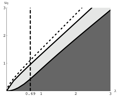
Figure 4: Stability diagram in the $(\lambda,u_{0})$ plane for the spinning D3-brane with one angular momentum and for the trajectory with $\theta_{0}=\pi/2$. The light-shaded region corresponds to instabilities under longitudinal perturbations. The dark-shaded region corresponds to values of $u_{0}$ beyond the horizon. The region to the left of the vertical dashed line corresponds to the values $\lambda\lesssim 0.685$ for which the background is thermodynamically unstable. The dotted line corresponds to the curve drawn using the approximation described below (4.24).

Turning to the stability analysis, the coupled system of the $(\delta y,\delta\phi_{1})$ fluctuations has instabilities for for $u_{0}<u_{0\rm c}(\lambda)$ where $u_{0\rm c}(\lambda)$ is the critical point of $L(u_{0},\lambda)$, obtained by numerically solving Eq. (3.14) which for our case reads

$$\int_{u_{0}}^{\infty}du{u^{8}-4\lambda^{4}u^{4}-4\lambda^{4}u^{2}+3\lambda^{8}\over u^{4}\sqrt{(u^{4}-u_{0}^{4})(u^{4}+u^{2}-\lambda^{4})^{3}}}=0\ .$$ (4.24)

This equation has a solution only if the integrand changes sign at least once in the interval $u\in[u_{0},\infty)$. This leads to the inequality $u_{H}<u_{0}<u_{\rm max}(\lambda)$ where $u_{\rm max}(\lambda)$ is the largest root of the numerator for which we will not present an explicit expression due to its complexity. As before, saturation of the upper bound gives a curve defined by $u_{0\rm c}(\lambda)=u_{\rm max}(\lambda)$ which gives a quite good approximation to the exact numerical result, as one can see by inspection of Fig. 4.

Finally, for the angular fluctuations, the Schrödinger potential reads

$$V_{\theta}=1\ ,$$ (4.25)

implying that no angular instabilities occur. The results of the stability analysis are summarized in the diagram of Fig. 4, which is qualitatively similar to Fig. 3 apart from the absence of angular instabilities.

4.3 Marginally-deformed D3-branes

We finally consider the Lunin–Maldacena deformations [26] of D3-brane solutions, dual to the Leigh–Strassler [29] marginal deformations of ${\cal N}=4$ SYM which break supersymmetry down to ${\cal N}=1$. These backgrounds are characterized by the complex parameter $\beta=\gamma+\tau\sigma$ (where $\tau$ is the Type IIB axion-dilaton and $\gamma$ and $\sigma$ are real parameters) which, on the gauge-theory side, represents the complex phase entering the Leigh–Strassler superpotential (where $\tau$ is the complexified gauge coupling). In particular, we will consider marginal deformations of the conformal ${\rm AdS}_{5}\times{\rm S}^{5}$ background [26] and of the multicenter backgrounds corresponding to D3-branes distributed on a sphere and on a disc [32].

4.3.1 The conformal case

Starting from the deformation of the conformal ${\rm AdS}_{5}\times{\rm S}^{5}$ background, we rescale the deformation parameters as $(\beta,\gamma,\sigma)\to{2\over R^{2}}(\beta,\gamma,g_{\rm s}\sigma)$ and we write the deformed metric as

$$ds^{2}={\cal H}^{1/2}\left[{u^{2}\over R^{2}}\left(-dt^{2}+dx^{2}+dy^{2}+dz^{2}\right)+R^{2}\left({du^{2}\over u^{2}}+d\Omega_{5,\beta}^{2}\right)\right]\ ,$$ (4.26)

where $d\Omega_{5,\beta}^{2}$ is the metric on the deformed ${\rm S}^{5}$, given by

$$d\Omega_{5,\beta}^{2} = d\theta^{2}+{\cal G}\sin^{2}\theta d\phi_{1}^{2}+\cos^{2}\theta[d\psi^{2}+{\cal G}(\sin^{2}\psi d\phi_{2}^{2}+\cos^{2}\psi d\phi_{3}^{2})]$$ (4.27)

$$+ {\cal G}|\beta|^{2}\cos^{4}\theta\sin^{2}\theta\sin^{2}2\psi\left(d\phi_{1}+d\phi_{2}+d\phi_{3}\right)^{2}\ ,$$

and the functions ${\cal G}$ and ${\cal H}$ are given by

$${\cal G}^{-1} = 1+4|\beta|^{2}\cos^{2}\theta(\sin^{2}\theta+\cos^{2}\theta\cos^{2}\psi\sin^{2}\psi)\ ,$$

$${\cal H} = 1+4\sigma^{2}\cos^{2}\theta(\sin^{2}\theta+\cos^{2}\theta\cos^{2}\psi\sin^{2}\psi)\ .$$ (4.28)

The solution also includes a nonzero $B$–field which, in the case when the deformation parameter $\gamma$ vanishes, is equal to

$$B_{2}={\sigma\over 2}\cos^{4}\theta\sin{2\psi}(d\phi_{1}+d\phi_{2}+d\phi_{3})\wedge d\psi\ ,$$ (4.29)

and hence is of the form (2.2). For the stability analysis for this and all subsequent metrics, the “transverse” coordinates are $(x,z,\phi_{1,2,3})$, with all of them being decoupled from the longitudinal coordinate $y$ but with the $\phi_{i}$ coupled to each other, while the “angular” coordinates are $(\theta,\psi)$, and are decoupled from each other. The restriction (2.10) on the angular location $(\theta_{0},\psi_{0})$ of the string allows only for the trajectories $(\theta_{0},\psi_{0})=(0,\pi/4)$, $(\theta_{0},\psi_{0})=(0,0\hbox{ or }\pi/2)$ (with both choices for $\psi_{0}$ leading to equivalent results), $(\theta_{0},\psi_{0})=(\pi/2,{\rm any})$, and $(\theta_{0},\psi_{0})=(\sin^{-1}(1/\sqrt{3}),\pi/4)$. All trajectories but the last will also be valid for the multicenter case with the branes distributed on the sphere and on a disc. We also note that for the trajectories with $\theta_{0}=\pi/2$ the variable $\psi$ becomes a completely decoupled “transverse” coordinate and hence its fluctuations are stable. Also, the presence of the nonzero $B$–field in (4.29) implies that, for the trajectories with $(\theta_{0},\psi_{0})=(0,\pi/4)$ and $(\theta_{0},\psi_{0})=(\sin^{-1}(1/\sqrt{3}),\pi/4)$, the angular fluctuation $\delta\psi$ and the transverse fluctuations $\delta\phi_{i}$ are actually coupled. However, the coupled terms are proportional to the eigenvalue $\omega$ and hence do not affect at all the results of our analysis which is based on the zero modes. For $(\theta_{0},\psi_{0})=(0,0\hbox{ or }\pi/2),(\pi/2,\text{any})$, $\delta\psi$ and $\delta\phi_{i}$ are decoupled.

For the present case, the potential energy $E$ can be calculated explicitly as a function of $L$ with the result

$$E(L)=k(\sigma)\left(-{4\pi^{2}R^{2}\over\Gamma(1/4)^{4}}{1\over L}\right)\ ,$$ (4.30)

where $k(\sigma)$ is an angle- and $\sigma$–dependent factor, given explicitly in the examples below, that becomes unity for $\sigma=0$. The factor in parentheses is the result of [3], giving the standard Coulomb behavior expected by conformal invariance. We note in passing that this factor is unaffected by turning on $\gamma$–deformations, unless the quarks are given a separation in the internal deformed sphere as well [30].

Regarding stability, the transverse/longitudinal fluctuations are obviously stable, while the Schrödinger potentials for the angular fluctuations all have the form

$$V_{\theta,\psi}=a_{\theta,\psi}(\sigma)u^{2}\ .$$ (4.31)

where $a_{\theta,\psi}(\sigma)$ are angle- and $\sigma$–dependent factors that can be read off the formulas of appendix A. The expression for the Schrödinger variable $x$ in terms of $u$ is

$$x={1\over u}\ {}_{2}F_{1}\left({1\over 4},{1\over 2},{5\over 4},{u_{0}^{4}\over u^{4}}\right)$$ (4.32)

and, accordingly, the value of the endpoint $x_{0}$ is

$$x_{0}={\Gamma(1/4)^{2}\over 4\sqrt{2\pi}}{1\over u_{0}}\ .$$ (4.33)

Instabilities may occur only when one of $a_{\theta,\psi}(\sigma)$ is negative. Although Eq. (4.32) cannot be inverted in terms of $u$ to allow for an analytic solution of the Schrödinger problem, we may obtain a lower bound for $\sigma$ above which instabilities definitely occur. We first note that the infinite-well approximation is not valid here, as the potential satisfies Eq. (3.21) with $a<0$. To obtain our bound, we consider the limit $u/u_{0}\gg 1$, where $x\simeq 1/u$ and $V_{\theta,\psi}\simeq a_{\theta,\psi}(\sigma)/x^{2}$. Then, standard arguments from quantum mechanics [37] show that for, $a_{\theta,\psi}(\sigma)<-{1\over 4}$, this potential supports an infinite tower of negative-energy states and the solution becomes unstable for all $u_{0}$. This gives the desired bound on $\sigma$. The results for the allowed trajectories are as follows:

$\bullet$ $(\theta_{0},\psi_{0})=(0,\pi/4)$. For this case we have

$$k(\sigma)=\sqrt{1+\sigma^{2}}\ ,\qquad a_{\theta}(\sigma)={2\sigma^{2}\over 1+\sigma^{2}}\ ,\qquad a_{\psi}(\sigma)=-{4\sigma^{2}\over 1+\sigma^{2}}\ .$$ (4.34)

Instabilities occur only from the $\delta\psi$ fluctuations for $\sigma>1/\sqrt{15}\simeq 0.258$. Since in the UV all marginally deformed backgrounds approach (4.26), (4.27), the above bound is universal as long as the corresponding trajectory remains valid. This is indeed the case for the sphere and disc brane distributions we consider.

$\bullet$ $(\theta_{0},\psi_{0})=(0,0\hbox{ or }\pi/2)$. Here, we have

$$k(\sigma)=1\ ,\qquad a_{\theta}(\sigma)=a_{\psi}(\sigma)=4\sigma^{2}\ ,$$ (4.35)

and no angular instabilities occur.

$\bullet$ $(\theta_{0},\psi_{0})=(\pi/2,{\rm any})$. Here, we have

$$k(\sigma)=1\ ,\qquad a_{\theta}(\sigma)=4\sigma^{2}\ ,$$ (4.36)

and again no angular instabilities occur.

$\bullet$ $(\theta_{0},\psi_{0})=(\sin^{-1}(1/\sqrt{3}),\pi/4)$. Here, we have

$$k(\sigma)=\sqrt{1+{4\sigma^{2}\over 3}}\ ,\qquad a_{\theta}(\sigma)=a_{\psi}(\sigma)=-{8\sigma^{2}\over 3+4\sigma^{2}}\ .$$ (4.37)

Instabilities occur from both $\delta\theta$ and $\delta\psi$ fluctuations for $\sigma>\sqrt{3/28}\simeq 0.327$. This bound does not survive in the multicenter cases we consider below since the corresponding trajectory is no longer valid.

Note that the existence of un upper bound for the deformation parameter $\sigma$ beyond which stability breaks down is reminiscent of an analogous fact for giant gravitons on the pp-wave limit of the deformed background (4.26), (4.27), which exist only for values of $\sigma<1/\sqrt{12}$. These giant graviton solutions can be thought of as integrated perturbations around their infinitesimal size. This implies that every order in the small size perturbative expansion of the giant graviton solution is unstable if the above bound is not respected. The different upper value for $\sigma$ in this case should be attributed to the fact that the probes in the giant graviton case refer to D3-branes and not to strings.

4.3.2 The sphere

We next consider the deformation of the background corresponding to D3-branes distributed on a sphere of radius $r_{0}$. Switching to dimensionless units by using Eq. (4.12), we write the deformed metric as [32]

$$\!\!\!\!\!\!\!\!\!\!\!\!\!\!ds^{2}={\cal H}^{1/2}\Biggl{\{}H^{-1/2}\left(-dt^{2}+dx^{2}+dy^{2}+dz^{2}\right)+H^{1/2}{u^{2}-r_{0}^{2}\cos^{2}\theta\over u^{2}-r_{0}^{2}}du^{2}$$

$$\!\!\!\!\!\!\!\!\!\!\!\!\!\!\ \qquad\qquad\quad+\>\>H^{1/2}\left[(u^{2}-r_{0}^{2}\cos^{2}\theta)d\theta^{2}+{\cal G}(u^{2}-r_{0}^{2})\sin^{2}\theta d\phi_{1}^{2}\right]$$

$$\!\!\!\!\!\!\!\!\!\!\!\!\!\!\ \qquad\qquad\quad+\>\>H^{1/2}u^{2}\cos^{2}\theta\left[d\psi^{2}+{\cal G}(\sin^{2}\psi d\phi_{2}^{2}+\cos^{2}\psi d\phi_{3}^{2})\right]$$

$$\!\!\!\!\!\!\!\!\!\!\!\!\!\!\ \qquad\qquad\quad+\>\>H^{1/2}{|\beta|^{2}{\cal G}u^{2}(u^{2}-r_{0}^{2})\cos^{4}\theta\sin^{2}\theta\sin^{2}2\psi\over u^{2}-r_{0}^{2}\cos^{2}\theta}\left(d\phi_{1}+d\phi_{2}+d\phi_{3}\right)^{2}\Biggr{\}}\ ,$$ (4.38)

with

$${\cal G}^{-1} = 1+4|\beta|^{2}\cos^{2}\theta\ {(u^{2}-r_{0}^{2})\sin^{2}\theta+u^{2}\cos^{2}\theta\cos^{2}\psi\sin^{2}\psi\over u^{2}-r_{0}^{2}\cos^{2}\theta}\ ,$$

$${\cal H} = 1+4\sigma^{2}\cos^{2}\theta\ {(u^{2}-r_{0}^{2})\sin^{2}\theta+u^{2}\cos^{2}\theta\cos^{2}\psi\sin^{2}\psi\over u^{2}-r_{0}^{2}\cos^{2}\theta}\ ,$$ (4.39)

and $H$ is given by (4.9). We also note that here there is a nonzero $B$–field which for $\gamma=0$ is proportional to the expression given in (4.29). Now, the restriction (2.10) on the $(\theta_{0},\psi_{0})$ of the string allows only for the first three trajectories considered earlier, namely $(\theta_{0},\psi_{0})=(0,\pi/4)$, $(\theta_{0},\psi_{0})=(0,0\hbox{ or }\pi/2)$ and $(\theta_{0},\psi_{0})=(\pi/2,{\rm any})$.

We next examine the potentials arising in each case in turn:

$\bullet$ $(\theta_{0},\psi_{0})=(0,\pi/4)$. The length and potential energy read (see sec. 6.2 of [32])

$$L(u_{0},\sigma)={2u_{0}\over\sqrt{(u_{0}^{2}-{1\over 1+\sigma^{2}})(2u_{0}^{2}-{1\over 1+\sigma^{2}})}}\left[{\bf\Pi}(a^{2},k)-{\bf K}(k)\right]\ ,$$ (4.40)

and

$$E(u_{0},\sigma)=\sqrt{1+\sigma^{2}}\left\{\sqrt{2u_{0}^{2}-{1\over 1+\sigma^{2}}}\left[a^{2}{\bf K}(k)-{\bf E}(k)\right]+{\bf E}(c)-{\sigma^{2}\over 1+\sigma^{2}}{\bf K}(c)\right\}\ ,$$ (4.41)

where

$$k=\sqrt{{u_{0}^{2}+{\sigma^{2}\over 1+\sigma^{2}}\over 2u_{0}^{2}-{1\over 1+\sigma^{2}}}}\ ,\qquad a=\sqrt{{u_{0}^{2}-{1\over 1+\sigma^{2}}\over 2u_{0}^{2}-{1\over 1+\sigma^{2}}}}\ ,\qquad c={1\over\sqrt{1+\sigma^{2}}}\ .$$ (4.42)

Note that these results are independent of the deformation parameter $\gamma$. The reason is that, as remarked also in the conformal case, we have not separated the quarks in the internal deformed-sphere space. Wilson-loop potentials where such a separation was considered, but with vanishing $\sigma$–deformation, were computed in [30].

For $\sigma=0$, the behavior of the length and energy is the same as for the undeformed case (Fig. 1c). As $\sigma$ is turned on, the length and energy curves are reminiscent of van der Waals isotherms for a statistical system with $u_{0}$, $L$ and $E$ corresponding to volume, pressure and Gibbs potential respectively (see e.g. [38]). In particular, there exists a critical value of $\sigma$, given by $\sigma_{\rm cr}^{(y)}\simeq 0.209$ (found analytically in [32]), below which the system behaves like the statistical system at $T<T_{\rm cr}$ (Fig. 1d) and above which the system behaves like the statistical system at $T>T_{\rm cr}$ (Fig. 1b). For nonzero $\sigma$, we have the usual Coulombic behavior for large $u_{0}$ (small $L$), while in the opposite limit, $u_{0}\to 1$, (large $L$), the asymptotics of (4.40) and (4.41) lead to the linear potential

$$E\simeq{\sigma\over 2}L\ .$$ (4.43)

To examine the significance of these results, it is crucial to examine the stability of the corresponding string configurations.

Our general results imply that the solution is stable under transverse perturbations. For the longitudinal fluctuations, the fact that $L(u_{0})$ has two extrema $u_{0\rm c}^{(l1)}(\sigma)$ and $u_{0\rm c}^{(l2)}(\sigma)$ for $0<\sigma<\sigma^{(y)}_{\rm cr}$ and no extrema for $\sigma>\sigma^{(y)}_{\rm cr}$ leads us to expect longitudinal instabilities in the region $u_{0\rm c}^{(l1)}(\sigma)<u_{0}<u_{0\rm c}^{(l2)}(\sigma)$ of $u_{0}$ (cf. Fig. 1d) in the first case, and no instabilities (cf. Fig. 1b) in the second case. To verify that the lowest eigenvalue $\omega_{0}^{2}$ does indeed change sign at these values, we performed a numerical analysis whose results are shown in Fig. 5b and indeed reproduce the expected behavior. Finally, for the angular fluctuations, the relevant Schrödinger potentials are given by the complicated expressions in Eqs. (A) of appendix A. Starting from $V_{\theta}$, we find that for $\sigma<0.71$ it is positive while for $\sigma>0.71$ it develops a negative part which means that it can in principle support a bound state of negative energy. The critical value $\sigma^{(\theta)}_{\rm cr}$ above which such states can exist is determined in the infinite-well approximation to be $\sigma^{(\theta)}_{\rm cr}\simeq 0.78$, which is quite close to the true value $\sigma^{(\theta)}_{\rm cr}\simeq 0.805$ determined by numerical analysis. As $\sigma$ increases beyond this value, the corresponding critical value $u_{0\rm c}^{(\theta)}$ approaches the value of 1.097 as $\sigma$ becomes very large. Turning to the $\delta\psi$ fluctuations, the same reasoning used in the deformation of the conformal background for the same trajectory carries over to the present case, implying that there exists a critical value $\sigma^{(\psi)}_{\rm cr}=1/\sqrt{15}$ (within our numerical limitations) above which there occur instabilities for all values of $u_{0}$. This value is presumably inherited by the conformal limit of the potential as analyzed in subsection 4.3.1. The above results are summarized in the stability diagram of Fig. 5.

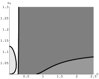
(a)	(b)	(c)

Figure 5: (a) Stability diagram in the $(\sigma,u_{0})$ plane for the deformed sphere and the trajectory with $(\theta_{0},\psi_{0})=(0,\pi/4)$. The three shaded regions correspond to instabilities due to longitudinal, $\delta\theta$ and $\delta\psi$ fluctuations (lightest to darkest). The origin $(0,1)$ actually belongs to the stable part of the diagram. Specifically, it is stable on its own right, but nowhere in its vicinity (for an analogous explicit example see sec. 5.4 of [14]). (b) Evolution of the lowest eigenvalue of the longitudinal fluctuations with $u_{0}$, plotted for $\sigma=0$, $0.15<\sigma^{(y)}_{\rm cr}$ and $0.5>\sigma^{(y)}_{\rm cr}$ (bottom to top). (c) Same for the angular $\delta\theta$ fluctuations, for $\sigma=0<\sigma^{(\theta)}_{\rm cr}$, $1>\sigma^{(\theta)}_{\rm cr}$ and $10\gg\sigma^{(\theta)}_{\rm cr}$ (top to bottom).

We also note that, in the limit $\sigma\gg 1$, the potential for the $\delta\theta$ fluctuations reads

$$V_{\theta}=2(u^{2}-2)+{\cal O}(\sigma^{-2})\ ,$$ (4.44)

and $x$ can be explicitly determined in terms of $u$ by (4.53). In this limit, the problem can be solved exactly (see appendix B), leading to the critical value $u_{0\rm c}^{(\theta)}\simeq 1.09737$, by mapping it to the well studied Lamé equation.

From the above we conclude that for a finite narrow range of values of the deformation parameter, namely for $0.209\simeq\sigma^{(y)}_{\rm cr}<\sigma<\sigma^{(\psi)}_{\rm cr}\simeq 0.258$ the linear confining behavior for large distances is stable, after which it is wiped out first by the instability of the $\delta\psi$ fluctuations and subsequently by the $\delta\theta$ ones. Moreover, even for smaller values of $\sigma$, namely for $0<\sigma<\sigma^{(y)}_{\rm cr}\simeq 0.209$, the confining behavior of potential is stable as we have discussed already.

$\bullet$ $(\theta_{0}=0,\psi_{0}=0\hbox{ or }\pi/2)$. The length and potential energy are the same as in the corresponding undeformed case, namely they are given by [5]

$$L(u_{0})={2u_{0}k^{\prime}\over u_{0}^{2}-1}\left[{\bf\Pi}(k^{\prime 2},k)-{\bf K}(k)\right]\ ,$$ (4.45)

and

$$E(u_{0})=\sqrt{2u_{0}^{2}-1}\left[k^{\prime 2}{\bf K}(k)-{\bf E}(k)\right]+1\ ,$$ (4.46)

where

$$k={u_{0}\over\sqrt{2u_{0}^{2}-1}}\ ,\qquad k^{\prime}=\sqrt{1-k^{2}}\ .$$ (4.47)

Their behavior is as in Fig. 1c.

By our general results, there exist longitudinal instabilities occurring for $u_{0}$ below the critical value for the undeformed case, namely $u_{0\rm c}\simeq 1.125$. For the angular $\delta\theta$ and $\delta\psi$ fluctuations, the Schrödinger potentials are given by (A.14) of appendix A and differ by the ones in the undeformed case by the positive-definite term $4\sigma^{2}u^{2}$, while the expression for the Schrödinger variable $x$ in terms of $u$ is the same as in the undeformed case. The above results imply that, since the $\delta\theta$ and $\delta\psi$ fluctuations are stable in the undeformed case, they are stable in the present case as well.

$\bullet$ $(\theta_{0},\psi_{0})=(\pi/2,{\rm any})$. In this case, the length and potential energy are again the same as in the undeformed case and are given by [5]

$$L(u_{0})={\sqrt{2}\over u_{0}}\left[{\bf\Pi}\left({1\over 2},k\right)-{\bf K}(k)\right]\ ,$$ (4.48)

and

$$E(u_{0})={u_{0}\over\sqrt{2}}\left[{\bf K}(k)-2{\bf E}(k)\right]\ .$$ (4.49)

where

$$k=\sqrt{{u_{0}^{2}+1\over 2u_{0}^{2}}}\ ,\qquad k^{\prime}=\sqrt{1-k^{2}}\ .$$ (4.50)

The behavior is as shown in Fig. 1b. For $u_{0}\gg 1$ (small $L$), the behavior is Coulombic, whereas in the opposite limit, $u_{0}\to 1$ (large $L$), the asymptotics of (4.48) and (4.49) lead to the linear potential

$$E\simeq{L\over 2}\ ,\qquad{\rm for}\quad L\gg 1\ .$$ (4.51)

In the undeformed case, the appearance of a linear confining potential is quite unexpected from the gauge-theory side and the paradox is resolved by the stability analysis of [14] which indicates that the configurations where this behavior appears are unstable under angular perturbations. However, for the deformed case, where ${\cal N}=4$ supersymmetry is broken to ${\cal N}=1$, the appearance of a confining potential is expected. Remarkably, this is confirmed by the stability analysis that follows:

We first note that the transverse and longitudinal fluctuations are manifestly stable, the latter fact following from the absence of extrema of $L(u_{0})$. For the angular fluctuations, the Schrödinger potential reads

$$V_{\theta}=-1+4\sigma^{2}(u^{2}-1)\ ,$$ (4.52)

whence we see that the effect of the deformation is to modify $V_{\theta}$ (which, for the undeformed case equals $-1$) by a positive-semidefinite term. It is quite intuitive that the addition of this term will tend to stabilize the angular fluctuations. To see how this occurs, we note that in the present case, the Schrödinger variable $x$ can be explicitly determined in terms of $u$ as

$$x=\sqrt{2k^{2}-1\over 2}\ {\bf F}(\nu,k)\ ,\qquad\nu=\sin^{-1}\sqrt{2u_{0}^{2}\over u^{2}+u_{0}^{2}}\ ,$$ (4.53)

where ${\bf F}(\nu,k)$ is the incomplete elliptic integral of the first kind and $k$ is the modulus defined in (4.50). Likewise, the endpoint $x_{0}$ is determined in terms of $u_{0}$ by

$$x_{0}=x(u_{0})=\sqrt{2k^{2}-1\over 2}\ {\bf K}(k)\ .$$ (4.54)

Then, as shown in detail in appendix B, the equation for the angular fluctuations takes the form (B.5) with $A$ and $h$ given by the second of (B). For general values of $\sigma$, this equation can be solved only numerically and the results are as shown in Fig. 6. We verify that the critical point $u_{0\rm c}$ below which instabilities occur is a decreasing function of $\sigma$ which implies that the region where confinement occurs is gradually stabilized as one increases $\sigma$.

We finally note that for the special values $4\sigma^{2}=n(n+1)$, where $n$ is a positive integer, (B.5) reduces to the Lamé equation and can be solved exactly, as done in appendix B for the particular case $n=1$. The resulting value of $u_{0\rm c}$, given in the second of (B), agrees with our numerical results.

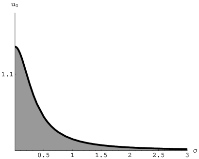
(a)	(b)

Figure 6: (a) Stability diagram in the $(\sigma,u_{0})$ plane for the deformed sphere and the trajectory with $(\theta_{0},\psi_{0})=(\pi/2,{\rm any})$. The shaded region corresponds to instabilities under angular perturbations. (b) Evolution of the lowest eigenvalue of the angular fluctuations with $u_{0}$, plotted for $\sigma=0$, $0.25$ and $0.5$ (bottom to top).

4.3.3 The disc

We finally consider the deformation of the background corresponding to D3-branes distributed on a disc of radius $r_{0}$, which is obtained from the deformed sphere background by the analytic continuation $r_{0}^{2}\to-r_{0}^{2}$. The possible trajectories are the same as for the sphere. We examine them in turn:

$\bullet$ $(\theta_{0},\psi_{0})=(0,\pi/4)$. The length and potential energy are given by (see sec. 6.2 of [32])

$$L(u_{0},\sigma)={2u_{0}\over\sqrt{(u_{0}^{2}+{1\over 1+\sigma^{2}})(2u_{0}^{2}+{1\over 1+\sigma^{2}})}}\left[{\bf\Pi}(a^{2},k)-{\bf K}(k)\right]\ ,$$ (4.55)

and

$$E(u_{0},\sigma)=\sqrt{1+\sigma^{2}}\left\{\sqrt{2u_{0}^{2}+{1\over 1+\sigma^{2}}}\left[a^{2}{\bf K}(k)-{\bf E}(k)\right]+{\bf E}(c)-{1\over 1+\sigma^{2}}{\bf K}(c)\right\}\ ,$$ (4.56)

where

$$k=\sqrt{{u_{0}^{2}-{\sigma^{2}\over 1+\sigma^{2}}\over 2u_{0}^{2}+{1\over 1+\sigma^{2}}}}\ ,\qquad a=\sqrt{{u_{0}^{2}+{1\over 1+\sigma^{2}}\over 2u_{0}^{2}+{1\over 1+\sigma^{2}}}}\ ,\qquad c={\sigma\over\sqrt{1+\sigma^{2}}}\ .$$ (4.57)

For $u_{0}\gg 1$ (small $L$) we recover the standard Coulombic behavior enhanced by the factor $\sqrt{1+\sigma^{2}}$, while for $u_{0}\to 0$ the asymptotics lead to the potential

$$E\simeq-{(\pi-L)^{2}\over 8{\bf E}({\rm i}\sigma)}\ ,$$ (4.58)

which shows that there is complete screening at the screening length

$$L_{\rm c}=\pi\ ,$$ (4.59)

that is invariant under $\sigma$–deformations.

Regarding stability, the solution is stable under transverse and longitudinal perturbations. Turning to angular fluctuations, the relevant Schrödinger potentials are given by the complicated expressions in Eqs. (A) of appendix A. Starting from the $\delta\theta$ fluctuations, we use the infinite-well approximation to find that the bottom of the well is raised with increasing $\sigma$ and that there is a critical value $\sigma^{(\theta)}_{\rm cr}>1/\sqrt{15}$ above which no instabilities exist. The existence of this critical value can be demonstrated by noting that for $\sigma\gg 1$, the potential takes the form

$$V_{\theta}\simeq 2(u^{2}+2)+{\cal O}(\sigma^{-2})\ .$$ (4.60)

This potential is positive and, using the techniques of appendix B, one can then show that perturbation theory holds about $\sigma\to\infty$. Thus, no instabilities occur in this limit. For the $\delta\psi$ fluctuations, the same arguments used for the deformed conformal background for the same trajectory show that there exists another critical value $\sigma^{(\psi)}_{\rm cr}=1/\sqrt{15}$ (again within numerical limitations and as before inherited by the conformal limit behavior of the solution) above which there occur instabilities for all values of $u_{0}$.

$\bullet$ $(\theta_{0},\psi_{0})=(0,0\hbox{ or }\pi/2)$. In this case we find that the classical solution is the same as in the undeformed disc at $\theta=0$ [5]

$$L(u_{0})={2u_{0}k^{\prime}\over u_{0}^{2}+1}\left[{\bf\Pi}(k^{\prime 2},k)-{\bf K}(k)\right]$$ (4.61)

and

$$E(u_{0})=\sqrt{2u_{0}^{2}+1}\left[k^{\prime 2}{\bf K}(k)-{\bf E}(k)\right]\ ,$$ (4.62)

where

$$k={u_{0}\over\sqrt{2u_{0}^{2}+1}}\ ,\qquad k^{\prime}=\sqrt{1-k^{2}}\ ,$$ (4.63)

Their behavior is as in Fig. 1a.

By our general results, the solution is stable under transverse and longitudinal perturbations. For the angular $\delta\theta$ and $\delta\psi$ fluctuations, the Schrödinger potentials are given by (A.17) of appendix A and again differ by the ones in the undeformed case by $4\sigma^{2}u^{2}$, while the expression for the Schrödinger variable $x$ in terms of $u$ is the same. For the $\delta\theta$ fluctuations, which have instabilities in the undeformed case, the extra term stabilizes the fluctuations and there exists critical value $\sigma^{(\theta)}_{\rm cr}$ above which there are no instabilities. Finally, the $\delta\psi$ fluctuations are stable in the undeformed case and hence are stable in the present case as well.

$\bullet$ $(\theta_{0},\psi_{0})=(\pi/2,{\rm any})$. The length and potential energy are given by [5]

$$L(u_{0})={2u_{<}^{2}\over\sqrt{u_{0}^{2}+u_{>}^{2}}}\left[{\bf\Pi}\left({u_{>}^{2}\over u_{0}^{2}+u_{>}^{2}},k\right)-{\bf K}(k)\right]\ ,$$ (4.64)

and

$$E(u_{0})={u_{0}^{2}\over\sqrt{u_{0}^{2}+u_{>}^{2}}}\ {\bf K}(k)-\sqrt{u_{0}^{2}+u_{>}^{2}}\ {\bf E}(k)+1\ ,$$ (4.65)

where now

$$k=\sqrt{{u_{>}^{2}-u_{<}^{2}\over u_{0}^{2}+u_{>}^{2}}}\ ,\qquad k^{\prime}=\sqrt{1-k^{2}}\$$ (4.66)

and $u_{>}$ ($u_{<}$) denotes the larger (smaller) between $u_{0}$ and $1$. Their behavior is as in Fig. 1a and, in particular, we have a screened Coulomb potential with screening length

$$L_{\rm c}={\pi\over 2}\ .$$ (4.67)

By familiar arguments, the solution is stable under transverse and longitudinal perturbations, whose behavior is insensitive to the deformation. Regarding the angular fluctuations, the Schrödinger potential (equal to $1$ in the undeformed case) now reads

$$V_{\theta}=1+4\sigma^{2}(u^{2}+1)\ ,$$ (4.68)

and hence the solution is still stable under angular perturbations.

5 Discussion and concluding remarks

In this paper, we completed the analysis of our earlier work [14] by developing a formalism for studying the perturbative stability of strings dual to quark-antiquark pairs in a wide class of backgrounds with non-diagonal metrics and possibly a $B$–field turned on. In particular, we derived a set of results by means of which the regions where instabilities occur can be determined by studying the zero modes of the differential equations governing the fluctuations. The simplifying fact making this extension possible is that, although the various fluctuations are generally coupled, their zero modes actually decouple so that the problem can be treated in an analytic manner similar to the diagonal case.

The methods developed here were applied to strings in boosted, spinning and marginally-deformed D3-brane backgrounds, dual to quarkonium states. For the case of boosted D3-branes, we easily recovered the result that instabilities appear for the energetically unfavored “long” strings stretching further into the radial direction. For the case of spinning branes, we found regions of instabilities due to both longitudinal and angular fluctuations. Finally, for the case of marginally-deformed D3-branes, we found that angular fluctuations tend to completely destabilize the classical solutions for large enough values of the deformation parameter $\sigma$, except for some special cases where the classical solutions are unaffected by the deformation and for which the deformation parameter $\sigma$ may actually have a stabilizing effect. In particular, we found parametric regions giving rise to a linear confining potential for which the dual string configurations are stable.

As the methods developed here are completely general, we expect that they are directly applicable to other backgrounds and, in particular to other gravity duals of gauge theories with reduced or no supersymmetry. As such backgrounds typically involve a non-trivial dependence on certain angular coordinates, it would be particularly interesting to determine the parametric regions for which quarkonium string configurations in these backgrounds are stable under angular perturbations. Extending our formalism to fluctuations of general brane probes should be also possible.

Acknowledgments

K. Sfetsos and K. Siampos acknowledge support provided through the European Community’s program “Constituents, Fundamental Forces and Symmetries of the Universe” with contract MRTN-CT-2004-005104, the INTAS contract 03-51-6346 “Strings, branes and higher-spin gauge fields”, the Greek Ministry of Education programs $\rm\Pi Y\Theta A\Gamma OPA\Sigma$ with contract 89194. K. Siampos also acknowledges support provided by the Greek State Scholarship Foundation (IKY).

Appendix A Angular Schrödinger potentials

Here we collect, for reference purposes, the Schrödinger potentials for angular fluctuations for all metrics and trajectories considered in the present paper as well as in [14].

Multicenter D3-branes

The only “angular” coordinate is $\theta$. The Schrödinger potentials for the various trajectories are given below.

$\bullet$ Sphere, $\theta_{0}=0$:

$$V_{\theta}(u;u_{0})={2u^{6}-u^{4}+[6u_{0}^{2}(u_{0}^{2}-1)-1]u^{2}-3u_{0}^{2}(u_{0}^{2}-1)\over 4u^{2}(u^{2}-1)^{2}}\ .$$ (A.1)

$\bullet$ Sphere, $\theta_{0}=\pi/2$:

$$V_{\theta}(u;u_{0})=-1\ .$$ (A.2)

$\bullet$ Disc, $\theta_{0}=0$:

$$V_{\theta}(u;u_{0})=-{2u^{6}+u^{4}+[6u_{0}^{2}(u_{0}^{2}+1)-1]u^{2}+3u_{0}^{2}(u_{0}^{2}+1)\over 4u^{2}(u^{2}+1)^{2}}\ .$$ (A.3)

$\bullet$ Disc, $\theta_{0}=\pi/2$.

$$V_{\theta}(u;u_{0})=1\ .$$ (A.4)

Spinning D3-branes

The only “angular” coordinate is $\theta$ as before. The Schrödinger potentials are given below.

$\bullet$ Two equal angular momenta, $\theta_{0}=0$:

$$\!\!\!\!\!\!\!\!V_{\theta}(u;u_{0},\lambda) = {1\over 4u^{6}(u^{2}-1)^{2}}\Bigl{\{}2u^{10}-u^{8}+\{6[u_{0}^{2}(u_{0}^{2}-1)+\lambda^{4}]-1\}u^{6}$$ (A.5)

$$- [3u_{0}^{2}(u_{0}^{2}-1)+11\lambda^{4}]u^{4}-5[2u_{0}^{2}(u_{0}^{2}-1)-1]\lambda^{4}u^{2}$$

$$+ 7u_{0}^{2}(u_{0}^{2}-1)\lambda^{4}\Bigr{\}}\ .$$

$\bullet$ Two equal angular momenta, $\theta_{0}=\pi/2$:

$$V_{\theta}(u;u_{0},\lambda)=-1\ .$$ (A.6)

$\bullet$ One angular momentum, $\theta_{0}=0$:

$$\!\!\!\!\!\!\!\!V_{\theta}(u;u_{0},\lambda) = -{1\over 4u^{4}(u^{2}+1)^{2}}\Bigl{\{}2u^{10}+3u^{8}+\{6[u_{0}^{2}(u_{0}^{2}+1)+\lambda^{4}]-1\}u^{6}$$ (A.7)

$$+ \{9[u_{0}^{2}(u_{0}^{2}+1)+\lambda^{4}]-1\}u^{4}+[(3-10\lambda^{4})u_{0}^{2}(u_{0}^{2}+1)+3\lambda^{4}]u^{2}$$

$$- 5u_{0}^{2}(u_{0}^{2}+1)\lambda^{4}\Bigr{\}}\ .$$

$\bullet$ One angular momentum, $\theta_{0}=\pi/2$:

$$V_{\theta}(u;u_{0},\lambda)=1\ .$$ (A.8)

Deformed D3-branes

Now, the “angular” coordinates are $\theta$ and $\psi$, with $\psi$ becoming irrelevant for the trajectories with $\theta_{0}=\pi/2$. The Schrödinger potentials are as follows.

$\bullet$ Conformal, $(\theta_{0},\psi_{0})=(0,\pi/4)$:

$$V_{\theta}(u;u_{0},\sigma)={2\sigma^{2}\over 1+\sigma^{2}}u^{2}\ ,\qquad V_{\psi}(u;u_{0},\sigma)=-{4\sigma^{2}\over 1+\sigma^{2}}u^{2}\ .$$ (A.9)

$\bullet$ Conformal, $(\theta_{0},\psi_{0})=(0,0\hbox{ or }\pi/2)$:

$$V_{\theta}(u;u_{0},\sigma)=V_{\psi}(u;u_{0},\sigma)=4\sigma^{2}u^{2}\ .$$ (A.10)

$\bullet$ Conformal, $(\theta_{0},\psi_{0})=(\pi/2,{\rm any})$:

$$V_{\theta}(u;u_{0},\sigma)=4\sigma^{2}u^{2}\ .$$ (A.11)

$\bullet$ Conformal, $(\theta_{0},\psi_{0})=(\sin^{-1}(1/\sqrt{3}),\pi/4)$:

$$V_{\theta}(u;u_{0},\sigma)=V_{\psi}(u;u_{0},\sigma)=-{8\sigma^{2}\over 3+4\sigma^{2}}u^{2}\ .$$ (A.12)

$\bullet$ Sphere, $(\theta_{0},\psi_{0})=(0,\pi/4)$:

$$V_{\theta}(u;u_{0},\sigma) = {1\over 4u^{2}[(1+\sigma^{2})u^{2}-1]^{3}}\Bigl{\{}8\sigma^{2}(1+\sigma^{2})u^{10}+2(1+\sigma^{2})(1-15\sigma^{2}+8\sigma^{4})u^{8}$$

$$- (3-41\sigma^{2}-36\sigma^{4})u^{6}+3\{2(1+\sigma^{2})u_{0}^{2}[(1+\sigma^{2})u_{0}^{2}-1]-7\sigma^{2}\}u^{4}$$

$$- \{(9+8\sigma^{2})[(1+\sigma^{2})u_{0}^{2}-1]-1\}u^{2}+3u_{0}^{2}[(1+\sigma^{2})u_{0}^{2}-1]\Bigr{\}}\ ,$$

$$V_{\psi}(u;u_{0},\sigma) = -{1\over 4u^{2}(u^{2}-1)[(1+\sigma^{2})u^{2}-1]^{3}}\Bigl{\{}16\sigma^{2}(1+\sigma^{2})u^{12}$$

$$- 2(1+\sigma^{2})(1+35\sigma^{2}+18\sigma^{4})u^{10}+(5+103\sigma^{2}+94\sigma^{4}+12\sigma^{6})u^{8}$$

$$+ \{6(1+\sigma^{2})(1+2\sigma^{2})u_{0}^{2}[(1+\sigma^{2})u_{0}^{2}-1]-3-54\sigma^{2}-20\sigma^{4}\}u^{6}$$

$$- \{(13+18\sigma^{2}+4\sigma^{4})u_{0}^{2}[(1+\sigma^{2})u_{0}^{2}-1]+1-7\sigma^{2}\}u^{4}$$

$$+ \{8u_{0}^{2}[(1+\sigma^{2})u_{0}^{2}-1]+1\}u^{2}-u_{0}^{2}[(1+\sigma^{2})u_{0}^{2}-1]\Bigr{\}}\ .$$

$\bullet$ Sphere, $(\theta_{0},\psi_{0})=(0,0\hbox{ or }\pi/2)$:

$$V_{\theta}(u;u_{0},\sigma)=V_{\theta}(u;u_{0})+4\sigma^{2}u^{2}\ ,\qquad V_{\psi}(u;u_{0},\sigma)=V_{\psi}(u;u_{0})+4\sigma^{2}u^{2}\ ,$$ (A.14)

where $V_{\theta}(u;u_{0})$ and $V_{\psi}(u;u_{0})$ are the potentials for the corresponding undeformed case, with the former given by (A.1) and the latter given by a function which, since the $\psi$ fluctuations in the multicenter case are stable, admits no negative-energy bound states. $\bullet$ Sphere, $(\theta_{0},\psi_{0})=(\pi/2,{\rm any})$:

$$V_{\theta}(u;u_{0},\sigma)=-1+4\sigma^{2}(u^{2}-1)\ .$$ (A.15)

$\bullet$ Disc, $(\theta_{0},\psi_{0})=(0,\pi/4)$:

$$V_{\theta}(u;u_{0},\sigma) = {1\over 4u^{2}[(1+\sigma^{2})u^{2}+1]^{3}}\Bigl{\{}8\sigma^{2}(1+\sigma^{2})u^{10}-2(1+\sigma^{2})(1-15\sigma^{2}-8\sigma^{4})u^{8}$$

$$- (3-41\sigma^{2}-36\sigma^{4})u^{6}-3\{2(1+\sigma^{2})u_{0}^{2}[(1+\sigma^{2})u_{0}^{2}+1]-7\sigma^{2}\}u^{4}$$

$$- \{(9+8\sigma^{2})[(1+\sigma^{2})u_{0}^{2}+1]-1\}u^{2}-3u_{0}^{2}[(1+\sigma^{2})u_{0}^{2}-1]\Bigr{\}}\ ,$$

$$V_{\psi}(u;u_{0},\sigma) = -{1\over 4u^{2}(u^{2}+1)[(1+\sigma^{2})u^{2}+1]^{3}}\Bigl{\{}16\sigma^{2}(1+\sigma^{2})u^{12}$$

$$+ 2(1+\sigma^{2})(1+35\sigma^{2}+18\sigma^{4})u^{10}+(5+103\sigma^{2}+94\sigma^{4}+12\sigma^{6})u^{8}$$

$$- \{6(1+\sigma^{2})(1+2\sigma^{2})u_{0}^{2}[(1+\sigma^{2})u_{0}^{2}+1]-3-54\sigma^{2}-20\sigma^{4}\}u^{6}$$

$$- \{(13+18\sigma^{2}+4\sigma^{4})u_{0}^{2}[(1+\sigma^{2})u_{0}^{2}+1]+1-7\sigma^{2}\}u^{4}$$

$$- \{8u_{0}^{2}[(1+\sigma^{2})u_{0}^{2}+1]+1\}u^{2}-u_{0}^{2}[(1+\sigma^{2})u_{0}^{2}+1]\Bigr{\}}\ .$$

$\bullet$ Disc, $(\theta_{0},\psi_{0})=(0,0\hbox{ or }\pi/2)$:

$$V_{\theta}(u;u_{0},\sigma)=V_{\theta}(u;u_{0})+4\sigma^{2}u^{2}\ ,\qquad V_{\psi}(u;u_{0},\sigma)=V_{\psi}(u;u_{0})+4\sigma^{2}u^{2}\ ,$$ (A.17)

where $V_{\theta}(u;u_{0})$ and $V_{\psi}(u;u_{0})$ are the potentials for the undeformed case, with the former given by (A.3) and the latter by a function admitting no negative-energy bound states.

$\bullet$ Disc, $(\theta_{0},\psi_{0})=(\pi/2,{\rm any})$:

$$V_{\theta}(u;u_{0},\sigma)=1+4\sigma^{2}(u^{2}+1)\ .$$ (A.18)

Appendix B Angular fluctuations and the Lamé equation

For the special cases of (i) the deformed sphere at $\theta_{0}=0$ in the limit $\sigma\gg 1$ and (ii) the deformed sphere at $\theta_{0}=\pi/2$ (for any $\sigma$), the Schrödinger equation for the angular fluctuations takes a relatively simple form that allows for explicit solutions. In both cases, the Schrödinger variable $x$ is given in closed form in terms of $u$ by Eq. (4.53), which can be inverted for $u$ to yield

$$u^{2}=2u_{0}^{2}\left({1\over{\rm sn}^{2}(\sqrt{2}u_{0}x,k)}-{1\over 2}\right)=2u_{0}^{2}\left(\wp(\sqrt{2}u_{0}x)+{1\over 6u_{0}^{2}}\right)\ ,$$ (B.1)

where ${\rm sn}(z,k)$ is the elliptic Jacobi function and $\wp(z)\equiv\wp(z\,|\,\omega_{1},\omega_{2})\equiv\wp(z,g_{2},g_{3})$ is the Weierstrass p-function, specified by the half-periods

$$\omega_{1}={\bf K}(k)\ ,\qquad\omega_{2}={\rm i}{\bf K}(k^{\prime})\ ,\qquad k^{2}={1+u_{0}^{2}\over 2u_{0}^{2}}\ ,$$ (B.2)

or, equivalently, by the elliptic invariants

$$g_{2}=-4(e_{1}e_{2}+e_{2}e_{3}+e_{3}e_{1})\ ,\qquad g_{3}=4e_{1}e_{2}e_{3}\ ,$$ (B.3)

with the $e_{i}$ given by

$$e_{1}={3u_{0}^{2}-1\over 6u_{0}^{2}}\ ,\qquad e_{2}={1\over 3u_{0}^{2}}\ ,\qquad e_{3}=-{3u_{0}^{2}+1\over 6u_{0}^{2}}\ ,$$ (B.4)

and satisfying $e_{1}+e_{2}+e_{3}=0$. Substituting (B.1) into (4.44) and (4.52) to obtain explicit expressions for the potentials in terms of $x$, and making a further change of variables to $z=\sqrt{2}u_{0}x$, we arrive at the following equation

$$\left\{-{d^{2}\over dz^{2}}+\left[A\wp(z)+h\right]\right\}\Psi(z)={\omega^{2}\over 2u_{0}^{2}}\Psi(z)\ ,\qquad 0\leqslant z\leqslant\omega_{1}\ ,$$ (B.5)

subject to the boundary conditions

$$\Psi(0)=0\ ,\qquad\Psi^{\prime}(\omega_{1})=0\ ,$$ (B.6)

and to the requirement that $\Psi(z)$ be real. Here, $A$ and $h$ stand for the constants

(i) $$: \>A=2\phantom{\sigma^{2}}\ ,\qquad h=-{5\over 3u_{0}^{2}}\ ,$$

(ii) $$: \>A=4\sigma^{2}\ ,\qquad h=-{3+4\sigma^{2}\over 6u_{0}^{2}}\ .$$ (B.7)

In the special cases where $A=n(n+1)$ (with $n$ being a positive integer) Eq. (B.5) is just the Lamé equation, whose exact solutions are well-known (see e.g. [39]). Although the construction of the specific solutions satisfying the boundary conditions (B.6) is rather cumbersome, it is instructive to consider the simplest possible case, $n=1$, as a consistency check of our numerics. For this case, the zero-mode equation simplifies to

$$\left\{-{d^{2}\over dz^{2}}+\left[2\wp(z)+h\right]\right\}\Psi(z)=0\ ,\qquad 0\leqslant z\leqslant\omega_{1}\ .$$ (B.8)

For the analysis that follows, it is convenient to define the quantities

$$a\equiv\wp^{-1}(h)\ ,\qquad\omega_{3}\equiv\omega_{1}+\omega_{2}\ .$$ (B.9)

When $a\neq\omega_{i}$, $i=1,2,3$, the equation (B.8) possesses the linearly-independent solutions

$$\Psi_{\pm}(z)=\exp\left[\mp z\upzeta(a)\right]{\upsigma(z\pm a)\over\upsigma(z)}\ ,$$ (B.10)

where $\upzeta(z)\equiv\upzeta(z\,|\,\omega_{1},\omega_{2})$ and $\upsigma(z)\equiv\upsigma(z\,|\,\omega_{1},\omega_{2})$ are the Weierstrass zeta and sigma functions.When $a=\omega_{i}$, the linearly-independent solutions are instead

$$\Psi_{i,1}(z)=\exp\left[-z\upzeta(\omega_{i})\right]{\upsigma(z+\omega_{i})\over\upsigma(z)}\ ,\qquad\Psi_{i,2}(z)=\left[\upzeta(z+\omega_{i})+ze_{i}\right]\Psi_{i,1}(z)\ .$$ (B.11)

For these two cases, the general solution reads $\Psi(z)=C_{+}\Psi_{+}(z)+C_{-}\Psi_{-}(z)$ and $\Psi(z)=C_{i,1}\Psi_{i,1}(z)+C_{i,2}\Psi_{i,2}(z)$ respectively. Imposing the condition $\Psi(0)=0$, we obtain $C_{+}=C_{-}$ and $C_{i,1}=-\upzeta(\omega_{i})C_{i,2}$ respectively, while using the reality condition for $\Psi(z)$ we find that $a$ must be real. For the case $a\neq\omega_{i}$, the condition $\Psi^{\prime}(\omega_{1})=0$ leads to the equation

$$\left\{\upsigma(\omega_{1}-a)\left[\upzeta(a)-\upzeta(\omega_{1})+\upzeta(\omega_{1}-a)\right]\right\}\left\{\exp\left[2\left(a\upzeta(\omega_{1})-\omega_{1}\upzeta(a)\right)\right]-1\right\}=0\ ,$$ (B.12)

which is to be solved for $a$ in the square $\{0\leqslant{\rm Re}\,a<2\omega_{1}\ ,\,0\leqslant{\rm Im}\,a<2|\omega_{2}|\}$ in the complex plane, due to the periodicity of the Weierstrass functions under $a\to a+2m\omega_{1}+2n\omega_{2}$. The trivial zeros of (B.12) occur at the points $a=\omega_{i}$, $i=1,2,3$ where either the first or the second factor in curly brackets vanishes. However, for these points, we actually have to use the second set of linearly-independent solutions (B.11). Doing so, we find that the values $a=\omega_{2,3}$ are not allowed due to the reality condition, while for the value $a=\omega_{1}$ the boundary condition $\Psi^{\prime}(\omega_{1})=0$ leads to the equation $3\upzeta(\omega_{1})=e_{1}\omega_{1}$, which has no solution. Nontrivial roots of Eq. (B.12) can only arise from the second factor in curly brackets, i.e. they are given by the solutions of the equation

$$a\upzeta(\omega_{1})=\omega_{1}\upzeta(a)\ ,$$ (B.13)

subject to the condition $a\neq\omega_{1}$. Using Eqs. (B), (B.2) and (B.9), we can express this as a transcendental equation for $u_{0\rm c}$, whose solutions for the two cases of interest are

(i) $$: \>u_{0\rm c}\simeq 1.09737\ ,\qquad L_{\rm c}=1.9312\ ,$$

(ii) $$: \>u_{0\rm c}\simeq 1.02676\ ,\qquad L_{\rm c}=2.92397\ ,\quad\hbox{for $4\sigma^{2}=2$}\ .$$ (B.14)

Both results are in precise agreement with our numerical analysis.

Appendix C Soap films and strings in Rindler space

An example of the calculations considered here and in [14] has been presented recently in [40] and refers to open strings ending on branes in Rindler space and their stability properties. As is well-known, Rindler space is (a portion of) flat Minkowski space, expressed in coordinates adapted to an observer at constant acceleration. Such an observer experiences the Unruh effect, perceiving the inertial vacuum as a state populated by a thermal distribution of particles at a temperature $T=\kappa/2\pi$, where $\kappa$ is the surface gravity. It is then natural to expect that an open string with fixed endpoints propagating in Rindler space will have similar properties as one propagating in a black-hole background and, in particular, will exhibit a phase structure of the type shown in Fig. 1c. In this appendix we prove the amusing fact that this problem is exactly equivalent to the classical-mechanical problem of the shape of a soap film suspended between two circular rings.

The metric for Rindler space has the form

$$ds^{2}=-\kappa^{2}u^{2}dt^{2}+dy^{2}+du^{2}+\ldots\ ,$$ (C.1)

where $u$ is the radial direction with the Rindler horizon corresponding to $u=0$ and $y$ is a generic spatial direction. The string configuration of interest corresponds to an open string with its two endpoints located at the same radius $u=\Lambda$ and separated by a distance $L$ along the $y$ direction. It is obvious that the formalism of section 2 readily applies to this setup. Passing to convenient dimensionless units through the rescalings

$$u\to\Lambda u\ ,\qquad u_{0}\to\Lambda u_{0}\ ,\qquad L\to\Lambda L\ ,\qquad E\to{\kappa\Lambda^{2}\over 4\pi^{2}}E\ ,$$ (C.2)

inserting the metric components of (C.1) in (2.12), and integrating from $u_{0}$ to $\Lambda$, we find that the classical solution is the catenary curve of Leibniz, Huygens and Bernoulli,

$$u=u_{0}\cosh{y\over u_{0}}\ ,$$ (C.3)

which is a slice of Euler’s catenoid. The integration constant $u_{0}$ and the energy of the string are determined by Eqs. (2.14) and (2.15) (without the subtraction term) which for our case read

$$L=2u_{0}\int_{u_{0}}^{1}{du\over\sqrt{u^{2}-u_{0}^{2}}}=2u_{0}\cosh^{-1}{1\over u_{0}}\ ,$$ (C.4)

and

$$E=4\pi\int_{u_{0}}^{1}{du\,u^{2}\over\sqrt{u^{2}-u_{0}^{2}}}=2\pi\left(\sqrt{1-u_{0}^{2}}+u_{0}^{2}\cosh^{-1}{1\over u_{0}}\right)\ ,$$ (C.5)

respectively. Eqs. (C.3)–(C.5) are exactly the same formulas appearing in Plateau’s problem for a thin soap film of mass density $1$ and surface tension ${1\over 2}$ stretched between two coaxial rings of radius $1$ that are separated by a distance $L$, with $u_{0}$ being the minimal radius reached by the film (see Eqs. (A.4)–(A.5) in appendix A of [14]), and thus the properties of the solutions (see e.g. [41]) are the same. Namely, there exists a critical value $u_{0\rm c}$ of $u_{0}$ and a corresponding value $L_{\rm c}$ of $L$ at which $L^{\prime}(u_{0})=0$, i.e.

$$\sqrt{1-u_{0}^{2}}\cosh^{-1}{1\over u_{0}}=1\ .$$ (C.6)

Solving this equation, we find $u_{0{\rm c}}\simeq 0.552$, whence $L_{\rm c}\simeq 1.325$ (to compare with the results of [40], set $u_{0\rm}\to L/h$). For separations $L<L_{\rm c}$, there is a “short” string (dual to the shallow catenoid), a “long” string of higher energy (dual to the deep catenoid), and a configuration of two straight strings (dual to the Goldschmidt solution). For separations $L>L_{\rm c}$, only the last configuration is possible.

Regarding stability, the only relevant fluctuations are the longitudinal fluctuations along $y$. By the results of section 2, instabilities occur for $u_{0}$ below the critical value where $L^{\prime}(u_{0})=0$ i.e. for $u_{0}<u_{0\rm c}$. This can be verified directly by noting that the longitudinal Sturm–Liouville equation has the form

$$(u^{2}-u_{0}^{2})\delta y^{\prime\prime}(u)+{u^{2}+2u_{0}^{2}\over u}\delta y^{\prime}(u)=-{\omega^{2}\over\kappa^{2}}\delta y(u)\ .$$ (C.7)

The zero-mode solution satisfying the boundary condition $\delta y(1)=0$ is given by

$$\delta y(u)\sim\cosh^{-1}{u\over u_{0}}-{u\over\sqrt{u^{2}-u_{0}^{2}}}-\cosh^{-1}{1\over u_{0}}+{1\over\sqrt{1-u_{0}^{2}}}\ ,$$ (C.8)

and imposing the boundary condition $\lim_{u\to u_{0}^{+}}\left[\delta y(u)+2(u-u_{0})\delta y^{\prime}(u)\right]=0$ leads indeed to Eq. (C.6). Alternatively, one may set $x=\cosh^{-1}{u\over u_{0}}$ and $\Psi=\tanh x\ \delta y$ to transform (C.7) to a Schrödinger equation with the Pöschl–Teller type II potential $V=-{2\over\cosh^{2}x}$ and the energy ${\omega^{2}\over\kappa^{2}}$, defined in the interval $x\in[1,\cosh^{-1}{1\over u_{0}}]$ and obeying Neumann and Dirichlet boundary conditions at the left and right endpoint respectively. The solutions are the associated Legendre functions $P_{1}^{\nu}(\tanh x)$ and $Q_{1}^{\nu}(\tanh x)$, where $\nu={{\rm i}\omega\over\kappa}$, and imposing the boundary conditions on the zero-mode solutions leads again to Eq. (C.6). In both formulations, it is very straightforward to check that the lowest eigenvalue really changes sign from positive to negative as $u_{0}$ crosses $u_{0\rm c}$ from the right. In conclusion, the long strings with $u_{0}<u_{0{\rm c}}$ are perturbatively unstable in the region where they exist.

The qualitative analogy of the soap-film problem with AdS/CFT calculations of Wilson loops has already been considered in previous work [14, 42]. It is a pleasant surprise that this problem actually has an exact analog in the context of the Nambu-Goto string.

References

- [1]
- [2] J.M. Maldacena, Adv. Theor. Math. Phys. 2 (1998) 231, Int. J. Theor. Phys. 38 (1999) 1113, hep-th/9711200. S.S. Gubser, I.R. Klebanov and A.M. Polyakov, Phys. Lett. B428 (1998) 105, hep-th/9802109. E. Witten, Adv. Theor. Math. Phys. 2 (1998) 253, hep-th/9802150 and Adv. Theor. Math. Phys. 2 (1998) 505, hep-th/9803131. O. Aharony, S.S. Gubser, J.M. Maldacena, H. Ooguri and Y. Oz, Phys. Rept. 323 (2000) 183, hep-th/9905111.
- [3] J.M. Maldacena, Phys. Rev. Lett. 80 (1998) 4859, hep-th/9803002. S.J. Rey and J.T. Yee, Eur. Phys. J. C22 (2001) 379, hep-th/9803001.
- [4] S.J. Rey, S. Theisen and J.T. Yee, Nucl. Phys. B527 (1998) 171, hep-th/9803135. A. Brandhuber, N. Itzhaki, J. Sonnenschein and S. Yankielowicz, Phys. Lett. B434 (1998) 36, hep-th/9803137 and JHEP 9806 (1998) 001, hep-th/9803263.
- [5] A. Brandhuber and K. Sfetsos, Adv. Theor. Math. Phys. 3 (1999) 851, hep-th/9906201.
- [6] Y. Kinar, E. Schreiber and J. Sonnenschein, Nucl. Phys. B566 (2000) 103, hep-th/9811192. Y. Kinar, E. Schreiber, J. Sonnenschein and N. Weiss, Nucl. Phys. B583 (2000) 76, hep-th/9911123.
- [7] J. Sonnenschein, What does the string / gauge correspondence teach us about Wilson loops?, hep-th/0003032.
- [8] C.G. Callan and A. Guijosa, Nucl. Phys. B565 (2000) 157, hep-th/9906153.
- [9] I.R. Klebanov, J.M. Maldacena and C.B. Thorn, JHEP 0604 (2006) 024, hep-th/0602255.
- [10] P. Kraus, F. Larsen and S.P. Trivedi, JHEP 9903 (1999) 003, hep-th/9811120.
- [11] K. Sfetsos, JHEP 9901 (1999) 015, hep-th/9811167.
- [12] D.Z. Freedman, S.S. Gubser, K. Pilch and N.P. Warner, JHEP 0007 (2000) 038, hep-th/9906194.
- [13] I. Bakas and K. Sfetsos, Nucl. Phys. B573 (2000) 768, hep-th/9909041. I. Bakas, A. Brandhuber and K. Sfetsos, Adv. Theor. Math. Phys. 3 (1999) 1657, hep-th/9912132. M. Cvetic, S.S. Gubser, H. Lü and C.N. Pope, Phys. Rev. D62 (2000) 086003, hep-th/9909121.
- [14] S.D. Avramis, K. Sfetsos and K. Siampos, Nucl. Phys. B769 (2007) 44, hep-th/0612139.
- [15] K. Peeters, J. Sonnenschein and M. Zamaklar, Phys. Rev. D74 (2006) 106008, hep-th/0606195.
- [16] H. Liu, K. Rajagopal and U.A. Wiedemann, An AdS/CFT calculation of screening in a hot wind, hep-ph/0607062 and JHEP 0703 (2007) 066, hep-ph/0612168.
- [17] M. Chernicoff, J.A. Garcia and A. Guijosa, JHEP 0609 (2006) 068, hep-th/0607089.
- [18] P.C. Argyres, M. Edalati and J.F. Vázquez-Poritz, JHEP 0701 (2007) 105, hep-th/0608118.
- [19] E. Cáceres, M. Natsuume and T. Okamura, JHEP 0610 (2006) 011, hep-th/0607233.
- [20] S.D. Avramis, K. Sfetsos and D. Zoakos, Phys. Rev. D75 (2007) 025009, hep-th/0609079.
- [21] M. Natsuume and T. Okamura, Screening length and the direction of plasma winds, 0706.0086 [hep-th].
- [22] J.J. Friess, S.S. Gubser, G. Michalogiorgakis and S.S. Pufu, JHEP 0704 (2007) 079, hep-th/0609137.
- [23] M. Cvetic and D. Youm, Nucl. Phys. B477 (1996) 449, hep-th/9605051.
- [24] J.G. Russo and K. Sfetsos, Adv. Theor. Math. Phys. 3 (1999) 131, hep-th/9901056.
- [25] S.S. Gubser, Nucl. Phys. B551 (1999) 667, hep-th/9810225. R.G. Cai and K.S. Soh, Mod. Phys. Lett. A14 (1999) 1895, hep-th/9812121. M. Cvetic and S.S. Gubser, JHEP 9907 (1999) 010, hep-th/9903132. T. Harmark and N.A. Obers, JHEP 0001 (2000) 008, hep-th/9910036.
- [26] O. Lunin and J. Maldacena, JHEP 0505 (2005) 033, hep-th/0502086.
- [27] S.A. Frolov, R. Roiban and A.A. Tseytlin, JHEP 0507 (2005) 045, hep-th/0503192. S. Frolov, JHEP 0505 (2005) 069, hep-th/0503201.
- [28] R.C. Rashkov, K.S. Viswanathan and Y. Yang, Phys. Rev. D72 (2005) 106008, hep-th/0509058. C.h. Ahn and J.F. Vázquez-Poritz, JHEP 0507 (2005) 032, hep-th/0505168
- [29] R.G. Leigh and M.J. Strassler, Nucl. Phys. B447 (1995) 95, hep-th/9503121.
- [30] R. Hernández, K. Sfetsos and D. Zoakos, JHEP 0603, 069 (2006), hep-th/0510132 and Fortsch. Phys. 54, 407 (2006), hep-th/0512158.
- [31] C. Ahn and J.F. Vázquez-Poritz, JHEP 0606 (2006) 061, hep-th/0603142.
- [32] S.D. Avramis, K. Sfetsos and D. Zoakos, Complex marginal deformations of D3-brane geometries, their Penrose limits and giant gravitons, 0704.2067 [hep-th].
- [33] I.R. Klebanov and A.A. Tseytlin, Nucl. Phys. B578 (2000) 123, hep-th/0002159.
- [34] I.R. Klebanov and M.J. Strassler, JHEP 0008 (2000) 052, hep-th/0007191.
- [35] J.M. Maldacena and C. Núñez, Phys. Rev. Lett. 86 (2001) 588, hep-th/0008001.
- [36] S.D. Avramis and K. Sfetsos, JHEP 0701 (2007) 065, hep-th/0606190.
- [37] L.D. Landau and E.M. Lifshitz, Quantum Mechanics (Non-relativistic theory), (Pergamon, London, 1959).
- [38] H.B. Callen, Thermodynamics and introduction to thermostatistics, 2nd edition, (John Wiley & Sons, New York, 1985).
- [39] E.L. Ince, Ordinary Differential Equations, Dover Publications, New York, 1956. E.T. Whittaker and G.N. Watson, A Course of Modern Analysis, Cambridge University Press, Cambridge, 1986.
- [40] D. Berenstein and H.J. Chung, Aspects of open strings in Rindler Space, 0705.3110 [hep-th].
- [41] C. Caratheodory, Calculus of Variations and Partial Differential Equations of the First Order, American Mathematical Society, 1999. G.A. Bliss, Calculus of Variations, Chicago, IL: Open Court, 1925. R. Courant and H. Robbins, What is Mathematics?, Oxford University Press, Oxford, 1941. G.B. Arfken and H.J. Weber, Mathematical Methods for Physicists, 6th edition, Elsevier Academic Press.
- [42] D.J. Gross and H. Ooguri, Phys. Rev. D58 (1998) 106002, hep-th/9805129.
- [43] L. Durand, Am. J. Phys. 49 (1981) 334.