Self-consistent slave rotor mean field theory for strongly correlated systems

Abstract

Building on work by Florens and Georges, we formulate and study a self-consistent slave rotor mean field theory for strongly correlated systems. This approach views the electron, in the strong correlation regime, as a composite of a neutral spinon and a charged rotor field. We solve the coupled spinon-rotor model self-consistently using a cluster mean field theory for the rotors and various ansatzes for the spinon ground state. We illustrate this approach with a number of examples relevant to ongoing experiments in strongly correlated electronic systems such as: (i) the phase diagram of the isotropic triangular lattice organic Mott insulators, (ii) quasiparticle excitations and tunneling asymmetry in the weakly doped cuprate superconductors, and (iii) the cyclotron mass of carriers in commensurate spin-density wave and U(1) staggered flux (or d-density wave) normal states of the underdoped cuprates. We compare the estimated cyclotron mass with results from recent quantum oscillation experiments on ortho-II YBCO by N. Doiron-Leyraud et al (Nature 447, 565 [2007]) which appear to find hole pockets in the magnetic field induced normal state. We comment on the relation of this normal ground state to Fermi arcs seen in photoemission experiments above Tc. This slave rotor mean field theory can be generalized to study inhomogeneous states and strongly interacting models relevant to ultracold atoms in optical lattices.

I Introduction

It is well known that strong electronic correlations in systems such as the transition metal oxides and ultracold atoms in optical lattices can lead to a wealth of novel phases and interesting phenomena not observed in conventional metals and superconductors. A continuing theoretical challenge is to develop tools to solve model Hamiltonians, such as the Hubbard model or the $t$-$J$ model, to gain a qualitative as well as quantitative understanding of the strong correlation regime of these models where perturbative methods are no longer expected to work. A variety of different approaches have been developed to address this issue, and they can be classified roughly into two categories. The first category includes numerical methods such as exact diagonalization which are good at capturing the short distance physics dagotto-rmp . A much more sophisticated approach is dynamical mean field theory (DMFT) which maps the Hubbard Hamiltonian onto a quantum impurity model self-consistently coupled to a dynamical bath dmft-rmp ; cluster-rmp . This approach and its extensions, which include some degree of spatial fluctuations, have led to significant progress in our understanding of the Mott (metal-insulator) transition as well as the short-range spin correlations and superconductivity in doped Mott insulators bkyung ; kancharla . In the second category are semi-analytical approaches including renormalized mean field theory rmft-zhang ; rmft-pwa ; baskaran and slave particle mean field theories. Slave-particle mean field theories, such as slave boson coleman ; kotliar-liu ; Lee-rmp and slave rotor Florens theories, are motivated by the observation that strongly interacting systems often display (i) quite disparate charge and spin response with (ii) little evidence of sharply defined electron-like quasiparticles. This observation has led to the phenomenological spin-charge separation postulate that electrons in many strongly correlated materials may be better viewed as composites of ‘chargons’ and ‘spinons’, which respectively describe the charge and spin degrees of freedom. A physically transparent way to encapsulate this idea is provided by the slave particle approaches which enlarge the Hilbert space of the physical electronic degrees of freedom in terms of separate chargon and spinon Hilbert space. The unphysical states are then eliminated by enforcing constraints on the enlarged Hilbert space. The strongly correlated model then maps onto a model of interacting slave particles coupled to gauge fields Lee-rmp ; Z2 . This rewriting of the strongly correlated electronic model is useful in situations where the gauge fluctuations are weak. This assumption, that the gauge fluctuations are weak and can be ignored, is a reasonable approximation for conducting (metallic or superconducting) states, broken symmetry insulating phases such as the Neel antiferromagnet, or if the gauge fluctuations are gapped Z2 . In other cases, we have to appeal to comparisons with experiments to see if such slave particle mean field approaches provide a more useful starting point to think about the physics compared to perturbative analyses.

In this paper we present a further development in the slave particle mean field approach. In conventional U(1) slave boson theory for the ground state of the $t$-$J$ model kotliar-liu ; Lee-rmp , one is in the regime where the on-site Coulomb repulsion $U\gg t$, and the bosons are assumed to be condensed with the boson fluctuations being ignored. However, the boson model is a strongly interacting model which has to be solved in order to obtain its ground state and excitations. Similarly, for systems close to a Mott transition, number (charge) fluctuations are significant so it is more appropriate to describe the charge degree freedom using slave rotors Florens . The rotor model is also nontrivial: its Hamiltonian resembles the Bose-Hubbard model and again it has to be solved. For instance, at commensurate densities, the rotor model can undergo a Mott transition leading to an electronic Mott transition in the coupled spinon-rotor problem. We study a number of simple situations and present results which suggest that solving the rotor model and coupling it self-consistently to the spinons provides a reasonable mean field framework to study strongly correlated electronic systems, and also recovers U(1) slave boson mean field results for $U/t\to\infty$.

The rotor sector have been studied by several authors using single site mean field theory as originally applied to the Bose-Hubbard model fisher-mott ; sheshadri . We shall show that while the single site approximation captures the essence of Mott transition Florens , it is inadequate in some respects and sometimes yields incorrect results. Going beyond this requires the evaluation of short range spatial correlations. We propose to solve the rotor Hamiltonian by diagonalizing it on a small cluster coupled to the rest of the lattice self-consistently through an order parameter bath. We demonstrate that such a cluster mean field theory can get rid of the aforementioned problems of single site approximation while keeping the whole procedure conceptually simple and computationally affordable. This constitutes the main new aspect of the present work. This procedure is rather general, and we expect it would also be useful for other strongly interacting bosonic models, e.g., those which arise in the context of cold atoms in optical lattices. It can also be adapted to address inhomogeneous electronic states. In this paper, we apply this technique to address issues arising from some recent experiments in strongly correlated electronic systems.

The outline of this paper and a summary of the main results is as follows. We begin in sections II with a review of the basic idea of the slave rotor approach and the $tUJ$ model Hamiltonian. In section III we introduce the self-consistent mean field theory of the rotor sector and spinon sector. Sections IV and V discuss various mean field ansatzes for the spinon Hamiltonian, and the cluster mean field theory for the rotors. The remainder of the paper deals with applications of the coupled spinon-rotor mean field theory. In Section VI, we study a metal to Mott insulator transition as well as the possibility of a spin liquid phase in a Hubbard-type model at half-filling on triangular lattice. This model describes organic compounds, such as $\kappa$-(ET)₂Cu₂(CN)₃, which feature a pressure-tuned Mott transition shimizu ; Kurosaki . We show that in contrast to a single-site mean field theory, the cluster approach leads to the possibility of a spin liquid state between the metallic state and the antiferromagnetically ordered insulator. Section VII illustrates the application of the mean field theory to the superconducting state of doped cuprates. Specifically, we find that properties of quasiparticle excitations such as their spectral weight and Fermi velocity, which are measured in photoemission experiments, are in qualitative agreement with variational wavefunction and renormalized mean field theory results. We also study the particle-hole asymmetry observed in recent tunneling experiments davis-Rmap on the weakly doped cuprates, and make an estimate of how this asymmetry varies with the cutoff energy scale in tunneling asymmetry imaging. In section VIII, we study a strongly correlated commensurate spin-density wave (SDW) state and a U(1) staggered flux or d-density wave (DDW) state as possible underlying normal states of the underdoped cuprates. We use the slave rotor mean field theory to estimate the effective cyclotron mass of the carriers in these states. These results are compared with recent high field quantum oscillation experiments on ortho-II YBCO which shows evidence of hole pockets. We suggest that doping dependent studies of the cyclotron mass should be able to distinguish between these two normal states.

II Model and slave rotor representation

We consider the $tUJ$ model for electrons on a two dimensional lattice

$$H=-\sum_{i,j,\sigma}t_{ij}c^{\dagger}_{i\sigma}c^{\vphantom{\dagger}}_{j\sigma}+U\sum_{i}n_{i\uparrow}n_{i\downarrow}+J\sum_{\langle i,j\rangle}{\bf S}_{i}\cdot{\bf S}_{j}$$ (1)

Here $t_{ij}\equiv t,t^{\prime}$ represents hopping amplitudes to nearest and next nearest neighbor sites respectively. $U>0$ is the local Coulomb repulsion. ${\bf S}_{i}\equiv c^{\dagger}_{i\alpha}\vec{\sigma}_{\alpha\beta}c^{\vphantom{\dagger}}_{i\beta}$ is the electron spin operator, where $\vec{\sigma}\equiv(\sigma_{x},\sigma_{y},\sigma_{z})$ are the Pauli matrices. $J>0$ is an antiferromagnetic spin exchange between spins on neighboring sites. Ordinarily, the superexchange $J$ derives from a combination of the kinetic terms and the Hubbard repulsion in the regime $U\gg t,t^{\prime}$, with $J\sim 4t^{2}/U$. Here, however, we retain an explicit $J$ term in the model since we will analyze the spin physics of this model below using mean field theory. The $J$ term is required in order to reproduce the strong coupling antiferromagnetic spin correlations within mean field theory (which decouples the spin and charge degrees of freedom). Even for weak to moderate couplings, $U\lesssim t$, the Hubbard repulsion leads to antiferromagnetic spin fluctuations: in this regime, the $J$ term can be viewed as a way to reproduce the weak coupling equal time spin structure factor within mean field theory. The $tUJ$ model have been studied previously by several authors marston-flux ; fuchun-zhang ; Ross-mackenzie . We will solve this model using the slave rotor method, for a range of densities around half-filling and for a range of repulsive interactions $U$. For studying interaction driven transitions such as the Mott transition, we will keep $J$ fixed for simplicity. In order to study the doping dependent correlations at fixed $U$, we set the antiferromagnetic exchange $J=4t^{2}/U$.

We begin with a review of the slave-rotor description of strongly correlated electron systems introduced by Florens and Georges Florens . The electron Hilbert space at a single lattice site has four states, $|0\rangle,|\uparrow\rangle,|\downarrow\rangle,|\uparrow\downarrow\rangle$. That is, it could be empty, or be occupied by a spin up electron, or a spin down electron, or be doubly occupied. In the slave rotor representation, the electron charge degree of freedom is described by a charged rotor and the spin degree of freedom is described by a spin-1/2 spinon (fermion). Each of the four physical states then corresponds to a direct product of the rotor state and the spinon state,

$$|0\rangle \equiv |1\rangle|0\rangle$$

$$|\uparrow\rangle \equiv |0\rangle|\uparrow\rangle$$

$$|\downarrow\rangle \equiv |0\rangle|\downarrow\rangle$$

$$|\uparrow\downarrow\rangle \equiv |-1\rangle|\uparrow\downarrow\rangle$$

Here on the r.h.s., the first ket $|n^{\theta}\rangle$ is the eigenstate of rotor charge with eigenvalue $n^{\theta}=0,\pm 1$, and the second ket is eigenstate of spinon occupation number, $n_{f,\sigma}=0,1$ for $\sigma=\uparrow,\downarrow$. Notice we have chosen a background charge $+1$ for the state with no electrons and each added electron contributes charge $-1$. The enlarged rotor-spinon Hilbert space contains unphysical states such as $|1\rangle|\uparrow\rangle$. These unphysical states are avoided by imposing the operator constraint

$$n^{\theta}_{i}+n^{f}_{i,\uparrow}+n^{f}_{i,\downarrow}=1.$$ (2)

In the slave rotor representation, the electron number is equal to the spinon number, i.e.,

$$n^{\rm e}_{i\sigma}=n^{f}_{i\sigma}.$$ (3)

The electron creation (annihilation) operator

$$c^{\dagger}_{i,\sigma} = f^{\dagger}_{i,\sigma}{\rm e}^{-i\theta_{i}},$$ (4)

$$c^{\vphantom{\dagger}}_{i,\sigma} = f^{\vphantom{\dagger}}_{i,\sigma}{\rm e}^{+i\theta_{i}},$$ (5)

where $f_{\sigma}$ is the spinon annihilation operator, and the rotor creation (annihilation) operator , ${\rm e}^{+i\theta_{i}}$ (${\rm e}^{-i\theta_{i}}$), is defined by

$${\rm e}^{\pm i\theta_{i}}|n_{i}^{\theta}\rangle = |n_{i}^{\theta}\pm 1\rangle.$$ (6)

We can then rewrite the $tUJ$ Hamiltonian in terms of the spinon and rotor field operator as

$$H_{\rm SR} = -\sum_{i,j,\sigma}t_{ij}f^{\dagger}_{i\sigma}f^{\vphantom{\dagger}}_{j\sigma}{\rm e}^{-i\theta_{i}}{\rm e}^{+i\theta_{j}}$$ (7)

$$+ \frac{U}{2}\sum_{i}n^{\theta}_{i}(n^{\theta}_{i}-1)+J\sum_{\langle i,j\rangle}{\bf S}^{f}_{i}\cdot{\bf S}^{f}_{j}.$$

Here we have expressed the Hubbard repulsion between electron charges in terms of the rotors since only the rotors carry charge. Similarly, the antiferromagnetic exchange interaction is expressed in terms of the spinons, with ${\bf S}^{f}_{i}\equiv f^{\dagger}_{i\alpha}\vec{\sigma}_{\alpha\beta}f^{\vphantom{\dagger}}_{i\beta}$ since only the spinons have a spin quantum number. Finally, the electron density is determined via the spinon density since $\langle n^{f}\rangle=\langle n^{\rm e}\rangle$ as mentioned earlier. Notice that in the usual slave-boson formulation of the $tJ$ model, the doubly occupied state is forbidden because $U/t\to\infty$. By comparison, double occupancy is allowed in the slave rotor theory, which makes it possible to investigate the effect of charge fluctuations for arbitrary values of $U/t$. The slave rotor formulation was used by Florens and Georges to study the Mott transition of the Hubbard model (using single site mean field theory as well as a sigma model for the rotor fluctuations) and the Coulomb blockade phenomenon in quantum dots Florens . Lee and Lee have used the slave rotor representation to study possible spin liquid phases near the Mott transition in Hubbard model on the triangular lattice Lee-lee .

III Slave Rotor Mean Field Theory

In the spirit of slave particle mean field theory, we approximate the electron wavefunction by the direct product of appropriate spinon and rotor wavefunctions, with the constraint equation satisfied on average in the resulting mean field state,$\langle n^{\theta}_{i}\rangle+\langle n^{f}_{i,\uparrow}\rangle+\langle n^{f}_{i,\downarrow}\rangle=1$. Together with $\langle n^{\rm e}\rangle=\langle n^{f}\rangle$, this leads to two mean field constraints,

$$\sum_{\sigma}\langle n^{f}_{i,\sigma}\rangle = \langle n^{\rm e}\rangle\equiv 1-\delta,$$ (8)

$$\langle n^{\theta}_{i}\rangle = 1-\langle n^{\rm e}\rangle\equiv\delta,$$ (9)

where we have defined the doping $\delta$, with $\delta>0$ ($\delta<0$) representing hole (electron) doping. For example, the electron ground state $|\Psi\rangle=|\Psi_{\theta}\rangle|\Psi_{f}\rangle$, and our task reduces to find the normalized wavefunctions $|\Psi_{\theta}\rangle,|\Psi_{f}\rangle$ subject to the constraint that $\langle\Psi_{\theta}|n^{\theta}_{i}|\Psi_{\theta}\rangle=\delta$ and $\langle\Psi_{f}|n^{f}_{i}|\Psi_{f}\rangle=1-\delta$.

We define reduced spinon and rotor Hamiltonian as

$$\tilde{H}_{f} = \langle\Psi_{\theta}|H_{\rm SR}|\Psi_{\theta}\rangle$$ (10)

$$= -\sum_{i,j,\sigma}t_{ij}f^{\dagger}_{i\sigma}f^{\vphantom{\dagger}}_{j\sigma}B_{ij}+\frac{U}{2}\sum_{i}\langle n^{\theta}_{i}(n^{\theta}_{i}-1)\rangle_{\theta}$$

$$+ J\sum_{\langle i,j\rangle}{\bf S}^{f}_{i}\cdot{\bf S}^{f}_{j}$$

$$\tilde{H}_{\theta} = \langle\Psi_{f}|H_{\rm SR}|\Psi_{f}\rangle$$ (11)

$$= -\sum_{i,j,\sigma}t_{ij}\chi_{ij}{\rm e}^{-i\theta_{i}}{\rm e}^{+i\theta_{j}}+\frac{U}{2}\sum_{i}n^{\theta}_{i}(n^{\theta}_{i}-1)$$

$$+ J\sum_{\langle i,j\rangle}\langle{\bf S}^{f}_{i}\cdot{\bf S}^{f}_{j}\rangle_{f}.$$

Here we have used the notation, $\langle\ldots\rangle_{f}\equiv\langle\Psi_{f}|\ldots|\Psi_{f}\rangle$ and $\langle\ldots\rangle_{\theta}\equiv\langle\Psi_{\theta}|\ldots|\Psi_{\theta}\rangle$, and also defined

$$B_{ij} = \langle{\rm e}^{-i\theta_{i}}{\rm e}^{+i\theta_{j}}\rangle_{\theta},$$ (12)

$$\chi_{ij} = \langle f^{\dagger}_{i\sigma}f^{\vphantom{\dagger}}_{j\sigma}\rangle_{f}.$$ (13)

Note that there is no implicit summation over spin $\sigma$ in defining $\chi_{ij}$, and we have assumed $\chi_{ij}$ is spin-independent. We will denote the nearest and next-nearest neighbor values of $B_{ij}$ as $B$ and $B^{\prime}$ respectively. Similarly, the nearest and next-nearest neighbor values of $\chi_{ij}$ will be denoted by $\chi$ and $\chi^{\prime}$.

The ground state energy in mean field theory is $E_{0}=\langle\Psi_{f}|\tilde{H}_{f}|\Psi_{f}\rangle=\langle\Psi_{\theta}|\tilde{H}_{\theta}|\Psi_{\theta}\rangle$. Thus, in order to minimize $E_{0}$, we must choose $|\Psi_{f}\rangle$ to be the ground state of $\tilde{H}_{f}$, and $|\Psi_{\theta}\rangle$ to be the ground state of $\tilde{H}_{\theta}$. This means we must self consistently solve for the ground state of the two coupled Hamiltonians

$$H_{f} =-\sum_{i,j,\sigma}\!\!t_{ij}B_{ij}f^{\dagger}_{i\sigma}f^{\vphantom{\dagger}}_{j\sigma}+\!\!\!J\sum_{\langle i,j\rangle}{\bf S}^{f}_{i}\cdot{\bf S}^{f}_{j}\!\!-\!\!\!\mu_{f}\sum_{i\sigma}n^{f}_{i\sigma},$$ (14)

$$H_{\theta} =-2\sum_{i,j}\!\!t_{ij}\chi_{ij}{\rm e}^{-i\theta_{i}}{\rm e}^{+i\theta_{j}}\!\!+\!\!\frac{U}{2}\sum_{i}(n^{\theta}_{i})^{2}\!\!\!-\!\!\!\mu_{\theta}\sum_{i\sigma}\!\!n^{\theta}_{i},$$ (15)

where we have introduced chemical potentials for the spinons ($\mu_{f}$) and rotors ($\mu_{\theta}$) as Lagrange multipliers to impose the mean field number constraints Eq.(8) and (9). Note that the two decoupled Hamiltonians $H_{f},H_{\theta}$ are, at this stage, still strongly interacting models, and we will use further approximations in the spinon and rotor sectors to make progress. However, note that if we develop better techniques to solve these independent spinon and rotor Hamiltonians, we can obtain better results within this self-consistent mean field approach.

The ground state energy of the electronic model is given by the expectation value of the Hamiltonian $H_{\rm SR}$ of Eq.(7), which leads to

$$E^{0}_{\rm e} = -\sum_{i,j,\sigma}t_{ij}\chi_{ij}B_{ij}+\frac{U}{2}\sum_{i}\langle n^{\theta}_{i}(n^{\theta}_{i}-1)\rangle_{\theta}$$ (16)

$$+ J\sum_{\langle i,j\rangle}\langle{\bf S}^{f}_{i}\cdot{\bf S}^{f}_{j}\rangle_{f}.$$

IV Spinon Sector

The spinon sector corresponds to a Hamiltonian with kinetic energy and an antiferromagnetic exchange interaction. In principle, the spinon sector can be treated using diagrammatic techniques, especially when the spin interaction strength is small compared to the spinon kinetic energy. Away from this regime, for larger spin interactions, the diagrammatic methods may not be adequate. Here we adopt a simpler mean field approach to the spinon sector which has the advantage that we can describe the normal state, various broken symmetry states, and singlet pairing states of spinons.

IV.1 Uniform spin liquid and $120^{\circ}$ Neel state on the triangular lattice

There have been extensive theoretical studies of the Mott transition on the triangular lattice capone ; morita ; parco ; liu ; gan ; tremblay ; aryan ; Ross-mackenzie . Among the suggested insulating states are a uniform spin liquid which can be viewed as a ‘Fermi liquid’ of spinon quasiparticles Motrunich ; Lee-lee , and the $120^{\circ}$ Neel ordered antiferromagnet. In order to study the Mott transition into such states, we decouple the exchange interaction as

$${\bf S}^{f}_{i}\cdot{\bf S}^{f}_{j} \to -\frac{3}{4}\chi_{ij}\sum_{\sigma}\left(f^{\dagger}_{i\sigma}f^{\vphantom{\dagger}}_{j\sigma}+{\rm h.c.}\right)$$ (17)

$$+ \frac{JM}{2}\left({\rm e}^{i{\bf{Q}}.{{\bf{r}}}_{i}}f^{\dagger}_{j\downarrow}f^{\vphantom{\dagger}}_{j\uparrow}+{\rm e}^{-i{\bf{Q}}.{{\bf{r}}}_{i}}f^{\dagger}_{j\uparrow}f^{\vphantom{\dagger}}_{j\downarrow}\right.$$

$$+ \left.{\rm e}^{i{\bf{Q}}.{{\bf{r}}}_{j}}f^{\dagger}_{i\downarrow}f^{\vphantom{\dagger}}_{i\uparrow}+{\rm e}^{-i{\bf{Q}}.{{\bf{r}}}_{j}}f^{\dagger}_{i\uparrow}f^{\vphantom{\dagger}}_{i\downarrow}\right),$$

where $\chi_{ij}$ is real and $M$ is the sublattice magnetization which lies in the XY plane. The wavevector ${\bf{Q}}$ is chosen to correspond to the $120^{\circ}$ Neel state, namely ${\bf{Q}}\cdot\hat{a}={\bf{Q}}\cdot\hat{b}=2\pi/3$ where $\hat{a}\equiv\hat{x}$ and $\hat{b}\equiv-\hat{x}/2+\hat{y}\sqrt{3}/2$ are unit basis vectors on the triangular lattice. If $M=0$, the ansatz reduces to a Fermi sea of spinons, while a nonzero $M$ leads to an antiferromagnetically ordered state.

IV.2 D-wave pairing ansatz

In order to describe the superconducting state of the cuprates, we make a mean field ansatz for the spinon Hamiltonian, $H_{f}$, following Kotliar and Liu kotliar-liu . We decouple the antiferromagnetic exchange term in the particle-particle and well as in the particle-hole channel. Upto constant terms, this yields

$${\bf S}^{f}_{i}\cdot{\bf S}^{f}_{j} \to -\frac{3}{4}\chi_{ij}\sum_{\sigma}\left(f^{\dagger}_{i\sigma}f^{\vphantom{\dagger}}_{j\sigma}+{\rm h.c.}\right)$$ (18)

$$- \frac{3}{4}\Delta_{ij}\left(f^{\dagger}_{i\uparrow}f^{\dagger}_{j\downarrow}-f^{\dagger}_{i\downarrow}f^{\dagger}_{j\uparrow}+{\rm h.c.}\right).$$

Here we assume $\chi_{ij}$ is real, and $|\Delta_{ij}|\equiv|\langle f^{\vphantom{\dagger}}_{i\downarrow}f^{\vphantom{\dagger}}_{j\uparrow}\rangle|$ is magnitude of the d-wave pairing, with $\Delta_{ij}$ being positive on $x$-bonds and negative on $y$-bonds of the square lattice. This decoupling scheme highlights the fact that there is no difference, at short distance, between the tendency to antiferromagnetism and the tendency to form d-wave pairs: both involve spin-singlet formation. The difference between these states only becomes clear on longer length scales, and will be dealt with in a subsequent paper.

IV.3 Commensurate spin-density wave ansatz

As a candidate for the underlying normal state of the underdoped cuprates, we examine a strongly correlated spin-density wave (SDW) state with ordering wavevector ${\bf{Q}}=(\pi,\pi)$, which is consistent with that of the adjacent antiferromagnetic phase. To describe the commensurate SDW ordered at ${\bf{Q}}$, we decouple the exchange interaction as

$${\bf S}^{f}_{i}\cdot{\bf S}^{f}_{j} \to-\frac{3}{4}\chi_{ij}\left(f^{\dagger}_{i\sigma}f^{\vphantom{\dagger}}_{j\sigma}+{\rm h.c.}\right)$$

$$+(-1)^{x_{i}+y_{i}}\frac{M}{2}\left(n^{f}_{j\uparrow}-n^{f}_{j\downarrow}-n^{f}_{i\uparrow}+n^{f}_{i\downarrow}\right).$$ (19)

Here $M(-M)$ refers to the expectation value of $S_{z}=(n_{\uparrow}-n_{\downarrow})/2$ on the $A(B)$ sublattices.

IV.4 U(1) staggered flux or DDW ansatz

Another candidate normal state for the weakly doped cuprates is the so-called U(1) staggered flux marston-flux ; ivanov-lee or DDW state ddw-nayak ; ddw . This state has orbital currents on the bonds of the square lattice which form a staggered pattern and break time-reversal and lattice symmetries. The mean field ansatz for this state is obtained by decoupling the exchange interaction as

$${\bf S}^{f}_{i}\cdot{\bf S}^{f}_{j}\to-\frac{3}{4}\left(\chi_{ji}f^{\dagger}_{i\sigma}f^{\vphantom{\dagger}}_{j\sigma}+{\rm h.c.}\right).$$ (20)

where $\chi_{ji}=\chi_{ij}^{*}$ is complex, with a phase corresponding to an enclosed flux of $0\leq\Phi_{f}\leq\pi$ per plaquette. $\Phi_{f}$ is staggered (alternating in sign) from one square plaquette to the next in a checkerboard pattern. Further, we assume $\chi_{ij}$ is real on diagonal bonds which connect sites of the same sublattice.

V Rotor Sector: Cluster mean field theory

The rotor Hamiltonian can be solved by a variety of techniques used commonly for bosonic systems. Here we formulate a self-consistent cluster mean field theory which is a straightforward extension of the single-site mean field theory used to describe the Mott transition in the Bose-Hubbard model fisher-mott ; sheshadri . The idea of the cluster mean field theory is to focus on a finite cluster of sites and treat the influence of the sites outside the cluster (the “bath”) using a mean field order parameter. The hopping terms that couple sites within the cluster to sites outside the cluster are decoupled using

$${\rm e}^{-i\theta_{i}}{\rm e}^{i\theta_{j}}\rightarrow{\rm e}^{-i\theta_{i}}\Phi,\,\,\,\,i\in\mathrm{cluster},j\in\mathrm{bath},$$ (21)

where the mean field superfluid order parameter $\Phi\equiv\langle{\rm e}^{i\theta_{i}}\rangle$ induces number fluctuations in the cluster, and has to be determined self-consistently. This is schematically shown in Fig. 1 for the square lattice.

In the superfluid phase, $\Phi\neq 0$, and we choose it to be real. The Mott insulator phase, on the other hand, is characterized by $\Phi=0$ and a charge gap. All terms within the cluster, including the onsite $U$ and intra-cluster hopping, are retained completely. This cluster mean field Hamiltonian is diagonalized exactly to obtain the eigen-energies and the ground state rotor wave function. The explicit cluster Hamiltonian is given for specific cases below. We note that by going to larger clusters, we can obtain a progressively better description of the bosonic excitations of the rotor sector.

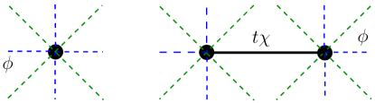
Figure 1: Single site (left) and two-site cluster (right) for the suqare lattice. Solid line shows nearest hopping within the cluster. Dashed lines represent coupling to the bath described by the order parameter $\Phi$.

Single-site mean field theory: Applying the mean field theory to a single-site “cluster”, $H_{\theta}$ for a square lattice model is reduced to a single site rotor Hamiltonian,

$$H^{\Box,(1)}_{\theta}=-8(t\chi\!\!+\!\!t^{\prime}\chi^{\prime})\Phi({\rm e}^{-i\theta}\!\!+\!\!{\rm e}^{+i\theta})\!\!+\!\!\frac{U}{2}\!(n^{\theta})^{2}\!\!-\!\!\mu_{\theta}n^{\theta}.$$ (22)

For given $\chi,\chi^{\prime}$ (obtained from the spinon problem) and charge density $\langle n^{\theta}\rangle=\delta$, we start from some trial value of $\Phi$ and diagonalize $H^{(1)}_{\theta}$ in the rotor number (angular momentum) basis $\{|n^{\theta}\rangle\}$ by truncating the rotor Hilbert space to $|n^{\theta}|\leq L$. $L$ is increased until the results converge. We found $L=2$ is accurate enough for all of our calculations. Using the ground state wavefunction $|G\rangle_{(1)}$, the ground state average $\langle n^{\theta}\rangle_{(1)}$ and $\Phi=\langle{\rm e}^{i\theta}\rangle_{(1)}$ are computed. $\mu_{\theta}$ is adjusted to give the correct charge density, and the procedure is iterated until $\Phi$ is converged. Alternatively, one may minimize the ground state energy under the charge density constraint $\langle n^{\theta}\rangle_{(1)}$ to find $\Phi$, and the result will be the same. Once $\Phi$ is determined self-consistently, we record energy eigenvalues $E_{\alpha}$ and eigen states $|\alpha\rangle$. Within the single site approximation, the rotor kinetic energy $B=B^{\prime}=\Phi^{2}$. These values will be fed into the spinon Hamiltonian as parameters. For the triangular lattice model with $t^{\prime}=0$, the corresponding single-site Hamiltonian is

$$H^{\triangle,(1)}_{\theta}=-12t\chi\Phi({\rm e}^{-i\theta}+{\rm e}^{+i\theta})+\frac{U}{2}(n^{\theta})^{2}-\mu_{\theta}n^{\theta}.$$ (23)

Two-site cluster: Going to larger cluster size yields much better approximations for the rotor kinetic energy and intersite correlations. For example, in a two site cluster model of the the square lattice problem, the Hamiltonian $H_{\theta}$ is approximated by

$$H^{\Box,(2)}_{\theta} = -2t\chi({\rm e}^{-i\theta_{1}}{\rm e}^{+i\theta_{2}}+{\rm h.c.})$$ (24)

$$- (6t\chi+8t^{\prime}\chi_{2})\Phi({\rm e}^{-i\theta_{1}}+{\rm e}^{-i\theta_{2}}+{\rm h.c.})$$

$$+ \frac{U}{2}(n^{\theta}_{1})^{2}+\frac{U}{2}(n^{\theta}_{2})^{2}-\mu_{\theta}(n^{\theta}_{1}+n^{\theta}_{2}).$$

Similar to the single site case, this Hamiltonian is diagonalized numerically in basis $\{|n^{\theta}_{1},n^{\theta}_{2}\rangle\}$ and $\Phi$ is determined self-consistently via $\Phi=|\langle{\rm e}^{\pm i\theta_{1}}\rangle_{(2)}|=|\langle{\rm e}^{\pm i\theta_{2}}\rangle_{(2)}|$, where the average is with respect to the ground state $|G\rangle_{(2)}$. Intersite correlations are obtained from the ground state wavefunction using $B\equiv\langle{\rm e}^{-i\theta_{1}}{\rm e}^{+i\theta_{2}}\rangle_{(2)}$ for nearest neighbors and $B^{\prime}\equiv\Phi^{2}$ for next nearest neighbors. These will be used in the spinon Hamiltonian. For the triangular lattice, the two site cluster Hamiltonian is given by

$$H^{\triangle,(2)}_{\theta} = -2t\chi({\rm e}^{-i\theta_{1}}{\rm e}^{+i\theta_{2}}+{\rm h.c.})$$ (25)

$$- 10t\chi\Phi({\rm e}^{-i\theta_{1}}+{\rm e}^{-i\theta_{2}}+{\rm h.c.})$$

$$+ \frac{U}{2}(n^{\theta}_{1})^{2}+\frac{U}{2}(n^{\theta}_{2})^{2}-\mu_{\theta}(n^{\theta}_{1}+n^{\theta}_{2}).$$

Finally, we note that the rotor hopping $t\chi_{ij}$ is complex in the U(1) staggered flux state. The rotor Hamiltonian in this case can be solved similarly on a two-site lattice to obtain the complex $B_{ij}$. It is straightforward to generalize this to larger clusters depending on the available computational resources.

The main qualitative difference in the results obtained from the single-site mean field theory and the cluster mean field theories is the following. In single site mean field theory, the kinetic energy $B$ is the same as the square of the order parameter, $\Phi^{2}$. Thus, it vanishes in the Mott insulating phase. This amounts to neglecting all number fluctuations within the Mott phase, and it is too crude an approximation especially when close to the Mott transition. By contrast, the cluster mean field theory does much better job capturing the short distance correlations, the kinetic energy $\propto B$ does not simply follow $\Phi^{2}$. For instance at the commensurate filling $\langle n^{\theta}_{i}\rangle=1$ and large $U/t$, deep in the Mott insulator, we find $B\sim t/U$.

VI Mott transition on the triangular lattice at half-filling

A Mott transition refers to an interaction induced transition from a conducting phase to an insulating phase. The insulating phases may or may not be accompanied by any conventional broken symmetries. One interesting recent example of such a Mott transition is the pressure induced insulator to metal transition in organic compounds such as $\kappa$-(ET)₂Cu₂(CN)₃ at an effective density of one electron per site (half-filling) shimizu ; Kurosaki . The simplest model Hamiltonian describing this material is the Hubbard model on an isotropic triangular lattice. Here we use the cluster slave rotor mean field theory to study the $T=0$ phase diagram of model Eq. (1) on a triangular lattice with $t^{\prime}=0$.

Previous exact diagonalization studies of the triangular lattice Hubbard model suggested capone a direct first order transition from a uniform metallic phase into an antiferromagnetic insulator with $120^{\circ}$ Neel order at $U/t\approx 12$. However that study also pointed out capone that a more complex phase diagram emerges from Hartree-Fock calculations which show a metallic SDW and incommensurate spiral ordering in addition to the non-magnetic metal and the antiferromagnetic insulator. However, the validity of such a weak-coupling approach is unclear for such large values of $U/t$. More recent numerical studies morita using the so-called “path integral renormalization group” (PIRG) method indicate that the ground state first undergoes a metal to spin-liquid insulator transition at a critical $U_{c}\sim 5t$. At larger $U>U_{c}$, the spin liquid phase undergoes a second transition into the $120^{\circ}$ Neel ordered antiferromagnetic state. Variational wave function studies, which attack the problem from the insulating phase, find that the $120^{\circ}$ Neel ordered insulator is unstable to a spin liquid state which may resemble a projected Fermi sea of spinons Motrunich . This spin liquid state with a Fermi sea of spinons has been argued Motrunich ; Lee-lee to provide a description of the non-magnetic insulating phase seen in $\kappa$-(ET)₂Cu₂(CN)₃.

Using the ansatz Eq. (17) for the triangular lattice, we can obtain the mean field spinon Hamiltonian

$$H^{\mathrm{fs}}_{f} =\sum_{{{\bf{k}}},\sigma}\xi_{{\bf{k}}}f^{\dagger}_{{{\bf{k}}}\sigma}f^{\vphantom{\dagger}}_{{{\bf{k}}}\sigma}-\frac{3JM}{2}\sum_{{\bf{k}}}\left(f^{\dagger}_{{{\bf{k}}}\uparrow}f^{\vphantom{\dagger}}_{{{\bf{k}}}-{\bf{Q}}\downarrow}+\mathrm{h.c.}\right),$$ (26)

$$\xi_{{\bf{k}}} =-2(tB+\frac{3J\chi}{4})(\cos k_{a}+\cos k_{b}+\cos k_{c})-\mu_{f}.$$ (27)

where $k_{a}={{\bf{k}}}\cdot\hat{a}$, $k_{b}={{\bf{k}}}\cdot\hat{b}$, and $k_{c}=k_{a}+k_{b}$. The spinon kinetic energy has contributions from the bare spinon hopping as well as from the antiferromagnetic interactions.

The excitation energy of the SDW quasiparticles is given by

$$\lambda^{\pm}_{{\bf{k}}}=\frac{\xi_{{\bf{k}}}+\xi_{{{\bf{k}}}-{\bf{Q}}}}{2}\pm\frac{1}{2}E_{{\bf{k}}},$$ (28)

$$E_{{\bf{k}}}\equiv\sqrt{(\xi_{{\bf{k}}}-\xi_{{{\bf{k}}}-{\bf{Q}}})^{2}+(3JM)^{2}}.$$ (29)

The self-consistency conditions for $M,\chi$ and the number constraint equation $\langle n_{f}\rangle=1-\delta$ (which determines $\mu_{f}$) reduce to

$$M = \frac{1}{N}\sum_{{\bf{k}}}\frac{3JM}{2E_{{\bf{k}}}}\left[\Theta(-\lambda^{-}_{{\bf{k}}})-\Theta(-\lambda^{+}_{{\bf{k}}})\right],$$ (30)

$$\chi = \frac{1}{3N}\sum_{{\bf{k}}}\left[u^{2}_{{\bf{k}}}\Theta(-\lambda^{-}_{{\bf{k}}})+v^{2}_{{\bf{k}}}\Theta(-\lambda^{+}_{{\bf{k}}})\right]$$ (31)

$$\times (\cos k_{a}+\cos k_{b}+\cos k_{c}),$$

$$1-\delta = \frac{1}{N}\sum_{{\bf{k}}}\left[\Theta(-\lambda^{+}_{{\bf{k}}})+\Theta(-\lambda^{-}_{{\bf{k}}})\right].$$ (32)

Here $\Theta(x)$ is the step function, and the coherence factor

$$u^{2}_{{\bf{k}}}=\frac{1}{2}\left[1-\frac{\xi_{{\bf{k}}}-\xi_{{{\bf{k}}}-{\bf{Q}}}}{E_{{\bf{k}}}}\right],\;\;\;v^{2}_{{\bf{k}}}=1-u^{2}_{{\bf{k}}}.$$ (33)

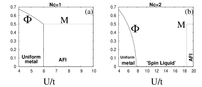
Figure 2: The rotor order parameter $\Phi$ and the sublattice magnetization $M$ as function of $U/t$ for the triangular $tUJ$ model at half filling, $J=t/4$. Left (a): Predictions of the single-site slave rotor mean field theory. The transition from the uniform metal to the antiferromagnetic insulator (AFI) is first order. Right (b): Results obtained using a 2-site rotor cluster. There is an intermediate spin liquid state in which $M$ is zero within our numerical accuracy.

The results obtained for the Mott transition with a fixed $J=t/4$ are plotted in Fig.2. We show results for the rotor order parameter $\Phi$, which distinguishes metallic ($\Phi\neq 0$) from insulating ($\Phi=0$) states, and the sublattice magnetization $M$ for the $120^{\circ}$ Neel state. Using a single-site cluster for the rotors, and computing the energy of the different states, we find the phase diagram in Fig.2(a) which shows a direct, strongly discontinuous, transition from the uniform metal into a magnetically ordered insulating state, occurring at $U/t\sim 6$. The magnetic ordering in the insulator is ‘classical’ in the sense that the ordered moment is the full moment ($M=1/2$), and the electronic kinetic energy vanishes in the insulator. By contrast, the 2-site cluster for the rotor yields a richer phase diagram as shown in Fig.2(b). It exhibits a continuous Mott transition into an insulating state at about $U/t\sim 7.8$. However the insulating state has no ordered moment, $M$ is essentially zero within our numerical accuracy. The insulating phase is thus consistent with a featureless ‘spin liquid’ described by a spinon Fermi sea. This ‘spin liquid’ state may be further unstable to spinon pairing but we have not, thus far, explored such a possibility. For larger $U/t\sim 18.5$, we find a discontinuous transition of this uniform ‘spin liquid’ state into a $120^{\circ}$ ordered antiferromagnet. This result, of a transition at large $U/t$ from the spin liquid into the ordered state, can be checked using PIRG calculations extended to larger values of $U/t$ than in Ref. morita, . Our main message is that using a cluster approach to the rotor sector leads to a significant qualitative difference with respect to a single-site mean field theory in that it leads to an insulating spin liquid phase at intermediate $U/t$.

This phase diagram is not too sensitive to the precise value of $J/t$ so long as it is not too large. For smaller values of $J/t$, the window of the ‘spin liquid’ phase extends to larger $U/t$. For much larger values of $J/t$, we find that even the larger clusters can yield a strong discontinuous transition from the metal to a magnetically ordered insulator. The details of the phase diagram in the slave rotor mean field theory are determined by the competition between the renormalized spinon kinetic energy, $\sim t^{2}/U$, and the fixed exchange constant $J$. If the Mott transition of the rotors occurs at a small $U/t$, then the renormalized spinon kinetic energy is large compared to the antiferromagnetic exchange constant $J$ and this can frustrate magnetic ordering. This is similar in spirit, although not in details, to local charge fluctuations frustrating magnetic order on the triangular lattice via ring-exchange processes. Using a variational approach to the ring-exchange model, Motrunich has shown that it can significantly suppress or completely destroy magnetic order leading to a uniform spin liquid state deficiency . A phase diagram for the triangular lattice Mott insulator with an intervening spin liquid phase is also consistent with results from numerical approaches such as the PIRG. However the metal-insulator transition point obtained in that study is at $U/t\sim 5$ indicating that our mean field result may not be quantitatively accurate.

VII d-wave superconductivity in the doped cuprate materials

High temperature superconductivity in the hole doped cuprates has been a prototypical example of how strong correlations lead to a variety of novel phenomena not observed in conventional superconductors. There are two, seemingly quite different, approaches to d-wave superconductivity in the cuprates. One approach starts from an electronic Fermi liquid and shows that antiferromagnetic spin fluctuations centered at momentum $(\pi,\pi)$ on a square lattice can mediate d-wave pairing of electrons spin-fluct ; scalapino ; miyake . The other point of view, proposed initially by Anderson, pwa-87 begins from the undoped insulating state of the cuprates and argues that this is close to forming a spin liquid with d-wave singlet pairing which naturally leads to d-wave superconductivity upon doping away from half-filling.

From the perspective of the coupled spinon-rotor theory these two approaches may be reconciled at low energy. The weak coupling spin-fluctuation calculations would, when applied to the spinon sector of the slave rotor mean field theory, predict an instability of spinons towards d-wave pairing arising from antiferromagnetic fluctuations induced by $J$. Thus, although conventional spin fluctuation theories and models such as the spin-fermion model chubukov are quite different from spin liquid based approaches, they appear to be formally identical when reinterpreted as applying to spinons rather than electrons. At low dopings, when the exchange interaction becomes much stronger than the spinon kinetic energy, the weak coupling ‘spinon pair’ may smoothly cross over into the resonating valence bond singlets of the spin liquid Mott state. Naively, this crossover is expected to happen when the kinetic energy of the doped carriers becomes comparable to the exchange energy between neighboring spins. Recent cellular DMFT calculations haule suggest that this crossover may exhibit some features of ‘local quantum criticality’.

There has been extensive work on the $tJ$ model using U(1) and SU(2) slave boson mean field (and corresponding gauge) theories baskaran ; kotliar-liu ; Lee-rmp . The slave boson mean field theory successfully captures some essential features of the high temperature superconductors, including the d-wave symmetry, the pseudogap energy scale, and the superconducting dome kotliar-liu . Despite the seemingly bold approximations involved in such a slave particle formulation, the qualitative predictions of the slave boson mean field theory agree remarkably well with more sophisticated methods like the variational wave function approach arun-prl ; arun-prb .

In this section, we apply the cluster slave rotor mean field theory to study the superconducting phase of the hole-doped square lattice $tUJ$ model. Our first purpose is to check that it can qualitatively reproduce the well known results of the $tJ$ model in the regime $U\gg t,J$. Second, we show that by solving the rotor problem, we learn about the incoherent spectrum weight associated with charge fluctuations which leads to, among other things, particle-hole tunneling asymmetry.

The d-wave pairing ansatz for the spinon sector leads to the well known Hartree-Fock-Bogoliubov Hamiltonian

$$H^{\mathrm{dsc}}_{f} = \sum_{{{\bf{k}}},\sigma}\xi_{{\bf{k}}}f^{\dagger}_{{{\bf{k}}}\sigma}f^{\vphantom{\dagger}}_{{{\bf{k}}}\sigma}-\sum_{{{\bf{k}}}}(\Delta_{{\bf{k}}}f^{\dagger}_{{{\bf{k}}}\uparrow}f^{\dagger}_{-{{\bf{k}}}\downarrow}+\mathrm{h.c.}),$$ (34)

$$\xi_{{\bf{k}}} = -2(tB+3J\chi/4)(\cos k_{x}+\cos k_{y})$$ (35)

$$- 4t^{\prime}B^{\prime}\cos k_{x}\cos k_{y}-\mu_{f},$$

$$\Delta_{{\bf{k}}} = \Delta_{0}(\cos k_{x}-\cos k_{y})/2.$$ (36)

$H_{f}^{\rm dsc}$ is diagonalized by the standard Bogoliubov transformation to yield quasiparticle excitation energies $E_{{\bf{k}}}=\sqrt{\xi^{2}_{{\bf{k}}}+\Delta^{2}_{{\bf{k}}}}$. Here $\Delta_{0}=3J|\Delta_{ij}|$ is the antinodal gap. $\Delta_{{\bf{k}}}$, $\chi$, and $\mu_{f}$ are determined self-consistently by

$$1-\delta = \frac{1}{N}\sum_{{\bf{k}}}(1-\frac{\xi_{{\bf{k}}}}{E_{{\bf{k}}}}),$$ (37)

$$1 = \frac{1}{N}\sum_{k}\frac{3J}{8E_{{\bf{k}}}}(\cos k_{x}-\cos k_{y})^{2},$$ (38)

$$\chi = \frac{1}{4N}\sum_{k}(1-\frac{\xi_{{\bf{k}}}}{E_{{\bf{k}}}})(\cos k_{x}+\cos k_{y}).$$ (39)

After self-consistency is achieved,

$$\chi^{\prime}=(2N)^{-1}\sum_{k}(1-{\xi_{{\bf{k}}}}/{E_{{\bf{k}}}})\cos k_{x}\cos k_{y}$$ (40)

is computed as input to the rotor sector.

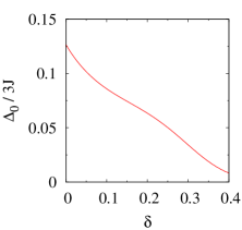
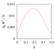
Figure 3: Doping dependence of d-wave superconductivity arising from doping a Mott insulator. Left: Maximum superconducting gap $\Delta_{0}$. Right: Superconducting order parameter $\langle c_{i\uparrow}c_{j,\downarrow}\rangle$.

We have numerically solved the coupled rotor-spinon problem for $U=12t$, $J=t/3$, $t^{\prime}=-t/4$ (these values are typical for hole doped cuprate high temperature superconductors) at doping $0\leq\delta\leq 0.4$ using a two site rotor cluster. Fig. 3 shows the doping dependence of the antinodal spinon gap $\Delta_{0}$ as well as the superconducting order parameter $\langle c_{i\uparrow}c_{j,\downarrow}\rangle=\Phi^{2}\Delta_{0}/3J$. The spinon gap decreases monotonically with increasing doping and corresponds to the psuedogap observed in high temperature superconductors. The doping dependence of the order parameter, on the other hand, takes a dome shape, reaching maximum at optimal doping $\delta\sim 0.2$. This is in accordance with the doping evolution of $T_{c}$ of high temperature superconductors. The demise of superconductivity at low doping is due to the vanishing of condensate density, which in the slave rotor formulation is proportional to $\Phi^{2}$ and goes roughly as $\delta$ at low dopings.

VII.1 Doping dependence of quasiparticle weight and nodal Fermi velocity

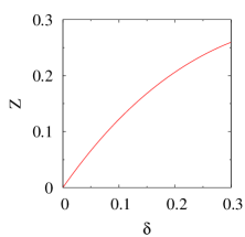
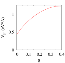
Figure 4: Quasiparticle properties of the d-wave superconductor. Left: the quasiparticle weight $Z$ obtained from slave-rotor mean field theory. Right: nodal Fermi velocity $V_{F}$ as function of doping.

Interaction effects result in a transfer of spectral weight from sharply defined coherent quasiparticles to incoherent excitations. This reduces the quasiparticle weight $Z$ from unity. Within the slave rotor mean field theory, $Z$ is given by $\Phi^{2}$ and plotted in the left panel of Fig. 4. Our slave rotor result is close to the slave boson result, as expected since $U/t\gg 1$ and the number (charge) fluctuation is suppressed. In the right panel of Fig. 4 we plot the nodal quasiparticle Fermi velocity, $v_{F}=\partial\xi_{k}/\partial k$ for $k=k_{F}$ along the nodal direction. Here in order to measure $v_{F}$ in unit of eV-$\mathrm{\AA}$ we have used $t=350$meV and a lattice spacing 3.8$\mathrm{\AA}$. We find that $v_{F}$ is a smooth function of $\delta$ and does not vanish as $\delta\to 0$. The doping dependence of $Z$ and $v_{F}$ is in qualitative agreement with experiments.

However, slave boson and slave rotor theories underestimate $Z,v_{F}$ when compared with Gutzwiller projected variational wavefunction calculations arun-prl ; arun-prb , indicating that gauge fluctuations that bind slave particles have to be taken into account to describe those calculations. Furthermore, the calculated value of $v_{F}$ is smaller (by a factor of two) compared with experiments kaminski ; lanzara , while the doping dependence of $v_{F}$ in the range $\delta\sim 0.1-0.2$ disagrees with the experimental observation lanzara that $v_{F}\simeq 1.5$eV-$\mathrm{\AA}$ is essentially completely doping independent in this range. On the other hand good agreement with experiments is achieved by variational wave function calculations arun-prl ; arun-prb . These disagreements show a shared weakness of the slave-particle mean field theories. Namely some degree of spinon-chargon interaction beyond mean field theory, arising from gauge fluctuations, needs to be retained in order to make a quantitative comparison with the photoemission experiments.

VII.2 Particle-hole asymmetry in tunneling

Tunneling experiments in the underdoped cuprate superconductors find a marked asymmetry between the tunneling conductance at positive bias (tunneling in an electron from tip to sample) versus negative bias (extracting an electron from the sample). This had been observed in earlier experiments in slightly underdoped materials Renner ; pan which focussed on the tunneling conductance at low energy. More recent experiments, which have gone to lower doping and to larger bias, have shown that this asymmetry grows significantly in the strongly underdoped regime davis-Rmap .

This asymmetry was explained by calculations using slave boson mean field theory, which pointed out that it arises from the proximity of the underdoped cuprates to a correlated insulating state at zero doping rantner . Rantner and Wen rantner ; wen-asymmetry calculated the expected tunneling spectrum assuming that the slave bosons behave as free particles with a bandwidth $\sim t$. Here we use the self-consistent slave rotor mean field theory to calculate the tunneling spectrum into the weakly doped superconducting state of the cuprates. We show that the tunneling spectrum has a coherent BCS-like form at low energies while it has significant incoherent weight at negative bias in agreement with earlier results. We also compute the ratio of the integrated (upto a cutoff) tunneling density of states at positive to that at negative bias and compare the doping and cutoff dependence of this ratio with recent tunneling experiments davis-Rmap .

Within the slave rotor mean field approach, using Eq. (4) and (5), the electron Green function factorizes into spinon and rotor Green functions. This leads to a simple qualitative picture for the electronic tunneling process — namely, tunneling an electron involves tunneling a spinon and a charge. This factorization preserves the sum rule on the electron spectral function $A({{\bf{k}}},\omega)$ that $\int_{-\infty}^{+\infty}d\omega A({{\bf{k}}},\omega)=1$. The resulting local electron Green function

$$G_{\rm e}({{\bf{r}}},i\omega_{n})=-\int_{0}^{\beta}d\tau{\rm e}^{i\omega_{n}\tau}\langle c^{\vphantom{\dagger}}_{{{\bf{r}}}\uparrow}(\tau)c^{\dagger}_{{{\bf{r}}}\uparrow}(0)\rangle$$ (41)

$$=-\int_{0}^{\beta}d\tau{\rm e}^{i\omega_{n}\tau}\frac{1}{N}\sum_{{\bf{k}}}\langle f^{\vphantom{\dagger}}_{{{\bf{k}}}\uparrow}(\tau)f^{\dagger}_{{{\bf{k}}}\uparrow}(0)\rangle\langle{\rm e}^{i\theta_{{{\bf{r}}}}(\tau)}{\rm e}^{-i\theta_{{{\bf{r}}}}(0)}\rangle.$$

In another word, on the mean field level, in order to tunnel in an electron one needs to tunnel in both a spinon and a charge. Using the Hartree-Fock-Bogoliubov mean field solution of the spinons and cluster mean field solution of the rotors, we find $G_{e}({{\bf{r}}},i\omega_{n}\to\omega+i\delta)$ at zero temperature:

$$G_{\rm e}({{\bf{r}}},\omega) = \frac{1}{N}\sum_{{{\bf{k}}},m}\left[u_{{\bf{k}}}^{2}\frac{|\langle m|{\rm e}^{-i\theta_{{\bf{r}}}}|0\rangle|^{2}}{\omega+i\delta-E_{{\bf{k}}}-({\epsilon}_{m}-{\epsilon}_{0})}\right.$$ (42)

$$+ \left.v_{{\bf{k}}}^{2}\frac{|\langle 0|{\rm e}^{-i\theta_{{\bf{r}}}}|m\rangle|^{2}}{\omega+i\delta+E_{{\bf{k}}}+({\epsilon}_{m}-{\epsilon}_{0})}\right],$$

where $|m\rangle$ refers to the $m$-th eigenstates of the rotor cluster with eigenenergy ${\epsilon}_{m}$, with $|0\rangle$ being the ground state, ${{\bf{r}}}$ is a site belonging to the cluster, $u^{2}_{{\bf{k}}}=(1+\xi_{{\bf{k}}}/E_{{\bf{k}}})/2$ and $v^{2}_{{\bf{k}}}=1-u^{2}_{{\bf{k}}}$ are the usual BCS coherence factors. This leads to the electronic tunneling density of states (TDOS) $N({{\bf{r}}},\omega)=-{\pi}^{-1}\Im G_{{{\bf{r}}},\rm e}(\omega)$,

$$N({{\bf{r}}},\omega) = |\Phi|^{2}\frac{1}{N}\sum_{k}[u^{2}_{{\bf{k}}}\delta(\omega-E_{{\bf{k}}})+v^{2}_{{\bf{k}}}\delta(\omega+E_{{\bf{k}}})]$$ (43)

$$+ \frac{1}{N}\sum_{{{\bf{k}}},m\neq 0}\left[u_{{\bf{k}}}^{2}|\langle m|{\rm e}^{-i\theta_{{\bf{r}}}}|0\rangle|^{2}\delta(\omega\!\!-\!\!E_{{\bf{k}}}\!\!-\!\!{\epsilon}_{m0})\right.$$

$$+ \left.v_{{\bf{k}}}^{2}|\langle m|{\rm e}^{+i\theta_{{\bf{r}}}}|0\rangle|^{2}\delta(\omega\!\!+\!\!E_{{\bf{k}}}\!\!+\!\!{\epsilon}_{m0})\right].$$

where ${\epsilon}_{m0}={\epsilon}_{m}-{\epsilon}_{0}$. The first term proportional to $\Phi^{2}$, called the coherent part, simply reflects the Bogoliubov quasiparticle spectrum with energy $E_{{\bf{k}}}$. It describes processes in which the tunneling charge joins the ground state (the condensate) with no energy cost. This leads to the usual V-shaped nodal spectrum at low energy characteristic of the d-wave symmetry. The second term is the incoherent part, corresponding to processes creating an incoherent charge excitation whose local energetics is well captured by the cluster mean field theory, and it dominates at high energies.

The calculated TDOS is shown in the left panel of Fig. 5 for $U=12t$, $J=t/3$, and doping $x=0.06$. Within the cluster mean field approximation, the incoherent weight consists of discrete peaks corresponding to the excitation energy levels of the rotor cluster. We have included a small Lorentzian broadening for these discrete levels. We find that the tunneling spectrum exhibits a pronounced particle-hole asymmetry: there are more significant incoherent charge excitations at negative bias than large positive bias. Roughly speaking, upon extracting an electron from the system, the nearby electrons which are within a few lattice spacings can lower their kinetic energy, by $\sim t$, by rattling around the created empty space. On the contrary, it costs a lot of energy to add electrons to the system unless one finds an unoccupied site, and hence one has little incoherent spectral weight on the positive low bias side. Qualitatively similar ideas have been proposed by others using variational wavefunctions or exact diagonalization of the $t$-$J$ model on small clusters tunnelingrefs .

This particle-hole asymmetry can be quantified by introducing the ratio mohit-sumrule $R({{\bf{r}}})$ of the positive to the negative spectral weights at a given space point ${{\bf{r}}}$,

$$R({{\bf{r}}})=\frac{\int_{0}^{\Omega_{c}}N({{\bf{r}}},E)dE}{\int_{-\infty}^{0}N({{\bf{r}}},E)dE},$$ (44)

where the cutoff $\Omega_{c}\ll U$.

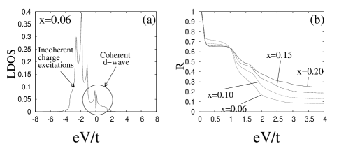
Figure 5: (a): The tunneling density of states (TDOS) at doping $x=0.06$. (b): The dependence of the particle-hole asymmetry ratio $R$ (defined in Eq. 44) on the cutoff energy $\Omega_{c}$ for a series of dopings.

The right panel of Fig. 5 shows the $\Omega_{c}$ dependence of the ratio $R$ in the doping range $x=0.06-0.2$. For small $\Omega_{c}$, it starts off close to unity for all dopings, reflecting the nearly particle-hole symmetric d-wave TDOS at low bias. Very rapidly, however, the incoherent weight present on the occupied side leads to a suppression of $R$ which plateaus at a value smaller than unity ($\sim 0.7$) with little doping dependence. This is in rough agreement with the data in Ref. davis-Rmap, . At bias $1\lesssim eV/t\lesssim 3$ there is a rapid change in $R$ versus the cutoff, beyond which all the curves appear to saturate. This is consistent with the bulk of the incoherent weight on the occupied side being centered at an energy $\sim$ 2$t$. (The wiggles in $R$ versus $\Omega_{c}$ in Fig.5 are due to the finite size cluster method.)

It has been shown out that for electronic states which obey a Gutzwiller projection constraint (two electrons are forbidden from occupying the same lattice site), there is a rigorous ‘partial sum rule’ sawatzky-sumrule which constrains the spectral weight of occupied and unoccupied states when there is a separation of scales $t\ll\Omega_{c}\ll U$. In the context of tunneling measurements, this translates mohit-sumrule into the result that the ratio of the integrated TDOS at positive bias to that at negative bias is $2\delta/(1-\delta)$ where $\delta$ is the density of doped holes mohit-sumrule ; pwa-asymmetry . Furthermore, the ratio $R({{\bf{r}}})$ has the advantage that the unknown tunneling matrix elements that determine the relation between the TDOS and the measured conductance, which can depend on the coordinate ${{\bf{r}}}$, cancel out mohit-sumrule (assuming they are energy independent). This ‘partial sum rule’ can then be used to estimate the hole density locally from tunneling experiments on doped Mott insulators mohit-sumrule ; davis-Rmap . The slave boson and rotor mean field theories violate this ‘partial sum rule’ since the spinons and rotors are assumed to be independent particles at mean field level. For $U/t\to\infty$, the ratio $R$ thus saturates, as a function of $\Omega_{c}$, to a value which is close to $\delta(1+\delta)/(1-\delta)^{2}$. This violation is expected to be fixed by including gauge fluctuations about the mean field theory lee-sumrule-fixing .

VIII Correlated normal states in a weakly doped Mott insulator on the square lattice

The finite temperature normal state of underdoped high temperature superconductors, for $T>T_{c}$, is the least understood part of the phase diagram. It exhibits pseudogap phenomenon and highly anomalous thermodynamic and transport properties. It has been suggested that understanding the underlying $T=0$ normal state in this regime might shed light on the pseudogap phenomena. Very recent experiments by Doiron-Leyraud et al Taillefer-pockets have begun to access this ground state in clean crystals of underdoped oxygen-ordered YBa₂Cu₃O_6.5. Applying high magnetic fields, in the range $\sim 40$-$60$T, to suppress superconductivity, they discovered quantum oscillations in the electrical resistance at low temperatures. This discovery can be most simply understood by postulating a well-defined Fermi surface made of small pockets in the field induced normal ground state. The authors argue that the data is less consistent with a specific band structure feature band of ortho-II YBCO, and more in line with a state with broken symmetry giving rise to Fermi surface reconstruction. This state is supposed to compete with superconductivity, to be close in energy to the superconducting state, and to show up as the ground state when superconductivity is strongly suppressed.

Several such candidate states have been proposed. One is the commensurate SDW at ordering vector $(\pi,\pi)$, which has been argued to be relevant to the electron doped cuprate superconductors millis . Given the proximity to the antiferromagnetic Neel phase at low doping, it is likely that SDW is stabilized and extends to higher doping under high fields. This is supported for example by the observation of antiferromagnetism inside the vortex cores mitrovic-nmr ; core-nmr and from theoretical studies of the vortex structure using Bogoliubov-deGennes (BdG) equations ghosal . Another candidate is the U(1) staggered flux state marston-flux (also known as the DDW state ddw-nayak ; ddw ). This state is also well known to be close in energy with the d-wave superconducting state ivanov-lee and has been advocated by Patrick Lee and collaborators to describe the pseudogap phase Lee-rmp .

In this section we study the SDW state and the U(1) staggered flux state using cluster slave rotor mean field theory. We then compute the expected cyclotron mass $m^{*}$ for each state as a function of doping, and compare them with the experiment of Doiron-Leyraud et al Taillefer-pockets . We show that by studying the doping dependence of the $m^{*}$ one can, in principle, unambiguously differentiate between these two scenarios for the normal state. We also suggest a possible resolution for the observed difference Taillefer-pockets between the hole density as inferred from the quantum oscillation measurements and from the $T_{c}$ value.

VIII.1 Spin density wave state

Applying the SDW ansatz Eq. (19), we obtain the mean field spinon Hamiltonian

$$H_{\rm afm} = \sum_{{{\bf{k}}}\sigma}\xi_{{\bf{k}}}f^{\dagger}_{{{\bf{k}}}\sigma}f^{\vphantom{\dagger}}_{{{\bf{k}}}\sigma}-2Jm\sum_{{{\bf{k}}}}\left(f^{\dagger}_{{{\bf{k}}}\uparrow}f^{\vphantom{\dagger}}_{{{\bf{k}}}+{\bf{Q}}\uparrow}\right.$$ (45)

$$- \left.f^{\dagger}_{{{\bf{k}}}\downarrow}f^{\vphantom{\dagger}}_{{{\bf{k}}}+{\bf{Q}}\downarrow}\right),$$

where we have defined

$$\xi_{{\bf{k}}} = -2(tB+3J\chi/4)(\cos k_{x}+\cos k_{y})$$ (46)

$$- 4t^{\prime}B^{\prime}\cos k_{x}\cos k_{y}-\mu_{f},$$

$$\lambda_{{\bf{k}}}^{\pm} = \frac{1}{2}\left(\xi_{{\bf{k}}}+\xi_{{{\bf{k}}}+{\bf{Q}}}\right)\pm\frac{1}{2}E_{{\bf{k}}},$$ (47)

$$E_{{\bf{k}}} = \sqrt{(\xi_{{\bf{k}}}-\xi_{{{\bf{k}}}+{\bf{Q}}})^{2}+(4Jm)^{2}}.$$ (48)

The mean field self-consistency conditions then read

$$1 = \frac{1}{N}\sum_{{{\bf{k}}}}\frac{2J}{E_{{\bf{k}}}}\left[\Theta(-\lambda_{{\bf{k}}}^{-})-\Theta(-\lambda_{{\bf{k}}}^{+})\right],$$ (49)

$$1-\delta = \frac{1}{N}\sum\left[\Theta(-\lambda_{{\bf{k}}}^{-})+\Theta(-\lambda_{{\bf{k}}}^{+})\right],$$ (50)

$$\chi = \frac{1}{4N}\sum_{{\bf{k}}}\left(\frac{\xi_{{\bf{k}}}-\xi_{{{\bf{k}}}+{\bf{Q}}}}{E_{{\bf{k}}}}\right)\left(\cos k_{x}+\cos k_{y}\right)$$ (51)

$$\times \left[\Theta(-\lambda_{{\bf{k}}}^{-})-\Theta(-\lambda_{{\bf{k}}}^{+})\right].$$

After self-consistency is achieved, we can calculate the second neighbor spinon hopping amplitude using

$$\chi^{\prime}=\frac{1}{2N}\sum_{{\bf{k}}}\cos k_{x}\cos k_{y}\left[\Theta(-\lambda_{{\bf{k}}}^{-})+\Theta(-\lambda_{{\bf{k}}}^{+})\right].$$ (52)

and use this in solving the rotor model.

In Fig.6 we plot the sublattice magnetization $M$ as function of doping predicted by the cluster slave rotor mean field theory. $M$ starts at the classical Neel state value $1/2$ at half filling and drops monotonically with increasing doping and vanishes at $\delta\sim 0.17$. The doped SDW state has four Fermi pockets centered at the nodal points ${{\bf{k}}}_{n}=(\pm\pi/2,\pm\pi/2)$. Naively, from a weak-coupling picture, one expects additional electron-like pockets centered around the $(\pi,0)$ point for small doping. We find that these do not appear in our self-consistent ground state, suggesting that the weak coupling argument does not work in this regime. Consistent with this, the area enclosed by the hole pockets around $(\pi/2,\pi/2)$ satisfies the Luttinger’s theorem for a broken symmetry state with a doubled unit cell.

VIII.2 Staggered Flux state

The U(1) staggered flux ansatz Eq. (20) leads to the mean field spinon Hamiltonian

$$H_{\rm flux}=-\sum_{{{\bf{k}}},\sigma}\left[\frac{D_{{\bf{k}}}}{2}(f^{\dagger}_{{{\bf{k}}},\sigma}+f^{\dagger}_{{{\bf{k}}}+{\bf{Q}},\sigma})(f_{{{\bf{k}}},\sigma}-f_{{{\bf{k}}}+{\bf{Q}},\sigma})+\mathrm{h.c.}\right]$$

$$-(t^{\prime}B^{\prime}\gamma^{\prime}_{{\bf{k}}}+\mu_{f})\sum_{{{\bf{k}}},\sigma}(f^{\dagger}_{{{\bf{k}}},\sigma}f_{{{\bf{k}}},\sigma}+f^{\dagger}_{{{\bf{k}}}+{\bf{Q}},\sigma}f_{{{\bf{k}}}+{\bf{Q}},\sigma}),$$ (53)

where $\gamma^{\prime}_{{\bf{k}}}=4\cos k_{x}\cos k_{y}$, and the complex hopping

$$D_{{\bf{k}}}\equiv\sum_{\hat{\delta}=\pm\hat{x},\pm\hat{y}}(tB_{i,i+\hat{\delta}}+\frac{3J}{4}\chi_{i+\hat{\delta},i}).$$ (54)

$H_{\rm flux}$ is easily diagonalized to yield the the energy spectrum, $E^{\pm}_{{\bf{k}}}=-t^{\prime}B^{\prime}\gamma^{\prime}_{{\bf{k}}}-\mu_{f}\pm|D_{{\bf{k}}}|$. The “$+$” and the “$-$” branch touches each other at the nodal points ${{\bf{k}}}_{n}$ regardless the values of staggered flux, and the low energy excitations are massless Dirac fermions. In the doping regime of our interest only the “$-$” branch is occupied. The spinon chemical potential $\mu_{f}$ and the complex “order parameter” $\chi\equiv\chi_{i,i\pm\hat{x}}=\chi^{*}_{i,i\pm\hat{y}}$ are found by solving the following self-consistency equations

$$1-\delta=\frac{1}{N}\sum_{{{\bf{k}}}}[\Theta(-E^{+}_{{\bf{k}}})+\Theta(-E^{-}_{{\bf{k}}})],$$ (55)

$$\chi=\frac{1}{2N}\sum_{{\bf{k}}}\cos k_{x}\frac{D^{*}_{{\bf{k}}}}{|D_{{\bf{k}}}|}[\Theta(-E^{-}_{{\bf{k}}})+\Theta(-E^{+}_{{\bf{k}}})].$$ (56)

Here the sum over ${{\bf{k}}}$ is within the reduced Brillouin zone, and $N$ is the number of sites on each sublattice. Finally, $\chi^{\prime}$ is obtained by

$$\chi^{\prime}=\frac{1}{2N}\sum_{{\bf{k}}}\cos k_{x}\cos k_{y}[\Theta(-E^{+}_{{\bf{k}}})+\Theta(-E^{-}_{{\bf{k}}})].$$ (57)

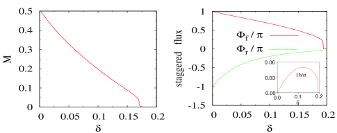
Figure 6: Left: The sublattice magnetization $M$ in the SDW normal state. Right: The spinon and rotor fluxes in the U(1) staggered flux (or DDW) state. Inset shows the electron current on a nearest neighbor bond in units of $et/\hbar$ versus doping.

With self-consistency achieved in the coupled rotor-spinon problem, we obtain $\chi=|\chi|e^{\Phi_{f}/4}$ and $B=|B|e^{\Phi_{r}/4}$, where $\Phi_{f}$ is the spinon flux per plaquette and $\Phi_{r}$ is the rotor flux (we work in a symmetric gauge, e.g., $B_{i,i\pm\hat{x}}=B^{*}_{i,i\pm\hat{y}}$). The orbital bond current

$$I=\frac{iet}{\hbar}\sum_{\sigma}\langle c^{\dagger}_{i+x,\sigma}c_{i,\sigma}-h.c.\rangle=\frac{4et}{\hbar}|\chi B|\sin(\frac{\Phi_{f}}{4}+\frac{\Phi_{r}}{4})$$ (58)

can be taken as the order parameter of the U(1) staggered flux (or DDW) phase. Fig.6 shows the doping dependence of $\Phi_{f}$, $\Phi_{r}$, and the magnitude of the orbital current. At half filling the system is in the $\pi$ flux state, $\Phi_{f}$ and $\Phi_{r}$ have the same magnitude $\pi$ but opposite sign, accordingly the bond current is zero. The current $I$ increases with doping, reaching maximum at $\delta\simeq 0.12$. For a single plaquette, the maximal bond current corresponds approximately to a magnetic field of $150$ Gauss at the center of the plaquette. $I$ drops to zero around $\delta\sim 0.2$, where the U(1) staggered flux state gives way to the Fermi liquid state and both $\Phi_{r}$ and $\Phi_{f}$ vanish. The total area enclosed by the hole pockets increase linearly with doping at small doping and is consistent with Luttinger’s theorem for a broken symmetry state with a doubled unit cell.

VIII.3 Cyclotron mass

We next discuss whether the quantum oscillation measurements of Ref. Taillefer-pockets, can shed more light on the non-superconducting normal state at low doping, and, in particular, distinguish between a commensurate SDW metal and the U(1) staggered flux (or DDW) state. The quantum oscillation data offer two pieces of information if the field induced normal state is a conventional Fermi liquid. (although more exotic possibilities cannot be ruled out rkaul ; altman ). The first is the area of the hole pocket which is obtained from the oscillation frequency, and the second is the cyclotron mass which is obtained from the temperature dependence of the oscillation amplitude and which is related to the density of states at the Fermi level. In our calculations, both the SDW and the U(1) staggered flux state have hole pocket areas consistent with the Luttinger theorem for a broken symmetry state with a doubled unit cell and this information cannot be used to discriminate between them. We therefore turn to a calculation of the cyclotron mass in these two states to compare with experiments.

The cyclotron effective mass $m^{*}$ is related to the density of states at the Fermi level in a Fermi liquid state,

$$m^{*}=N_{0}\frac{2\pi\hbar^{2}}{ta^{2}}.$$ (59)

Here $N_{0}$ is the density of states per hole pocket per spin at the Fermi level measured in units of $1/ta^{2}$. As before, we set the hopping $t=350$meV and the Cu-Cu lattice spacing $a=3.8\mathrm{\AA}$. The doping dependence of $m^{*}$ in the SDW state is shown in the left panel of Fig.7. The SDW state is characterized by a diverging $m^{*}$ as $\delta\rightarrow 0$. This reflects the classical character of the magnetically ordered insulator at $\delta=0$, namely the staggered magnetization of the insulator in the mean field theory is $M=0.5$ and the spinon kinetic energy is zero. This leads to a divergent effective mass for $\delta\to 0$. Spin fluctuations beyond mean field theory are expected to cut off this divergence; nevertheless the mass is expected to be a strongly increasing function as $\delta$ decreases. The peak in $m^{*}$ around $\delta\sim 0.17$ is a feature associated with the vanishing of the SDW order and arises from the large density of states around the $(\pi,0)$ point. The magnitude of $m^{*}$ in the range $\delta=0.1$-$0.15$ is around $4.5m_{0}$ ($m_{0}$ being the bare electron mass), in apparent disagreement with the experimental value $~{}1.9m_{0}$.

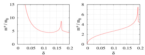
Figure 7: Cyclotron mass in units of the bare electron mass in the SDW state (left) and the U(1) staggered flux (or DDW) state (right).

The doping evolution of the cyclotron effective mass $m^{*}$ in the U(1) staggered flux (DDW) state is shown in the right panel of Fig.7. This state is characterized by a square root increase of $m^{*}$, i.e. $m^{*}\propto\sqrt{\delta}$, at small doping. This is a direct consequence of the linear Dirac spectrum at low energies and therefore a linear density of states. Again, the peak feature at $\delta\sim 0.18$ is associated with the sudden disappearance of the staggered flux state. The value of $m^{*}\simeq 3m_{0}$ at $\delta=0.1$ is closer to the experiment result $~{}1.9m_{0}$.

While a comparison of the cyclotron effective mass with experiments may seem to favor the staggered flux state over the SDW state as a normal state candidate, we cannot rule out the SDW scenario based on this quantitative comparison. As we have seen in previous sections, slave particle theory is not quantitatively accurate at the mean field level and underestimates the nodal $v_{F}$ in the superconducting state by a factor of two at $\delta=0.1$. To distinguish these two scenarios, it is more useful to study the doping dependence of $m^{*}$. From Fig.7 we observe that the effective cyclotron mass in the SDW state and the staggered flux state have almost opposite doping dependences, we propose that measurements of $m^{*}$ at a series of nearby dopings, especially at smaller $\delta$, may help to identify which candidate normal state is realized.

Finally, the experiments Taillefer-pockets find a difference between the carrier densities as inferred from the quantum oscillation period and from $T_{c}$. Assuming 2 hole pockets in a reduced Brillouin zone, which is consistent with a SDW or a U(1) staggered flux state, the oscillation period leads to an estimate $\delta\sim 0.075$ while the value estimated from $T_{c}$ is closer to $\delta\sim 0.1$. This discrepancy Taillefer-pockets , an apparently significant violation of the Luttinger count, can be accounted for in several ways including a possible bilayer splitting nicolas . However, the bilayer splitting is expected to be very small at low doping due to renormalization by strong correlation effects. We offer another plausible explanation for this discrepancy. The field induced ‘normal state’ is likely to contain vortices, which can be inferred from the sign change, with temperature, of the Hall coefficient, a feature which is seen in the mixed state in other cuprate materials and at other dopings hagen . It has been suggested that the underlying normal state of the cuprates should appear in the vicinity of such vortices vortexcore . However, it has also been found in BdG calculations ghosal of the structure of a single vortex that the density around the vortex is not uniform. At low doping and even in the presence of moderate Coulomb interactions ghosal , the density appears to be depleted within the vortex core and piled up as a screening cloud at some distance away from the core, with the far region being superconducting and at the bulk density. If the normal state being explored arises from the depleted core region, the observed density could deviate from the bulk density in the correct direction. Testing this explanation calls for further experiments as well as detailed theoretical calculations of the vortex structure.

VIII.4 Implications for Fermi arcs

We end this section by commenting on the relation between the hole pockets revealed in the low temperature quantum oscillation experiments and the Fermi arcs observed in the high temperature normal state above $T_{c}$ in photoemission experiments. Assuming that the field induced normal state has hole pockets, it has been suggested that the Fermi arcs seen in photoemission studies arcsexpts may be just these hole pockets. However, the quantum oscillation experiments are carried out at rather high magnetic fields $B\sim 50T$ at very low temperature $T\ll T_{c}$, while the photoemission experiments are done in zero magnetic field and at fairly high temperatures $T\sim 40-200K$. Given this, there is no a priori reason to expect that the photoemission experiments are accessing the properties of such an underlying normal ground state. The Fermi arcs seen in the photoemission experiments seem to be more consistent with fluctuating d-wave superconductivity arcs1 ; arcs2 . In particular, earlier work by us arcs1 suggests an explanation which relies on phenomenological spin charge separation ideas, quite close to the route explored in this paper, and provides a possible explanation for Fermi arcs whose length scales $~{}T/T^{*}$, where $T^{*}$ is the pseudogap temperature. Current photoemission experiments do not appear to have the resolution to settle the issue of whether the arcs indeed arise from hole pockets. We suggest that further high resolution photoemission experiments could focus on the momentum distribution of the low energy spectral weight (integrated from zero to some small energy). It would be useful to check whether this spectral weight tends to be centered at momenta corresponding to the low temperature d-wave nodes of the SC, or whether it tends to shift away towards some underlying hole pocket Fermi surface once the system is heated to temperatures above $T_{c}$.

IX Discussion

We have formulated a cluster slave rotor mean field theory of strongly interacting electronic systems, which extends earlier work of Florens and Georges Florens . In this formulation, the rotor sector and spinon sector are coupled to each other by self-consistency equations, and the rotor Hamiltonian is solved on a finite cluster self-consistently coupled to an order parameter bath (rest of the lattice). The main advantage of the cluster mean field theory lies in that the short range correlation functions of the rotors is properly taken into account. By applying it to several examples, we have shown that this method provides a unified framework to study strongly correlated electronic systems. Although we only focused on zero temperature, it is straight forward to generalize the theory to finite temperature. Extensions to inhomogeneous states are also likely to be of interest.

One shortcoming of the cluster mean field theory for the rotor sector is that, by working with finite clusters coupled to a static bath, we freeze the Goldstone modes (phase fluctuations). Such Goldstone mode fluctuations can be explicitly retained in complementary methods such as the random phase approximation sheshadri or other approaches huber to the rotor sector. These methods of solving the rotor problem can be combined with the spinon sector to formulate the self-consistent slave rotor mean field theory erhaiunpub .

In the path integral formulation of the slave rotor approach Florens ; Lee-lee ; kim , our mean field theory is equivalent to a saddle point approximation which ignores the gauge field fluctuations. Such fluctuations beyond mean field theory are expected to introduce effective interactions between slave particles to yield the correct low energy sum rules lee-sumrule-fixing including the ‘partial sum rule’ for the particle-hole asymmetry ratio $R$. These will be explored elsewhere erhaiunpub .

Note added: After our paper was submitted, some related works have appeared on the arxiv. The self-consistent cluster mean field theory for bosons has been shown to successfully describe the supersolid phase and the phase diagram of bosons on a triangular lattice hassan . Two further experiments carried out on YBa₂Cu₄O₈ (hole doping $\sim 0.15$) have also found evidence of Shubnikov-de Haas oscillations Yelland ; Bangura in a magnetic field with a larger cyclotron mass, $m^{*}\sim 2.7-3m_{e}$, than in ortho-II YBCO. A recent preprint by Chen et al discusses the field induced antiferromagnetic metallic ground state in the underdoped cuprates zhang-rice . Their principal result is the relation between the quantum oscillation frequency and the hole doping in this state and it is in agreement with our conclusion. Various proposals for interpreting the Fermi arcs above $T_{c}$, as well as their connection to the hole pockets in ground state, have been examined recently by Harrison et al harrison and Norman et al norman-arc .

- (1) E. Dagotto, Rev. Mod. Phys. 66, 763 - 840 (1994).
- (2) A. Georges, G. Kotliar, W. Krauth, and M. J. Rozenberg, Rev. Mod. Phys. 68, 13 (1996).
- (3) T. Maier, M. Jarrell, T. Pruschke, and M. H. Hettler, Rev. Mod. Phys. 77, 1027 (2005).
- (4) B. Kyung, S. S. Kancharla, D. Senechal, A.-M. S. Tremblay, M. Civelli, G. Kotliar, Phys. Rev. B73, 165114 (2006).
- (5) S. S. Kancharla, M. Civelli, M. Capone, B. Kyung, D. Senechal, G. Kotliar, A.-M.S. Tremblay, cond-mat/0508205.
- (6) F. C. Zhang, C. Gros, T. M. Rice, and H. Shiba, Supercond. Sci. Technol. 1, 36 (1988).
- (7) P. W. Anderson, P. A. Lee, M. Randeria, T. M. Rice, N. Trivedi, and F. C. Zhang, J. Phys. Condens. Matter 16, R755 (2004).
- (8) G. Baskaran, Z. Zou, and P. W. Anderson, Solid State Comm. 63, 973 (1987).
- (9) P. Coleman, Phys. Rev. B 29, 3035 (1984).
- (10) G. Kotliar and J. Liu, Phys. Rev. B 38, 5142 (1988).
- (11) P. A. Lee, N. Nagaosa and X.-G. Wen, Rev. Mod. Phys. 78 (2006).
- (12) S. Florens and A. Georges, Phys. Rev. B 70, 035114 (2004).
- (13) N. Read and S. Sachdev, Phys. Rev. Lett. 66, 1773 (1991); X. G. Wen, Phys. Rev. B44, 2664 (1991); T. Senthil and M. P. A. Fisher, Phys. Rev. B62, 7850 (2000).
- (14) M. P. A. Fisher, P. B. Weichman, G. Grinstein, D.S. Fisher, Phys. Rev. B 40, 546 (1989).
- (15) K. Sheshadri, H. R. Krishnamurthy, R. Pandit, and T. V.Ramakrishnan, Europhys. Lett. 22, 257 (1993).
- (16) Y. Shimizu, K. Miyagawa, K. Kanoda, M. Maesato, and G. Saito, Phys. Rev. Lett. 91, 107001 (2003).
- (17) Y. Kurosaki, Y. Shimizu, K. Miyagawa, K. Kanoda, and G. Saito, Phys. Rev. Lett. 95, 177001 (2005).
- (18) Y. Kohsaka, C. Taylor, K. Fujita, A. Schmidt, C. Lupien, T. Hanaguri, M. Azuma, M. Takano, H. Eisaki, H. Takagi, S. Uchida, and J. C. Davis, Science 315, 1380 (2007).
- (19) J. B. Marston and I. Affleck, Phys. Rev. B 39, 11538 (1989).
- (20) F. C. Zhang, Phys. Rev. Lett. 90, 207002 (2003).
- (21) B. J. Powell and R. H. McKenzie, Phys. Rev. Lett. 94, 047004 (2005).
- (22) S.-S. Lee and P. A. Lee, Phys. Rev. Lett. 95, 036403 (2005).
- (23) P. Monthoux and D. Pines, Phys. Rev. Lett. 69, 961 (1992).
- (24) D. J. Scalapino, E. Loh, and J. E. Hirsch, Phys. Rev. B 34, 8190 (1986).
- (25) K. Miyake, S. Schmitt-Rink, and C. M. Varma, Phys. Rev. B 34, 6554 (1986).
- (26) M. Capone, L. Capriotti, F. Becca, and S. Caprara, Phys. Rev. B 63, 085104 (2001).
- (27) H. Morita, S. Watanabe, and M. Imada, J. Phys. Soc. Jpn. 71, 2109 (2002).
- (28) O. Parcollet, G. Biroli, and G. Kotliar, Phys. Rev. Lett. 92, 226402 (2004).
- (29) J. Liu, J. Schmalian, and N. Trivedi, Phys. Rev. Lett. 94, 127003 (2005).
- (30) J. Y. Gan, Y. Chen, Z. B. Su, and F. C. Zhang, Phys. Rev. Lett. 94, 067005 (2005).
- (31) B. Kyung and A.-M. S. Tremblay, Phys. Rev. Lett. 97, 046402 (2006).
- (32) K. Aryanpour, W. E. Pickett, and R. T. Scalettar, Phys. Rev. B 74, 085117 (2006).
- (33) O. I. Motrunich, Phys. Rev. B 72, 045105 (2005); ibid 73, 155115 (2006).
- (34) D. A. Ivanov, P. A. Lee, Phys. Rev. B 68, 132501 (2003).
- (35) C. Nayak, Phys. Rev. B 62, 4880 (2000).
- (36) S. Chakravarty, R. B. Laughlin, D. K. Morr, and C. Nayak, Phys. Rev. B 63, 094503 (2001).
- (37) It is a deficiency of our mean field slave rotor approach that the value of has to be seperately specified, and multispin interactions, which arise naturally within a perturbation theory in the insulating phase of the Hubbard model, would need to be included by hand. However, the advantage of the mean field theory is that we can address the Mott insulator transition while the perturbation is necessarily restricted to the insulating phase.
- (38) P. W. Anderson, Science 235, 1196 (1987).
- (39) M. Henty, A. V. Chubukov and D. Morr, Phys. Repts. 288, 355 (1997); A. V. Chubukov and M. R. Norman, Phys. Rev. B70, 174505 (2004).
- (40) K. Haule and G. Kotliar, cond-mat/0605149.
- (41) A. Paramekanti, M. Randeria, and N. Trivedi, Phys. Rev. Lett. 87, 217002 (2001).
- (42) A. Paramekanti, M. Randeria, and N. Trivedi, Phys. Rev. B 70, 054504 (2004).
- (43) A. Kaminski, J. Mesot, H. Fretwell, J. C. Campuzano, M. R. Norman, M. Randeria, H. Ding, T. Sato, T. Takahashi, T. Mochiku, K. Kadowaki, and H. Hoechst, Phys. Rev. Lett. 84, 1788 (2000); A. Kaminski, M. Randeria, J. C. Campuzano, M. R. Norman, H. Fretwell, J. Mesot, T. Sato, T. Takahashi, and K. Kadowaki, Phys. Rev. Lett. 86, 1070 (2001).
- (44) X. J. Zhou, T. Yoshida, A. Lanzara, P. V. Bogdanov, S. A. Kellar, K. M. Shen, W. L. Yang, F. Ronning, T. Sasagawa, T. Kakeshita, T. Noda, H. Eisaki, S. Uchida, C. T. Lin, F. Zhou, J. W. Xiong, W. X. Di, Z. X. Zhao, A. Fujimori, Z. Hussain, and Z. X. Shen, Nature 423, 398 (2003).
- (45) N. Doiron-Leyraud, C. Proust, D. LeBoeuf, J. Levallois, J.-B. Bonnemaison, R. Liang, D. A. Bonn, W. N. Hardy, and L. Taillefer, Nature 447, 565 (2007).
- (46) R. Kaul, Y.-B. Kim, S. Sachdev and T. Senthil, cond-mat/0706.2187
- (47) E. Altman, private communication.
- (48) We thank N. Doiron-Leyraud and L. Taillefer for a discussion of this point.
- (49) S. J. Hagen, C. J. Lobb, R. L. Greene, and M. Eddy, Phys. Rev. B43, 6246 (1991); T. R. Chien, T. W. Jing, N. P. Ong, and Z. Z. Wang, Phys. Rev. Lett. 66, 3075 (1991).
- (50) P. A. Lee and X. G. Wen, Phys. Rev. B63, 224517 (2001); M. M. Maska, M. Mierzejewski, Phys. Rev. B68, 024513 (2003); A. Ghosal, C. Kallin, and A. J. Berlinsky, Phys. Rev. B66, 214502 (2002); Q.-H. Wang, J. H. Han, and D.-H. Lee, Phys. Rev. Lett. 87, 167004 (2001).
- (51) M. R. Norman, H. Ding, M. Randeria, J. C. Campuzano, T. Yokoya, T. Takeuchi, T. Takahashi, T. Mochiku, K. Kadowaki, P. Guptasarma, D. G. Hinks, Nature 392, 157 (1998); A. Kanigel, M. R. Norman, M. Randeria, U. Chatterjee, S. Suoma, A. Kaminski, H. M. Fretwell, S. Rosenkranz, M. Shi, T. Sato, T. Takahashi, Z. Z. Li, H. Raffy, K. Kadowaki, D. Hinks, L. Ozyuzer, J. C. Campuzano, Nature Physics 2, 447 (2006).
- (52) A. Paramekanti and E. Zhao, Phys. Rev. B75, R140507 (2007).
- (53) E. Berg and E. Altman, cond-mat/0705.1566 (unpublished).
- (54) Ch. Renner, B. Revaz, J.-Y. Genoud, K. Kadowaki, and Ø. Fischer, Phys. Rev. Lett. 80, 149 (1998).
- (55) S. H. Pan, E. W. Hudson, K. M. Lang, H. Eisaki, S. Uchida, and J. C. Davis, Nature 403, 746 (2000).
- (56) W. Rantner and X.-G. Wen, Phys. Rev. Lett. 85, 3692 (2000).
- (57) T. C. Ribeiro, X.-G. Wen, Phys. Rev. Lett. 97, 057003 (2006).
- (58) M. B. J. Meinders, H. Eskes, and G. A. Sawatzky, Phys. Rev. B 48, 3916 (1993).
- (59) H.-Y. Yang, F. Yang, Y.-J. Jiang and T. Li, cond-mat/0604488; C.-P. Chou, T. K. Lee and C.-M. Ho, Phys. Rev. B74, 092503 (2006).
- (60) M. Randeria, R. Sensarma, N. Trivedi, and F.-C. Zhang, Phys. Rev. Lett. 95, 137001 (2005).
- (61) P.W. Anderson and N.P. Ong, J. of Phys. and Chem. of Solids 67, 1 (2006).
- (62) P. A. Lee, N. Nagaosa, T.-K. Ng, and X.-G. Wen, Phys. Rev. B 57, 6003 (1998).
- (63) E. Bascones, T. M. Rice, A. O. Shorikov, A. V. Lukoyanov, and V. I. Anisimov, Phys. Rev. B 71, 012505 (2005).
- (64) J. Lin and A. J. Millis, Phys. Rev. B 72, 214506 (2005).
- (65) V. F. Mitrovic, E. E. Sigmund, M. Eschrig, H. N. Bachman, W. P. Halperin, A. P. Reyes, P. Kuhns, and W. G. Moulton, Nature 413, 501 (2001).
- (66) K. Kakuyanagi, K. Kumagai, Y. Matsuda, and M. Hasegawa, Phys. Rev. Lett. 90, 197003 (2003).
- (67) D. Knapp, C. Kallin, A. Ghosal, S. Mansour, Phys. Rev. B71, 064504 (2005).
- (68) K.-S. Kim, Phys. Rev. Lett. 97, 136402 (2006).
- (69) S. D. Huber, E. Altman, H. P. Büchler, and G. Blatter, Phys. Rev. B 75, 085106 (2007).
- (70) E. Zhao, unpublished.
- (71) E. A. Yelland, J. Singleton, C. H. Mielke, N. Harrison, F. F. Balakirev, B. Dabrowski, and J. R. Cooper, arXiv:0707.0057v1 [cond-mat.supr-con], unpublished.
- (72) A. F. Bangura, J. D. Fletcher, A. Carrington, J. Levallois, M. Nardone, B. Vignolle, P. J. Heard, N. Doiron-Leyraud, D. LeBoeuf, L. Taillefer, S. Adachi, C. Proust, and N. E. Hussey, arXiv:0707.4461v1 [cond-mat.supr-con], unpublished.
- (73) S. R. Hassan, L. de Medici, and A.-M.S. Tremblay, arXiv:0707.0866v1 [cond-mat.str-el], unpublished.
- (74) W.-Q. Chen, K.-Y. Yang, T. M. Rice, and F. C. Zhang, arXiv:0706.3556v2 [cond-mat.supr-con], unpublished.
- (75) N. Harrison, R. D. McDonald, and J. Singleton, arXiv:0708.2924v1 [cond-mat.supr-con], unpublished.
- (76) M. R. Norman, A. Kanigiel, M. Randeria, U. Chatterjee, and J. C. Campuzano, arXiv:0708.1713v1, unpublished.