Sine-Gordon solitons, auxiliary fields, and singular limit of a double pendulums chain

Summary. We consider the continuum version of an elastic chain supporting topological and non-topological degrees of freedom; this generalizes a model for the dynamics of DNA recently proposed and investigated by ourselves. In a certain limit, the non-topological degrees of freedom are frozen, and the model reduces to the sine-Gordon equations and thus supports well-known topological soliton solutions. We consider a (singular) perturbative expansion around this limit and study in particular how the non-topological field assume the role of an auxiliary field. This provides a more general framework for the slaving of this degree of freedom on the topological one, already observed elsewhere in the context of the mentioned DNA model; in this framework one expects such phenomenon to arise in a quite large class of field-theoretical models.

1 Introduction

In a recent paper [1] we analyzed a “composite” model of DNA torsion dynamics, pretty much in the spirit of the by now classical Peyrard-Bishop, Yakushevich and Barbi-Cocco-Peyrard models [2, 3, 4, 5, 6, 7, 8, 9, 10]; this model amounted to a field-theoretic Lagrangian with topological and non-topological interacting fields. We studied in particular the solitary wave excitations (we call these solitons for ease of language) it supports; this analysis displayed some puzzling and somehow surprising features:

• on the one hand, the speed of given soliton solutions of a certain (relevant) type is not a free parameter but turns out to be fixed by (the parameters of) the model;

• On the other hand, when performing a perturbative analysis (exact solution of the model was not possible) the non-topological field turns out to be completely determined – we say then it is slaved – by the topological one.

It appeared that these phenomena are – rather obviously – not specific to the model considered there, nor to DNA dynamics, but actually common to a much wider class of models; they could also be of rather obvious interest in applications. We believe therefore they are worth further investigation and clarification.

In a previous related paper [11] we have investigated the selection of the soliton speed, i.e. point (a) above; in the present paper we focus on point (b), i.e. on the slaving of one field. We identify the origin of this in the remarkable fact that the slaved field, while being on equal footing in the full theory, becomes an auxiliary field in the perturbative expansion; that is, at each order in the perturbative expansion the Lagrangian depends on the field but not on the conjugate momentum.

Auxiliary fields appear in a number of field theories (e.g., auxiliary fields play a crucial role in supersymmetric field theories where they allow for off-shell closure of the algebra [13, 14]), but it is somehow surprising to have these in the framework of elastic chains, and even more so in the context of DNA dynamics. Moreover, the appearance of auxiliary fields and the related slaving mechanism are quite interesting from the point of view of the would-be functional role of DNA solitons, in that they would provide a robust mechanism for the coordination of different degrees of freedom, essential if the solitons have to play a role – as conjectured since a long time [15] (see also [4, 5, 9]) – in DNA transcription.

More generally, the mechanism at work here can be described as follows: one considers a system with two degrees of freedom, and the (singular) limit in which one of the two fields is constrained to zero, determining an exact solution to the full field equations for the other field; if one considers the (singular) perturbation expansion around this field configuration, it turns out that the perturbation for one field are completely determined – via algebraic identities – by the solutions for the dynamical equations for the other. It appears the mechanism is – in these abstract terms – quite general; we expect therefore that it can be generalized (as the speed selection mechanism mentioned above [11]) to a number of other physical situations.

In order to show more clearly the mechanism at work, we study an elementary model, made of a chain of coupled double pendulums; while the first pendulums are standard ones, free to swingle round the circle, the second pendulums oscillations are constrained to an angular range $|\varphi|\leq\phi_{0}$ . We consider the continuum limit of the chain, which yields a field-theoretic Lagrangian with a topological and a non-topological degree of freedom (corresponding respectively to the angular coordinates of first and second pendulums).

2 The double pendulums chain model

We will consider an infinite chain of double pendulums, suspended at points $\xi_{n}=n\delta$ on a straight horizontal line, denoted below as the “axis” of the chain.

Each of the double pendulums is made of a first massless rigid beam of length $R$ suspended at one extremum on the line and having a point mass $M$ at the other extremum; and of a second massless beam of length $r$, joined at one extremum with the extremum of the first beam where the point mass is, having a point mass $m$ at the other extremum.

The pendulums can only rotate in the plane orthogonal to the axis. The rotation angle of the first pendulum at site $i$ will be denoted as $\theta_{i}$; the angle of rotation of the second pendulum (with respect to the direction of the first pendulum) will be denoted as $\phi_{i}$. See fig.1.

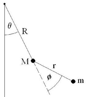
Figure 1: Notation for each of the double pendulums along the chain; see text for detail.

The second pendulum is not free to swingle through a full circle, but is instead constrained to stay in the range $|\phi^{a}_{i}|\leq\phi_{0}$. This constraint will also be modelled by adding a constraining potential, i.e. a potential $V_{c}(\phi)$ which has the effect of limiting de facto the excursion of the $\phi$ angles. The rest configuration will correspond to $\theta_{i}=\phi_{i}=0$.

Let us denote, dropping for a moment the index $i$, as $(X,Y)$ and $(x,y)$ the cartesian coordinates – in the plane orthogonal to the double helix axis $\xi$, with origin in the suspension point – of the point mass at the end of the first and of the second pendulum respectively. The vertical direction will be along the $x$ axis.

In the equilibrium position, given by $\theta=\phi=0$, we have $(X,Y)=(R,0)$ and $(x,y)=(R+r,0)$. In general, it will be

$$\begin{array}[]{ll}X=R\cos\theta\ ,&x=R\cos\theta+r\cos(\theta+\phi)\ ;\\ Y=R\sin\theta\ ,&y=R\sin\theta+r\sin(\theta+\phi)\ .\end{array}$$ (1)

The kinetical energy for the double pendulum at site $i$ will then be $T_{i}=(1/2)[M(({\dot{X}}_{i})^{2}+({\dot{Y}}_{i})^{2})+m(({\dot{x}}_{i})^{2}+({\dot{y}}_{i})^{2})]$; using (1) to express $X_{i},Y_{i}$ and $x_{i},y_{i}$ in terms of the angles $\theta_{i}$ and $\phi_{i}$, we get

$$\begin{array}[]{l}T_{i}\ =\ \frac{MR^{2}}{2}{\dot{\theta}}_{i}^{2}+\frac{m}{2}\left[R^{2}{\dot{\theta}}_{i}^{2}+2Rr\cos\phi_{i}\left(({\dot{\theta}}_{i})^{2}+{\dot{\theta}}_{i}{\dot{\phi}}_{i}\right)+r^{2}({\dot{\theta}}_{i}+{\dot{\phi}}_{i})^{2}\right]\ .\end{array}$$ (2)

The total kinetic energy is of course $T=\sum_{i}T_{i}$.

As for interactions, each pendulum will be coupled to nearest neighbors via harmonic potentials, i.e. linear springs attached to the $M$ and to the $m$ masses of the pendulums at sites $k$ and $k+1$. Moreover, the mass $m$ at the end of the second pendulums will experience a (site-independent) external potential.

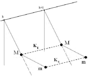
Figure 2: Pendulums at successive sites $k$ and $k+1$ interact via harmonic potentials coupling the masses at corresponding positions on the two pendulums; see text.

Thus we have the following forces, and correspondingly potential energy terms in the Lagrangian:

(1) A coupling between successive “first pendulums”, described by a potential

$$U_{t}^{(i)}\ =\ \kappa_{t}\,[1-\cos(\theta_{i+1}-\theta_{i})]\ ;$$ (3)

this will be referred to as the “torsional interaction”. The total torsional potential is of course $V_{t}=\sum_{a,i}U_{t}^{(a,i)}$.

(2) A coupling between successive “second pendulums” on each chain, described by a potential

$$U_{s}^{(i)}=(1/2)\kappa_{s}[(x_{i+1}-x_{i})^{2}+(y_{i+1}-y_{i})^{2}]\ ;$$

this will be referred to as “stacking interaction”. In terms of the $\theta_{i}$ and $\phi_{i}$ angles, using again (1) and with $\lambda=r/R$, we get

$$\begin{array}[]{rl}U_{s}^{(i)}=&(\kappa_{s}R^{2}/2)\,\left[\left((\cos\theta_{i}-\cos\theta_{i+1})+\lambda[\cos(\phi_{i}+\theta_{i})-\cos(\phi_{i+1}+\theta_{i+1})]\right)^{2}\right.\\ &\left.+\left((\sin\theta_{i}-\sin\theta_{i+1})+\lambda[\sin(\phi_{i}+\theta_{i})-\sin(\phi_{i+1}+\theta_{i+1})]\right)^{2}\right]\ ;\end{array}$$ (4)

the total stacking potential is of course $V_{s}=\sum_{a,i}V_{s}^{(a,i)}$.

(3) Interaction with the external potential,

$$U_{p}^{(i)}\ =\ F(\theta_{i},\phi_{i})\ .$$ (5)

The total external potential will of course be $V_{p}=\sum_{i}U_{p}^{(i)}$. In our case, the external potential will just be the gravitational one, i.e.

$$F(\theta_{i},\phi_{i})\ =\ g[MR(1-\cos\theta_{i})+m[R+r-(R\cos\theta_{i}+r\cos(\phi_{i}+\theta_{i}))]]\ .$$ (6)

(4) Interaction with the confining potential,

$$U_{c}^{(i)}\ =\ h(\phi_{i})\ ,$$ (7)

with $h(x)$ a convex even function, essentially flat for $|x|\ll\phi_{0}$, and rising sharply at $|x|\approx\phi_{0}$. The total external potential will of course be $V_{c}=\sum_{i}U_{c}^{(i)}$.

We have thus provided explicitly all terms appearing in the total Lagrangian

$$L\ =\ T\,-\,\left(U_{t}+U_{s}+U_{p}\right)\ .$$ (8)

The dynamics of the model will be governed by the corresponding Euler-Lagrange equations,

$$E_{\theta}\ := \ {\partial L\over\partial\theta_{i}}\,-\,{{\rm d}\ \over{\rm d}t}\left({\partial L\over\partial{\dot{\theta}}_{i}}\right)\ =\ 0\ ,$$

$$E_{\phi}\ := \ {\partial L\over\partial\phi_{i}}\,-\,{{\rm d}\ \over{\rm d}t}\left({\partial L\over\partial{\dot{\phi}}_{i}}\right)\ =\ 0\ .$$ (9)

We will not write these explicitly; they are rather involved, due mainly to the kinetic term.

3 Continuum version

If one is mainly interested in solutions varying little on the intersite scale, i.e. such that at all times $|\theta_{i+1}-\theta_{i}|$ and $|\phi_{i+1}-\phi_{i}|$ are small – say of order $\widehat{\varepsilon}\ll 1$, we can pass to a continuum description.

In this, the arrays $\theta_{i}(t)$ and $\phi_{i}(t)$ will be replaced by fields $\Theta(x,t)$ and $\Phi(x,t)$ such that, say, $\Phi(k\delta,t)=\phi_{k}(t)$ and $\Theta(k\delta,t)=\theta_{k}(t)$.

Expanding in a Taylor series up to order two in $\delta$ we have

$$\begin{array}[]{l}\Phi(x\pm\delta,t)=\Phi(x,t)\pm\delta\Phi_{x}(x,t)+(\delta^{2}/2)\Phi_{xx}(x,t)\ ,\\ \Theta(x\pm\delta,t)=\Theta(x,t)\pm\delta\Theta_{x}(x,t)+(\delta^{2}/2)\Theta_{xx}(x,t)\ .\end{array}$$ (10)

Inserting this into the Euler-Lagrange equations (2), we get the field equations, see (12) below, governing our system in the continuum approximation. In order to write these, it is convenient to set

$$\alpha(\Phi)\ :=\ 1+(R/r)\cos\Phi\ ,\ \ \beta(\Phi)\ :=\ (1+(R/r)^{2}+2(R/r)\cos\Phi)\;$$ (11)

we will moreover set

$$K_{s}\ :=\ \kappa_{s}\,\delta^{2}\ ,\ \ K_{t}\ :=\ \kappa_{t}\,\delta^{2}\ .$$

With these, we get the field equations

$$\begin{array}[]{l}\Theta_{xx}[K_{t}+K_{s}r^{2}\beta(\Phi)]+\Phi_{xx}[K_{s}r^{2}\alpha(\Phi)]\ =\\ \ =\ \Phi_{tt}[mr^{2}\alpha(\Phi)]+\Theta_{tt}[MR^{2}+mr^{2}\beta(\Phi)]+\\ \ \ -rR[m\Phi_{t}(\Phi_{t}+2\Theta_{t})-K_{s}\Phi_{x}(\Phi_{x}+2\Theta_{x})]\sin\Phi+\\ \ \ +g[R(m+M)\sin\Theta+mr\sin(\Phi+\Theta)]\ ;\\ K_{s}\Phi_{xx}r^{2}+\Theta_{xx}[K_{s}r^{2}\alpha(\Phi)]\ =\ m\Phi_{tt}r^{2}+\Theta_{tt}[mr^{2}\alpha(\Phi)]+\\ \ \ +h^{\prime}(\Phi)+rR(m\Theta_{t}^{2}-K_{s}\Theta_{x}^{2})\sin\Phi+gmr\sin(\Phi+\Theta)\ .\end{array}$$ (12)

We will from now on work in the continuum approximation, i.e. with (12).

These are also obtained by rewriting the Lagrangian $L$ in the continuum approximation; the explicit expression of this (written for future reference) is

$$\begin{array}[]{l}{\mathcal{L}}=(1/2)\left[MR^{2}\Theta_{t}^{2}-K_{t}\Theta_{x}^{2}+m\left(r^{2}(\Phi_{t}+\Theta_{t})^{2}+R^{2}\Theta_{t}^{2}\right.\right.\\ \left.\left.+2rR\Theta_{t}(\Phi_{t}+\Theta_{t})\cos\Phi\right)\right.\\ \left.+2g[(m+M)R\cos\Theta+mr\cos(\Phi+\Theta)]-2h[\Phi]\right.\\ \left.-K_{s}[\left(R\Theta_{x}\cos\Theta+r(\Phi_{x}+\Theta_{x})\cos(\Phi+\Theta)\right)^{2}\right.\\ \left.+\left(R\Theta_{x}\sin\Theta+r(\Phi_{x}+\Theta_{x})\sin(\Phi+\Theta)\right)^{2}]\right]\ .\end{array}$$ (13)

Then (12) are also obtained as the associate Euler-Lagrange equations

$$\mathcal{E}_{\Theta} := {\partial{\mathcal{L}}\over\partial\Theta}\,-\,{{\rm d}\ \over{\rm d}t}\left({\partial{\mathcal{L}}\over\partial\Theta_{t}}\right)\,-\,{{\rm d}\ \over{\rm d}x}\left({\partial{\mathcal{L}}\over\partial\Theta_{x}}\right)\ =\ 0\ ,$$

$$\mathcal{E}_{\Phi} := {\partial{\mathcal{L}}\over\partial\Phi}\,-\,{{\rm d}\ \over{\rm d}t}\left({\partial{\mathcal{L}}\over\partial\Phi_{t}}\right)\,-\,{{\rm d}\ \over{\rm d}x}\left({\partial{\mathcal{L}}\over\partial\Phi_{x}}\right)\ =\ 0\ .$$ (14)

The field equations (12) should be supplemented by a specification of the function space the solution are required to belong to; these can be given as boundary conditions.

The physically natural condition is that of finite energy at any time $t$; that is, considering the energy density

$$H(x,t)\ =\ H[\Theta(x,t),\Phi(x,t)]\ =\ T+(U_{t}+U_{s}+U_{p}+U_{c})\ ,$$ (15)

and fixing the additive arbitrary constant so that the minimum of the potential energy is at zero, the requirement that

$$\int_{-\infty}^{+\infty}H(x,t)\,{\rm d}x\ <\ \infty.$$ (16)

For this to be satisfied, in view of the form of $T$, we must require that

$$\lim_{x\to\pm\infty}\Phi_{x}\ =\ \lim_{x\to\pm\infty}\Theta_{x}\ =\ 0\ ,$$ (17)

i.e. that $\Phi$ and $\Theta$ are asymptotically constant in $x$.

Moreover, the fields $\Phi$ and $\Theta$ should go at minima of the potential energy for $x\to\pm\infty$; in view of the form of the potential energy, we must actually require that

$$\lim_{x\to\pm\infty}\Phi\ =\ 0\ ;\ \lim_{x\to\pm\infty}\Theta\ =\ 2\pi n_{\pm}\ .$$ (18)

(Note that the difference between topological and non topological degrees of freedom shows up here.)

We can always change origin of the $\Theta$ angles, so that

$$\lim_{x\to-\infty}\Theta=0\ ,\ \lim_{x\to+\infty}\Theta=2\pi N\ .$$ (19)

Thus, finite energy solutions possess a topological index, the integer $N$, identified by the asymptotic behavior at $x\to\pm\infty$. One gets easily convinced that these boundary conditions (and the finite energy condition) are preserved under the time evolution described by (12).

4 Travelling wave solutions

We are specially interested in travelling wave (TW) solutions, i.e. solutions such that

$$\Theta(x,t)=\vartheta(x-vt)\equiv\vartheta(z),\ \Phi(x,t)=\varphi(x-vt)\equiv\varphi(z)\ .$$ (20)

It is immediate to see that the boundary conditions implied by the requirement of finite energy become in this framework

$$\begin{array}[]{ll}\lim_{z\to\pm\infty}\varphi^{\prime}(z)=0\ ,&\lim_{z\to\pm\infty}\vartheta^{\prime}(z)=0\ ;\\ \lim_{z\to\pm\infty}\varphi(z)=0\ ,&\lim_{z\to\pm\infty}\vartheta(z)=2\pi n_{\pm}\ .\end{array}$$ (21)

We will again choose variables so that $\vartheta(-\infty)=0$, $\vartheta(+\infty)=2\pi N$.

Inserting the ansatz (20) into the equations (12), and writing $M=\rho m$ for ease of notation, we get the equations for travelling wave solutions:

$$\begin{array}[]{l}\mu\varphi_{zz}(r^{2}+rR\cos\varphi)+\vartheta_{zz}[K_{t}-K_{s}R^{2}\rho+\mu(r^{2}+R^{2}+R^{2}\rho+2rR\cos\varphi)]+\\ \ \ -\mu rR\varphi_{z}^{2}\sin\varphi-2\mu rR\varphi_{z}\vartheta_{z}\sin\varphi-mg[R(1+\rho)\sin\vartheta+r\sin(\varphi+\vartheta)]\ =\ 0\ ;\\ {}\\ \mu r^{2}\varphi_{zz}+\mu\vartheta_{zz}r(r+R\cos\varphi)-h^{\prime}(\varphi)+\mu rR\vartheta_{z}^{2}\sin\varphi-mgr\sin(\varphi+\vartheta)\ =\ 0\ .\end{array}$$ (22)

Here we have simplified the writing by defining the parameter

$$\mu\ :=\ K_{s}-mv^{2}\ ;$$ (23)

this will have a relevant role in the following.

In the following it will be of interest to consider the Lagrangian ${\mathcal{L}}_{tw}$ producing the travelling wave equations (22) as associated Euler-Lagrange equations; this is also obtained by restricting the Lagrangian (13) to the space of functions satisfying (20). It results

$$\begin{array}[]{ll}{\mathcal{L}}_{tw}\ =&(1/2)\left[mr^{2}\beta(\varphi)v^{2}+MR^{2}v^{2}-K_{t}\right.\\ &\left.\ \ \ -K_{s}r^{2}\beta(\varphi)\right]\,\vartheta_{z}^{2}\ +\ (1/2)\left[r^{2}(mv^{2}-K_{s})\right]\,\varphi_{z}^{2}\\ &\ +\left[(mv^{2}-K_{s})r^{2}\alpha(\varphi)\right]\,\vartheta_{z}\varphi_{z}\\ &\ +\left[\left((m+M)gR\cos\vartheta+mgr\cos(\varphi+\vartheta)\right)+h(\varphi)\right]\ .\end{array}$$ (24)

5 Series expansion for TW solutions

A way to obtain the simple pendulums chain (and the sine-Gordon equation in the continuum limit) from our model is to let the length of second pendulums go to zero. Note that in this case our set of parameters becomes redundant, as the masses $m$ and $M$ coincide in space, so that only the total mass $\widehat{M}=m+M$ is relevant; and similarly for the coupling constants $K_{s}$ and $K_{t}$, with total coupling strength $\widehat{K}=K_{s}+K_{t}$.

If the double pendulums chain is seen as a (singular) perturbation of the simple pendulums one, one is naturally led to look for travelling wave solutions as perturbations of the standard sine-Gordon solitons.

We will thus now look for solutions to the (22) equations in the form of a series expansion in a small parameter $\varepsilon$,

$$\begin{array}[]{l}\vartheta\ =\ \vartheta_{0}+\varepsilon\vartheta_{1}+\varepsilon^{2}\vartheta_{2}+....\ ,\\ \varphi\ =\ \varphi_{0}+\varepsilon\varphi_{1}+\varepsilon^{2}\varphi_{2}+....\ .\end{array}$$ (25)

We will correspondingly also expand in the same parameter the geometrical parameters and the masses appearing in our model, and also allow for modification of the speed by expanding it as well:

$$\begin{array}[]{l}r\ =\ r_{0}+\varepsilon r_{1}+\varepsilon^{2}r_{2}+...\ ,\\ R\ =\ A-r_{0}-\varepsilon r_{1}-\varepsilon^{2}r_{2}-...\ ;\\ m\ =\ m_{0}+\varepsilon m_{1}+\varepsilon^{2}m_{2}+...\ ,\\ M\ =\ {\widehat{M}}-m_{0}-\varepsilon m_{1}-\varepsilon^{2}m_{2}-...\ ;\\ v\ =\ v_{0}+\varepsilon v_{1}+\varepsilon^{2}v_{2}+...\ ;\end{array}$$ (26)

note that $A$ and ${\widehat{M}}$ represent the total length and total mass of each double pendulum in the chain, which are kept constant as $\varepsilon$ is varied. In other words, we are now rescaling the model with $\varepsilon$.

We would like this is done so that for $\varepsilon\to 0$ the double pendulums chain reduces to a simple pendulums chain, with same total length $A$ and total mass ${\widehat{M}}$; this requires $r_{0}=0$. The choice of $m_{0}$ is at this point inessential (in the limit we have a single pendulum with mass ${\widehat{M}}=M+m$), but for the sake of simplicity we will choose $m_{0}=0$.

It should also be noted that once the double pendulum reduces to a simple one, the presence of two coupling constants $K_{t}$ and $K_{s}$ is actually redundant, as they intervene (in the limit, i.e. for $\varepsilon\to 0$) exactly in the same interaction: only $K:=K_{s}+K_{t}$ is relevant. Thus we will also write

$$\begin{array}[]{l}K_{t}\ =\ \varepsilon k_{1}+\varepsilon^{2}k_{2}+...\ ,\\ K_{s}\ =\ \widehat{K}\,-\varepsilon k_{1}-\varepsilon^{2}k_{2}-...\ .\end{array}$$ (27)

Finally, we note that for $\varepsilon\to 0$ and hence for the single pendulums chain, the angle $\varphi$ makes no sense; in order to avoid any paradoxical behavior, we would require that it gets frozen to zero for $\varepsilon\ll 1$, i.e.

$$\varphi_{0}\ =\ 0\ .$$ (28)

Summarizing our discussion, the series expansion we adopt are as follows:

$$\begin{array}[]{lll}\vartheta&=\ \vartheta_{0}+\varepsilon(\delta\theta)&=\ \vartheta_{0}+\varepsilon\vartheta_{1}+\varepsilon^{2}\vartheta_{2}+....\ ,\\ \varphi&=\ \varepsilon(\delta\varphi)&=\ \varepsilon\varphi_{1}+\varepsilon^{2}\varphi_{2}+....\ ;\\ r&=\ \varepsilon(\delta r)&=\ \varepsilon r_{1}+\varepsilon^{2}r_{2}+...\ ,\\ R&=\ A-\varepsilon(\delta r)&=\ A-\varepsilon r_{1}-\varepsilon^{2}r_{2}-...\ ;\\ m&=\ \varepsilon(\delta m)&=\ \varepsilon m_{1}+\varepsilon^{2}m_{2}+...\ ,\\ M&=\ {\widehat{M}}-\varepsilon(\delta m)&=\ {\widehat{M}}-m_{0}-\varepsilon m_{1}-\varepsilon^{2}m_{2}-...\ ;\\ v&=\ v_{0}+\varepsilon(\delta v)&=\ v_{0}+\varepsilon v_{1}+\varepsilon^{2}v_{2}+...\ ;\\ K_{t}&=\ \varepsilon(\delta\widehat{K})&=\ \varepsilon k_{1}+\varepsilon^{2}k_{2}+...\ ,\\ K_{s}&=\ \widehat{K}-\varepsilon(\delta\widehat{K})&=\ \widehat{K}\,-\varepsilon k_{1}-\varepsilon^{2}k_{2}-...\ .\end{array}$$ (29)

We will then insert the series expansions (29) in the Euler-Lagrange equations for TW solutions (22). It will be convenient to define

$$\widehat{\mu}\ :=\ (\widehat{M}\,v_{0}^{2}\ -\ \widehat{K})\ .$$ (30)

5.1 Terms of order zero

At order zero, the second equation in (22) is identically satisfied (it just reduces to $h^{\prime}(0)=0$, which always holds for $h$ even), while the first reads

$${\vartheta_{0}}^{\prime\prime}\ =\ -{\widehat{M}g\over A\widehat{\mu}}\ \sin(\vartheta_{0})\ :=\ -\,\kappa\ \sin(\vartheta_{0})\ .$$ (31)

This reproduces – as obvious by construction – the sine-Gordon equations for the single pendulums chain. Its solution is

$$\vartheta_{0}(z)\ =\ 4\ \arctan\left[\exp(\kappa\,z)\right]\ .$$ (32)

Derivatives of this function are readily computed, and we have

$$\vartheta_{0}^{\prime}\ =\ 2{\kappa\over\cosh(\kappa z)}\ ,\ \ {\vartheta_{0}}^{\prime\prime}\ =\ -\,2\ {\kappa^{2}\ \sinh(\kappa^{2}z)\over\cosh^{2}(\kappa^{2}z)}\ .$$ (33)

These will appear in the higher order term of the expansion of (22); in these we also find terms like $\sin(\vartheta_{0})$ and $\cos(\vartheta_{0})$, which in view of (32) – and with some simple algebra – are given by

$$\sin(\vartheta_{0})\ =\ -2\,{\sinh(\kappa x)\over\cosh^{2}(\kappa x)}\ ,\ \ \cos(\vartheta_{0})\ =\ {\sinh^{2}(\kappa x)-1\over\cosh^{2}(\kappa x)}\ .$$ (34)

5.2 Terms of order one

At order $\varepsilon$, and using the equation at order $\varepsilon^{0}$, the first of (22) reads

$$\begin{array}[]{l}{\vartheta_{1}}^{\prime\prime}\ =\ \ [A^{2}\widehat{\mu}]^{-1}\ \left[\left((A^{2}-1)k_{1}+2A\widehat{M}v_{0}(Av_{1}-r_{1}v_{0})\right){\vartheta_{0}}^{\prime\prime}+\right.\\ \left.\ \ +(A\widehat{M}g\cos\vartheta_{0})\vartheta_{1}-\widehat{M}gr_{1}\sin\vartheta_{0}\right]\ .\end{array}$$ (35)

Using the solution for $\vartheta_{0}$ and its consequences recalled above, this simplifies to

$$\begin{array}[]{ll}{\vartheta_{1}}^{\prime\prime}\ =&-\,\left(\widehat{M}^{2}g^{2}{\rm sech}^{2}(\kappa z)\,/\,(2A^{5}\widehat{K}^{2})\right)\ \times\\ &\times\left[A^{3}\widehat{K}\left(\cosh(2\kappa z)-3\right)\,\vartheta_{1}\ +\ 4\,B\,\,\sinh(\kappa z)\right]\ ,\end{array}$$ (36)

where we have written

$$B\ :=\ \left(A^{2}\kappa r_{1}-\widehat{M}g((1-A^{2})k_{1}+2A\widehat{M}v_{0}(r_{1}v_{0}-Av_{1}))\right)\ .$$ (37)

As for the order $\varepsilon$ terms in the second of (22), these yield

$$\varphi_{1}\ =\ {\widehat{M}g\widehat{K}r_{1}\over\widehat{\mu}\,h^{\prime\prime}(0)}\ \sinh(\vartheta_{0})\ .$$ (38)

It should be stressed that these two equations, (36) and (38), are qualitatively different: in facts, while the first is a (second order) differential equation for $\vartheta_{1}$, which depends on $\vartheta_{0}$, the second is an algebraic identity which directly determines $\varphi_{1}$.

5.3 Higher order terms

Proceeding with the analysis at higher and higher orders, we would of course obtain more and more involved explicit equations. However, the main feature displayed at order one will be present at higher orders $k>1$ as well.

That is $\vartheta_{k}$ will be determined by a differential equation of the form

$${\vartheta_{k}}^{\prime\prime}\ =\ F_{k}[\vartheta_{0},...,\vartheta_{k-1};\varphi_{1},...,\varphi_{k-1}]\,\vartheta_{k}\ +\ G_{k}[\vartheta_{0},...,\vartheta_{k-1};\varphi_{1},...,\varphi_{k-1}]\$$

(omitting for the sake of brevity the dependence on parameters).

This can be seen as the equation of motion for a particle of unit mass, whose position is described by $\vartheta_{k}(t)$, in the time-dependent potential

$$V_{k}(\vartheta_{k},t)\ :=\ -(1/2)\widetilde{F}_{k}(t)(\vartheta_{k})^{2}\ -\ \widetilde{G}_{k}(t)(\vartheta_{k})\ ,$$ (39)

where we have used the fact $\vartheta_{j}(t)$, $\varphi_{j}(t)$ with $j<k$ can be determined by solving equations at lower orders so to write

$$\widetilde{F}_{k}(t)\ :=\ F_{k}[\vartheta_{0}(t),...,\vartheta_{k-1}(t);\varphi_{1}(t),...,\varphi_{k-1}(t)]\ .$$ (40)

As for the term $\varphi_{k}$, this will not be determined by a differential equation, but rather by an algebraic relation, i.e.

$$\varphi_{k}\ =\ H_{k}[\vartheta_{0},...,\vartheta_{k-1};\varphi_{1},...,\varphi_{k-1}]\ .$$ (41)

E.g., at order $\varepsilon^{2}$, and using the results from the analysis of terms of order $\varepsilon^{0}$ and $\varepsilon^{1}$, we get for this algebraic relation

$$\begin{array}[]{l}\varphi_{2}=[g/(2A^{2}\widehat{\mu}^{2}h^{\prime\prime}(0))]\times\\ \ \times\left[A^{2}K\widehat{M}r_{1}{\rm sech}^{2}(\kappa z)(\cos(2\kappa z)-3)(h^{\prime\prime}(0))^{2}\vartheta_{1}\right.\\ \ \left.+\ 4K\widehat{M}r_{1}[k_{1}-A^{2}k_{1}+A(\widehat{\mu}r_{1}+2\widehat{M}v_{0}(r_{1}v_{0}-Av_{1}))]\times\right.\\ \ \left.\times{\rm sech}(\kappa z)\tanh(\kappa z)(h^{\prime\prime}(0))^{2}\right.\\ \ \left.+\ A^{2}\sin(\vartheta_{0})[-2\widehat{\mu}h^{\prime\prime}(0)(-AK^{2}\widehat{M}r_{1}^{2}(\vartheta_{1}^{\prime})^{2}\right.\\ \ \left.+\ (k_{1}\widehat{M}r_{1}-K\widehat{M}r_{2}+m_{1}r_{1}(\widehat{\mu}+\widehat{M}v_{0}^{2}))h^{\prime\prime}(0))\right.\\ \ \left.-\ gK^{2}\widehat{M}^{2}r_{1}^{2}\sin(\vartheta_{0})h^{\prime\prime\prime}(0)]\right]\ .\end{array}$$ (42)

It should be noted that the algebraic – rather than differential – character of the relation (41) is due, in algebraic terms, to the choice $r_{0}=0$ (which also means we are considering a singular perturbation [16]). This makes that the terms with derivatives of $\varphi_{k}$ will not appear in the $O(\varepsilon^{k})$ terms of the expansion, while $\varphi_{k}$ itself does; hence we have an algebraic relation and not a differential equation.

In physical terms, the choice $r_{0}=0$ corresponds indeed to considering the double pendulums chain as a perturbation of the single pendulums one, the perturbation parameter being related to the length of second pendulums.

In facts, let us substitute according to the condensate form of (29) into (24): we write the resulting expansion as

$${\mathcal{L}}_{tw}\ =\ {\mathcal{L}}_{0}\ +\ \varepsilon\,{\mathcal{L}}_{1}\ +\ \varepsilon^{2}\,{\mathcal{L}}_{2}\ +\ O(\varepsilon^{3})\ .$$ (43)

We will not set $\varphi_{0}\equiv 0$. At first orders we have the expressions reported in Appendix B

The complete explicit form of these is not so relevant; the important fact is that – as can be checked explicitly by the formulas in Appendix B – we have

$$\partial{\mathcal{L}}_{k}/\partial\varphi_{k}^{\prime}\ =\ 0\ ;$$ (44)

hence the corresponding Euler-Lagrange equation (no sum on $k$ here and below)

$${\partial{\mathcal{L}}_{k}\over\partial\varphi_{k}}\ -\ {d\over dt}{\partial{\mathcal{L}}_{k}\over\partial\varphi_{k}^{\prime}}\ =\ 0$$ (45)

reduces to the identity

$${\mathcal{A}}_{k}\ :=\ \ {\partial{\mathcal{L}}_{k}\over\partial\varphi_{k}}\ =\ 0\ .$$ (46)

These equations show that – as anticipated in the Introduction – to any order of the perturbative expansion the Lagrangian ${\mathcal{L}}_{k}$ depends on $\varphi_{k}$ but is independent of the momentum conjugated to $\varphi_{k}$: that is, the $\varphi_{k}$ can be considered as an auxiliary field, entering in the Lagrangian only algebraically (and not differentially). We express this fact by saying that the field $\varphi$ is a perturbatively auxiliary field. We stress that $\varphi$ is not an auxiliary field in the full Lagrangian, i.e. its auxiliary character arises as a consequence of the (singular) perturbative expansion we considered.

In facts, the above explicit expressions for ${\mathcal{L}}_{0},{\mathcal{L}}_{1},{\mathcal{L}}_{2}$ provide the expression for the first few identities ${\mathcal{A}}_{k}$, which all reduce to $h^{\prime}(\varphi_{0})=0$.

If we look at the Euler-Lagrange equations

$${\mathcal{E}}_{k,j}\ :=\ {\partial{\mathcal{L}}_{k}\over\partial\varphi_{k-j}}\ -\ {d\over dt}{\partial{\mathcal{L}}_{k}\over\partial\varphi_{k-j}^{\prime}}\ =\ 0\ ,$$ (47)

these reduce to the algebraic identities seen above.

In particular, we have

$${\mathcal{E}}_{1,0} = AKr_{1}(\vartheta_{0}^{\prime\prime}\cos\varphi_{0}+2(\vartheta_{0}^{\prime})^{2}\sin\varphi_{0})+\varphi_{1}h^{\prime\prime}(\varphi_{0})=0\ ;$$

$${\mathcal{E}}_{2,1} = AKr_{1}(\vartheta_{0}^{\prime\prime}\cos\varphi_{0}+2(\vartheta_{0}^{\prime})^{2}\sin\varphi_{0})+\varphi_{1}h^{\prime\prime}(\varphi_{0})=0\ ;$$

$${\mathcal{E}}_{2,0} = [-Kr_{1}^{2}\vartheta_{0}^{\prime\prime}+A(K(2\varphi_{1}r_{1}(\vartheta_{0}^{\prime})^{2}+r_{2}\vartheta_{0}^{\prime\prime}+r_{1}\vartheta_{1}^{\prime\prime})$$

$$\ \ \ -r_{1}(k_{1}+m_{1}v_{0}^{2})\vartheta_{0}^{\prime\prime})]\cos\varphi_{0}$$

$$-[2Kr_{1}^{2}(\vartheta_{0}^{\prime})^{2}+A(2k_{1}r_{1}(\vartheta_{0}^{\prime})^{2}-2Kr_{2}(\vartheta_{0}^{\prime})^{2}+Kr_{1}\varphi_{1}\vartheta_{0}^{\prime\prime}-4Kr_{1}\vartheta_{0}^{\prime}\vartheta_{1}^{\prime}$$

$$\ \ \ +2m_{1}r_{1}v_{0}^{2}(\vartheta_{0}^{\prime})^{2})]\sin\varphi_{0}$$

$$+r_{1}(Kr_{1}(2\varphi_{0}^{\prime\prime}+\vartheta_{0}^{\prime\prime})-gm_{1}\sin(\varphi_{0}+\vartheta_{0}))+(1/2)\varphi_{1}^{2}h^{\prime\prime\prime}(\varphi_{0})$$

$$+h^{\prime\prime}(\varphi_{0})\,\varphi_{2}\ =\ 0\ .$$

6 Discussion and conclusions

We have considered a model corresponding to a chain of double pendulums (with a constraining potential limiting excursions of second pendulums), with first-neighbor harmonic interactions and possibly subject to an external potential. This can, in an appropriate limit, be considered as a perturbation of the usual simple pendulums chain with harmonic interactions, possibly subject to an external potential, leading to (discrete) sine-Gordon solitons.

We dealt with these models in the continuum limit; in this case the field equations we obtain describe two interacting fields (possibly in an external potential) a topological field $\Theta(x,t)$ and a non-topological one $\Phi(x,t)$.

Looking for travelling wave solutions – which include in particular simple solitons – with velocity $v$, we obtain a reduction to two coupled second order ODEs for $\vartheta(z)$ and $\varphi(z)$, where $z=(x-vt)$.

These equations posses a Hamiltonian structure and as such they can be studied using conservation of energy; this reduces the effective dynamics – for given initial data – to a three dimensional manifold. However, the lack of a second constant of motion prevents integrability and hence obtaining a general solution for the dynamics.

We argued then that our model can be seen, as mentioned above, as a perturbation of the standard simple pendulums model leading in the continuum approximation to sine-Gordon equations. The perturbation parameter $\varepsilon$ should lead not only field expansion, but also appropriate expansions for the geometrical and dynamical parameters of the model. We would thus expect that – for small $\varepsilon$ – the solitons of our model can be expressed as perturbations of the familiar sine-Gordon solitons.

By performing explicitly the perturbative expansion and solving the resulting equation at first order, we have shown that this is the case. However, in this procedure we obtained a rather unexpected feature: that is, the non-topological field is determined by the topological one via an algebraic relation – not a differential equation – and thus has the role of a slaved field, while the topological field takes the role of master field.

This feature is due to the appearance of a perturbatively auxiliary field; that is, when we expand perturbatively our model around the $\vartheta_{0}$ soliton, the field $\varphi=\varepsilon\varphi_{1}+\varepsilon^{2}\varphi_{2}+...$ is an auxiliary field, determined by algebraic equations, up to any desired order – but it is not an auxiliary field for the full dynamics.

We have already noted (see appendix A for details) that the simple pendulum system can be also obtained, acting on the confining potential, as a dynamical limit of the double pendulums chain. Thus, the double pendulums chain can be reduced to a single pendulums chain in two conceptually (and physically) independent ways: the dynamical way discussed in Ref. [11] and the singular limit discussed in this paper. Although leading to the same simple physical system, the two different reductions have peculiar features that make them rather different. Therefore they may be used in different contexts to model the dynamics of realistic systems such as molecular chains.

The most striking difference between the two simple pendulums reductions is related to the breaking of boost (Lorentz) symmetry. Owing to the presence of two different sound speeds (related to the presence of two coupling constants $K_{t},K_{s}$), the lagrangian (13) is not invariant under Lorentz transformation [11]. However, performing the $\varepsilon\to 0$ limit, at the zeroth order in the perturbation theory we recover Lorentz invariance and the speed of the sine-Gordon soliton is not fixed. The recovering of the boost symmetry is essentially a consequence of the fact that in the limit $\varepsilon\to 0$ only the coupling $K=K_{s}+K_{t}$ and the mass $\hat{M}=m+M$ (not the single couplings or single masses) are relevant. It follows that in this limit we have just one (and not two) speed of sound $\sqrt{K/\hat{M}}$. Obviously, the boost symmetry is broken by higher orders in the perturbative $\varepsilon$-expansion, but perturbative solution can be still found for any value of the speed of the travelling wave. Conversely, in the case of the dynamical single pendulum reduction the Lorentz symmetry remains broken also after the reduction and the soliton speed is fixed (see appendix A). Moreover, in this later case it is very difficult to find perturbative solutions of the double pendulums chain and one has to resort to numerical calculations [1].

In conclusion, the dynamical reduction to a single pendulums chain provide us with a nice mechanism to fix the speed of sine-Gordon solitons, can be applied in presence of a strong confining potential but is not suitable for a perturbative evaluation of the solutions of the double pendulums model. On the other hand, the singular $\varepsilon$-expansion discussed in this paper provide us with a nice perturbative framework for evaluating the general solutions of the model, can be applied in presence of weak confining potentials but does not allow for a soliton speed fixing mechanism.

Appendix A.
The dynamical simple pendulums limit

Now we note that if we force $\Phi(x,t)=0$ – and hence $\varphi(z)=0$ – in our model, then we are actually considering a chain of simple pendulums; in the continuum limit, this leads to a sine-Gordon equation.

The constraint $\Phi(x,t)=0$ can be accommodated, in our setting, by acting on the confining potential $U_{c}$, i.e. on $h$: this should be made stronger and stronger – hence we speak of a dynamical limit, as opposed to the geometrical one considered above – and the maximum angle $\phi_{0}$ smaller and smaller.

In the limit $\phi_{0}\to 0^{+}$ and $h^{\prime\prime}(0)\to+\infty$, we expect to recover the solitons of the sine-Gordon equation. Note that in this limit the coupling constants $K_{s}$ and $K_{t}$ actually refer to the same interaction; we will thus take $K_{t}=0$, also in order to make comparison with the sine-Gordon case more immediate.

If we force $\varphi(z)\equiv 0$, and use $h^{\prime}(0)=0$, $K_{t}=0$, then the equations (22) reduce to

$$\begin{array}[]{l}[\mu(2rR+r^{2}+R^{2}(1+\rho))-K_{s}R^{2}\rho]\vartheta_{zz}+gm(r+R+R\rho)\sin\vartheta\ =\ 0\ ;\\ \mu r(r+R)\vartheta_{zz}+gmr\sin\vartheta\ =\ 0\ .\end{array}$$

Each of these two equations provide a different determination for $\vartheta_{zz}$; the compatibility condition for them is obtained requiring the two determinations coincide. When $r\not=0$ (if $r=0$ the second equation is identically satisfied) the compatibility condition reads

$$\mu\ =\ -K_{s}R/r\ .$$

This provides a unique determination for $\mu$ and hence, in view of (23), for $v^{2}$; more precisely, this yields

$$v\ =\ \pm\ \sqrt{{K_{s}(r+R)\over mr}}\ .$$

Thus, the compatibility condition selects uniquely the speed of the travelling wave obtained in the dynamical simple pendulums limit.

This phenomenon is not peculiar to our model, but common to a large class of multi-fields soliton models, as discussed elsewhere [11].

Appendix B.
Expansion of the travelling wave Lagrangian

In this Appendix we provide explicit formulas for the first terms in the perturbative expansion (43) of the travelling wave Lagrangian (24). These are:

$$\begin{array}[]{l}{\mathcal{L}}_{0}=(A/2)\left[A(\widehat{M}v_{0}^{2}-K)(\vartheta_{0}^{\prime})^{2}-2g\widehat{M}\cos\vartheta_{0}-2h(0)\right]\ ;\\ {}\\ {\mathcal{L}}_{1}=\left[(1/2)(A^{2}-1)k_{1}+Ar_{1}(K-\widehat{M}v_{0}^{2})+A^{2}\widehat{M}v_{0}v_{1}-AKr_{1}\cos\varphi_{0}\right](\vartheta_{0}^{\prime})^{2}\\ \ -\ A^{2}(K-\widehat{M}v_{0}^{2})(\vartheta_{0}^{\prime}\vartheta_{1}^{\prime})-\ AKr_{1}\cos\varphi_{0}(\vartheta_{0}^{\prime}\varphi_{0}^{\prime})\\ \ -\ g\widehat{M}(a\vartheta_{1}\sin\vartheta_{0}-r_{1}\cos\vartheta_{0})\vartheta_{0}^{\prime}\ -\ [h^{\prime}(\varphi_{0})]\varphi_{1}\ ;\\ {}\\ {\mathcal{L}}_{2}=(A^{2}/2)(\widehat{M}v_{0}^{2}-K)(\vartheta_{1}^{\prime})^{2}-(1/2)Kr_{1}^{2}(\varphi_{0}^{\prime})^{2}-AKr_{1}\cos\varphi_{0}(\varphi_{0}^{\prime}\vartheta_{1}^{\prime})\\ \ +(1/2)[(A^{2}-1)k_{2}-2r_{1}(Ak_{1}-Kr_{1})+2AKr_{2}+\widehat{M}r_{1}^{2}v_{0}^{2}-2A\widehat{M}r_{2}v_{0}^{2}\\ \ -4A\widehat{M}r_{1}v_{0}v_{1}+A^{2}\widehat{M}v_{1}^{2}+2A^{2}\widehat{M}v_{0}v_{2}\\ \ \ +2(Ak_{1}r_{1}+Kr_{1}^{2}-2AKr_{2}+2Am_{1}r_{1}v_{0}^{2})\cos\varphi_{0}+2AKr_{1}\varphi_{1}\sin\varphi_{0}](\vartheta_{0}^{\prime})^{2}\\ \ +\widehat{M}gr_{2}\cos\vartheta_{0}+(1/2)Ag\widehat{M}\vartheta_{1}^{2}\cos\vartheta_{0}-gm_{1}r_{1}\cos(\varphi_{0}+\vartheta_{0})\\ \ -g\widehat{M}(r_{1}\vartheta_{1}-A\vartheta_{2})\sin\vartheta_{0}-\varphi_{2}h^{\prime}(\varphi_{0})-(1/2)\varphi_{1}^{2}h^{\prime\prime}(\varphi_{0})\\ \ \ +[A^{2}(\widehat{M}v_{0}^{2}-K)\vartheta_{2}^{\prime}+((A^{2}-1)k_{1}+2AKr_{1}-2A\widehat{M}r_{1}v_{0}^{2}+2A^{2}\widehat{M}v_{0}v_{1}\\ \ \ \ -2AKr_{1}\cos\varphi_{0})\vartheta_{1}^{\prime}\ +\ ((AK_{1}r_{1}+Kr_{1}^{2}-AKr_{2}+Am_{1}r_{1}v_{0}^{2})\cos\varphi_{0}\\ \ \ +AKr_{1}\varphi_{1}\sin\varphi_{0}-Kr_{1}^{2})]\vartheta_{0}^{\prime}\ .\end{array}$$

These expressions allow to check explicitly (at first orders) that (44) holds, and hence (45) reduce to (46).

References

- [1] M. Cadoni, R. De Leo and G. Gaeta, “A composite model for DNA torsion dynamics”, Phys. Rev. E 75, 021919 (2007).
- [2] M. Peyrard and A.R. Bishop, “Statistical mechanics of a nonlinear model for DNA denaturation”, Phys. Rev. Lett. 62 (1989), 2755-2758
- [3] L.V. Yakushevich, “Nonlinear DNA dynamics: a new model”, Phys. Lett. A 136 (1989), 413-417
- [4] G. Gaeta, C. Reiss, M. Peyrard and Th. Dauxois, “Simple models of non-linear DNA dynamics”, Rivista del Nuovo Cimento 17 (1994) n.4, 1–48
- [5] L.V. Yakushevich, Nonlinear Physics of DNA, Wiley (Chichester) 1998; second edition 2004
- [6] M. Barbi, S. Cocco and M. Peyrard, “Helicoidal model for DNA opening”, Phys. Lett. A 253 (1999), 358-369; “Vector nonlinear Klein-Gordon lattices: general derivation of small amplitude envelope soliton solution”, Phys. Lett. A 253 (1999), 161-167
- [7] M. Barbi, S. Cocco, M. Peyrard and S. Ruffo, “A twist-opening model of DNA”, J. Biol. Phys. 24 (1999), 97-114
- [8] S. Cocco and R. Monasson, “Statistical mechanics of torque induced denaturation of DNA”, Phys. Rev. Lett. 83 (1999), 5178-5181
- [9] M. Peyrard and Th. Dauxois, “Physique des solitons”, Editions du CNRS (Paris) 2004; “Physics of Solitons”, Cambridge University Press 2006
- [10] M. Peyrard, “Nonlinear dynamics and statistical physics of DNA”, Nonlinearity 17 (2004) R1-R40
- [11] M. Cadoni, R. De Leo and G. Gaeta, “A symmetry breaking mechanism for selecting the speed of relativistic solitons”, to appear in J. Phys. A
- [12] L. Venier, “Onde solitarie nei modelli della catena del DNA”, M.Sc. Thesis, Dipartimento di Matematica, Università di Milano, 2007; G. Gaeta and L. Venier, “Solitary waves in helicoidal models of DNA dynamics”, forthcoming paper.
- [13] J. Wess and J. Bagger, Supersymmetry and supergravity, Princeton University Press, Princeton, New Jersey, 1983.
- [14] P. Van Nieuwenhuizen, “Supergravity”, Phys. Rep. 68,(1981) 189-398
- [15] S.W. Englander, N.R. Kallenbach, A.J. Heeger, J.A. Krumhansl and A. Litwin, “Nature of the open state in long polynucleotide double helices: possibility of soliton excitations”, PNAS USA 77 (1980), 7222-7226
- [16] F. Verhulst, “Methods and applications of singular perturbations”, Springer (Berlin) 2005