Dynamics of DNA-breathing: Weak noise analysis, finite time singularity, and mapping onto the quantum Coulomb problem

Abstract

We study the dynamics of denaturation bubbles in double-stranded DNA on the basis of the Poland-Scheraga model. We show that long time distributions for the survival of DNA bubbles and the size autocorrelation function can be derived from an asymptotic weak noise approach. In particular, below the melting temperature the bubble closure corresponds to a noisy finite time singularity. We demonstrate that the associated Fokker-Planck equation is equivalent to a quantum Coulomb problem. Below the melting temperature the bubble lifetime is associated with the continuum of scattering states of the repulsive Coulomb potential; at the melting temperature the Coulomb potential vanishes and the underlying first exit dynamics exhibits a long time power law tail; above the melting temperature, corresponding to an attractive Coulomb potential, the long time dynamics is controlled by the lowest bound state. Correlations and finite size effects are discussed.

I Introduction

Under physiological conditions the Watson-Crick double-helix of DNA constitutes the equilibrium structure, its stability ensured by hydrogen-bonding of paired bases and base stacking between nearest neighbor pairs of base pairs Kornberg (1974); Watson and Crick (1953). By variation of temperature or pH-value double-stranded DNA progressively denatures, yielding regions of single-stranded DNA, until the double-strand is fully molten. This is the helix-coil transition taking place at a melting temperature $T_{m}$ defined as the temperature at which half of the DNA molecule has undergone denaturation Poland and Scheraga (1970).

However, already at room temperature thermal fluctuations cause rare opening events of small denaturation zones in the double-helix Guéron et al. (1987). These DNA bubbles consist of flexible single-stranded DNA, and their size fluctuates in size by step-wise zipping and unzipping of the base pairs at the two zipper forks where the bubble connects to the intact double-strand. Below the melting temperature $T_{m}$, once formed, a bubble is an intermittent feature and will eventually zip close again. The multistate DNA breathing can be monitored in real time on the single DNA level Altan-Bonnet et al. (2003). Biologically, the existence of intermittent (though infrequent) bubble domains is important, as the opening of the Watson-Crick base pairs by breaking of the hydrogen bonds between complementary bases disrupts the helical stack. The flipping out of the ordered stack of the unpaired bases allows the binding of specific chemicals or proteins, that otherwise would not be able to access the reactive sites of the bases Guéron et al. (1987); Poland and Scheraga (1970); Krueger et al. (2006); Frank-Kamenetskii (1987).

The size of the bubble domains varies from a few broken base pairs well below $T_{m}$, up to some two hundred closer to $T_{m}$. Above $T_{m}$, individual bubbles continuously increase in size, and merge with vicinal bubbles, until complete denaturation Poland and Scheraga (1970). Assuming that the bubble breathing dynamics takes place on a slower time scale than the equilibration of the DNA single-strand constituting the bubbles, DNA-breathing can be interpreted as a random walk in the 1D coordinate $x$, the number of denatured base pairs.

DNA breathing has been investigated in the Dauxois-Peyrard-Bishop model Peyrard and Bishop (1989); Dauxois et al. (1993), that describes the motion of coupled oscillators representing the base pairs. On the basis of the Poland-Scheraga model, DNA breathing has been studied in terms of continuous Fokker-Planck approaches Hwa et al. (2003); Hanke and Metzler (2003), and in terms of the discrete master equation and the stochastic Gillespie scheme Banik et al. (2005); Ambjörnsson and Metzler (2005); Ambjörnsson et al. (2006); Ambjörnsson et al. (2007a, b); Bicout and Kats (2004). The coalescence of two bubble domains was analyzed in Ref. Novotny et al. (2007).

In what follows we study the Langevin and Fokker-Planck non-equilibrium extension of the Poland-Scheraga model in terms of both a general weak noise approach accessing the long time behavior, see e.g., Refs. Fogedby (1999, 2003), and a mapping to a quantum Coulomb problem Fogedby and Metzler (2007). This allows us to investigate in more detail the finite time singularity underlying the breathing dynamics, as well as the survival of individual bubbles. The paper is organized in the following manner. In Sec. II, we introduce and discuss the model, in Sec. III we apply the weak noise approach and extract long time results and study the stability of the solutions. In Sec. IV we map the problem to a quantum Coulomb problem and derive the long-time scaling of the bubble survival. Finally, in Sec. V we discuss the results and draw our conclusions in Sec. VI.

II Dynamic model for DNA breathing

In the Poland-Scheraga free energy approach, bubbles are introduced as free energy changes to the double-helical ground state, such that the disruption of each additional base pair of a bubble requires to cross an energetic barrier that is rewarded by an entropy gain. While the persistence length of double-stranded DNA is rather large (of the order of 50nm) and it is assumed to have no configurational entropy, the single-stranded bubbles are flexible, and therefore behave like a polymer ring. The Poland-Scheraga partition factor for a single bubble in a homopolymer is of the form

$$\mathcal{Z}(m)=\sigma_{0}u^{m}(1+m)^{-c},$$ (1)

where $m$ counts the (discrete) number of broken base pairs, and $u=\exp\left(-\beta\gamma\right)$, with $\beta=1/[kT]$, is the Boltzmann factor for breaking the stacking interactions when disrupting an additional base pair. The cooperativity factor $\sigma_{0}=\exp\left(-\beta\gamma_{0}\right)$ quantifies the so-called boundary energy $\gamma_{0}$ for initiating a bubble. $\gamma_{0}$ is of the order of 8000 cal/mol, corresponding to approximately 13 $kT$ at $37^{\circ}$C. Occasionally, somewhat smaller values for $\sigma_{0}$ are assumed, down to approximately 8 $kT$. Bubbles below the melting point of DNA are therefore rare events. Typical equilibrium melting temperatures of DNA for standard salt conditions are in the range $T_{m}\sim 70-100^{\circ}$C, depending on the relative content of weaker AT and stronger GC Watson-Crick base pairs. Thus, double-stranded DNA denatures at much higher temperatures as many proteins. Note that the melting temperature of DNA can also be increased by change of the natural winding, as opening of the double-strand in ring DNA is coupled with the creation of superstructure; this is the case, for instance, in underwater bacteria living in hot vents, compare Ref. ctn , and references therein.

Due to the large value of $\sigma_{0}$, below the melting temperature to good approximation individual bubbles are statistically independent, and therefore a one-bubble picture appropriate. Having experimental setups in mind as realized in Ref. Altan-Bonnet et al. (2003), where special DNA constructs are designed such that they have only one potential bubble domain, we also consider a one-bubble picture at and above $T_{m}$. Our results are meant to apply to such typical single molecule setups. In comparison to the rather high energy barrier $\gamma_{0}$, according to which the opening of a bubble corresponds to a nucleation process, to break the stacking of a single pair of base pairs requires much less thermal activation, ranging from $\gamma=-0.1$ to $+3.9$ $kT$ for TA/AT and GC/CG pairs of base pairs at $37^{\circ}$C, respectively; here, the positive sign refers to a thermodynamically stable state. These comparatively low values for the stacking free energy of base pairs stems from the fact that stacking enthalpy cost and entropy release on base pair disruption almost cancel. Finally, the term $(1+m)^{-c}$ measures the entropy loss on formation of a closed polymer ring, with respect to a linear chain of equal length. The offset by 1 is often taken into account to represent the short persistence length of single stranded DNA. For the critical exponent $c$, one typically uses the value $1.76$ of a Flory chain in three dimensions Wartell and Benight (1985); Poland and Scheraga (1966); santalucia ; blake ; Krueger et al. (2006); Ambjörnsson et al. (2006), while a slightly larger value ($c=2.12$) was suggested based on different polymer models Richard and Guttmann (2004); Carlon et al. (2002); Bar et al. (2007); Kafri et al. (2000, 2002); monthus . Here, we disregard the offset, and consider the pure power-law form $m^{-c}$.

In the following, we consider the continuum limit of the above picture, measuring the ”number” of broken base pairs with the continuous variable $x$. The Poland-Scheraga free energy for a single bubble then has the form Poland and Scheraga (1970); Hanke and Metzler (2003)

$$\mathscr{F}=\gamma_{0}+\gamma x+ckT\ln x.$$ (2)

where $x\geq 0$ is the bubble size as measured in units of base pairs. Treating the bubble size $x$ as a continuum variable, we impose an absorbing wall at $x=0$, the zero-size bubble. The completely closed bubble state is stabilized by the size of the cooperativity factor $\sigma_{0}$, and bubbles therefore become rare events. Expression (2) corresponds to a logarithmic sink in $\mathscr{F}$ at $x=0$. The free energy density $\gamma(T)$ has a temperature dependence, which we write as

$$\gamma(T)=\gamma_{1}(T_{m}-T)/T_{m},$$ (3)

where $T_{m}$ is the melting temperature.

From Eq. (2) it follows that a characteristic bubble size is set by $x_{1}=ckT/|\gamma|$. For large bubble size $x>x_{1}$ the linear term dominates and the free energy grows like $\mathscr{F}\sim\gamma_{0}+\gamma x$. For small bubbles $x<x_{1}$ [or close to $T_{m}$, where $\gamma(T)\approx 0$] the free energy is characterized by the logarithmic sink but has strictly speaking a minimum at $\mathscr{F}=\gamma_{0}$ for zero bubble size. We distinguish two temperature ranges:

(i) For $\gamma<0$, i.e., $T>T_{m}$, the free energy has a maximum $\mathscr{F}_{\text{max}}=\gamma_{0}+ckT(\log x_{1}-1)$ at $x=x_{1}$. The free energy profile thus defines a Kramers escape problem in the sense that an initial bubble can grow in size corresponding to the complete denaturation of the double stranded DNA. The escape probability $P_{\text{esc}}\propto\exp(-\Delta\mathscr{F}/kT)$, where the free energy barrier is $\Delta\mathscr{F}=ckT(\log x_{1}-1)$, i.e.,

$$P_{\text{esc}}\propto\left(\frac{ckT}{|\gamma|}\right)^{-c}.$$ (4)

(ii) For $\gamma>0$, i.e., $T<T_{m}$, the free energy increases monotonically from $\mathscr{F}=\gamma_{0}$ at $x=0$ and the finite size bubbles are stable. The change of sign of $\gamma$ at $T=T_{m}$ thus defines the bubble melting.

For $\gamma<0$, i.e., $T>T_{m}$, the free energy has a maximum and decreases for large bubble size, as a result the bubbles expand and the double stranded DNA denatures, that is, melts. In Fig. 1 we have depicted the free energy profile as a function of bubble size for $\gamma>0$, $T<T_{m}$, and for $\gamma<0$, $T>T_{m}$.

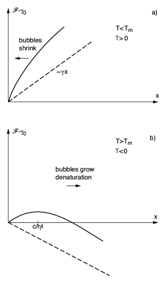
Figure 1: We depict the free energy profile $\mathscr{F}-\gamma_{0}$ below and above the melting temperature $T_{m}$ as a function of bubble size. In a) we show $\mathscr{F}-\gamma_{0}$ for $\gamma>0$, i.e., $T<T_{m}$; in b) we show $\mathscr{F}-\gamma_{0}$ for $\gamma<0$, i.e., $T>T_{m}$. For large bubble sizes, $x\gg x_{1}$ the free energy behaves approximately linearly as function of bubble size. For small bubble sizes the free energy has a logarithmic sink corresponding to the absorbing state at $x=0$ (arbitrary units). Above melting, there exists a nucleation barrier that needs to be crossed before the bubble is allowed to grow towards full denaturation. In both cases, the comparatively high initiation barrier $\gamma_{0}$ has to be overcome to seed the bubble.

The stochastic bubble dynamics in the free energy landscape $\mathscr{F}$ is described by the Langevin equation

$$\frac{dx}{dt}=-D\frac{d\mathscr{F}}{dx}+\xi,$$ (5)

driven by thermal noise $\xi$, that is characterized by the correlation function

$$\langle\xi(t)\xi(t^{\prime})\rangle=2DkT\delta(t-t^{\prime}).$$ (6)

The kinetic coefficient $D$ of dimension $(kT)^{-1}s^{-1}$ sets the inverse time scale of the dynamics. Inserting the free energy (2) in Eq. (5) we have in particular

$$\frac{dx}{dt}=\Omega_{2}-\frac{\Omega_{1}}{x}+\xi,$$ (7)

where we have found it convenient to introduce the inverse time scales $\Omega_{1}$ and $\Omega_{2}$,

$$\Omega_{1}=DckT,$$ (8a)

$$\Omega_{2}=-D\gamma=D\gamma_{1}(T-T_{m})/T_{m}.$$ (8b)

Note that the characteristic bubble size $x_{1}=ckT/|\gamma|$ is given by

$$x_{1}=\frac{ckT}{\gamma}=\frac{\Omega_{1}}{|\Omega_{2}|}$$ (9)

and thus emerges from the time scale competition between the $\Omega_{i}$, from a dynamic point of view.

In the limits of large and small bubble sizes, the Langevin equation (5) allows exact solutions:

(i) For large bubble size $x\gg x_{1}$ we can ignore the loop closure or entropic contribution $ckT/x$ and we obtain the Langevin equation

$$\frac{dx}{dt}=\Omega_{2}+\xi,$$ (10)

describing a 1D random walk with an overall drift velocity $\Omega_{2}$. For large $x$ we thus obtain the distribution Risken (1989)

$$P(x,t)=\frac{1}{\sqrt{4\pi DkTt}}\exp\left[-\frac{(x-x_{0}-\Omega_{2}t)^{2}}{4DkTt}\right],\leavevmode\nobreak\ \leavevmode\nobreak\$$ (11)

where $x_{0}$ is the initial (large) bubble size. It follows that the mean bubble size scales linearly with time, $\langle x\rangle=x_{0}+\Omega_{2}t$. Below $T_{m}$ ($\Omega_{2}<0$) the bubble size shrinks towards bubble closure; above $T_{m}$ ($\Omega_{2}>0$) the bubble size grows, leading to denaturation. The mean square bubble size fluctuations $\langle(\Delta x)^{2}\rangle=2DkTt$, increase linearly in time, a typical characteristic of a random walk.

Taking into account the absorbing state condition $P(x=0,t)=0$ for zero bubble size by forming the linear combination (method of images), we obtain for the distribution Redner (2001)

$$P_{\text{abs}}=\frac{1}{\sqrt{4\pi DkTt}}\left(\exp\left\{-\frac{(x-x_{0}-\Omega_{2}t)^{2}}{4DkTt}\right\}\right.$$

$$\left.-\exp\left\{-\frac{x_{0}\Omega_{2}}{DkT}\right\}\exp\left\{-\frac{(x+x_{0}-\Omega_{2}t)^{2}}{4DkTt}\right\}\right),\hskip 11.38092pt$$ (12)

and infer, using the definition Redner (2001)

$$W(t)=-\int_{0}^{\infty}dx\frac{\partial P_{\text{abs}}}{\partial t},$$ (13)

the first passage time density

$$W(t)=\frac{x_{0}}{\sqrt{4\pi DkTt^{3}}}\exp\left(-\frac{(x_{0}+\Omega_{2}t)^{2}}{4DkTt}\right).$$ (14)

with the typical Sparre Andersen asymptotics

$$W(t)\sim\frac{x_{0}}{\sqrt{4\pi DkT}}t^{-3/2}.$$ (15)

(ii) For small bubble size $x\ll x_{1}$ the nonlinear entropic term dominates and the bubble dynamics is governed by the nonlinear Langevin equation

$$\frac{dx}{dt}=-\frac{\Omega_{1}}{x}+\xi.$$ (16)

For vanishing noise Eq. (16) has the solution $x=(2\Omega_{1})^{1/2}(t_{0}-t)^{1/2}$ with $t_{0}=x_{0}/2\Omega_{1}$ in terms of the initial bubble size $x_{0}$ and thus exhibits a finite time singularity for $x=0$, i.e., a zero bubble size or bubble closure at time $t_{0}$. In Fig. 2 we have depicted the finite-time-singularity solution for vanishing noise together with the noisy case.

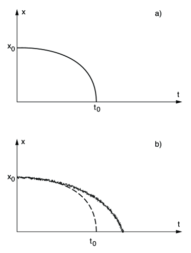
Figure 2: In a) we show the time evolution of a small bubble of size $x$ in the absence of thermal noise. For $x=0$ corresponding to bubble closure we encounter a finite-time-singularity at $t_{0}=x_{0}/2\Omega_{1}$. In b) we depict the noisy case. Here the first passage time is a statistical event characterized by $W(t)$ (arbitrary units).

In the presence of thermal noise Eq. (16) admits an exact solution, see e.g. Ref. Fogedby and Poutkaradze (2002). The probability distribution, subject to the absorbing state condition $P(0,t)=0$, has the form

$$P(x,t) = \frac{x^{\Omega_{1}/2DkT+1/2}}{x_{0}^{\Omega_{1}/DkT-1/2}}\frac{e^{-(x^{2}+x_{0}^{2})/4DkTt}}{2DkTt}$$ (17)

$$\times I_{1/2+\Omega_{1}/2DkT}\left(\frac{xx_{0}}{2DkTt}\right).$$

Here $I_{\nu}$ is the Bessel function of imaginary argument, $I_{\nu}(z)=(-i)^{\nu}J_{\nu}(iz)$ Lebedev (1972). Correspondingly, we find the first passage time distribution

$$W(t)= \frac{4DkTx_{0}^{1+\Omega_{1}/DkT}}{\Gamma(1/2-\Omega_{1}/2DkT)}\exp\left(-\frac{x_{0}^{2}}{4DkTt}\right)$$ (18)

$$\times(4DkTt)^{-3/2-\Omega_{1}/2DkT}$$

with the long time tail

$$W(t)\sim\frac{x_{0}^{1+\Omega_{1}/DkT}t^{-3/2-c/2}}{\Gamma(1/2-\Omega_{1}/2DkT)(4DkT)^{1/2+\Omega_{1}/2DkT}},$$ (19)

where we substituted back for $\Omega_{1}$: For small bubble sizes, the exponent $c$ due to the polymeric interactions changes the first passage statistics. As already noted in Ref. Fogedby and Metzler (2007), this modified exponent for $c>1$ gives rise to a finite mean first passage time $\int_{0}^{\infty}tW(t)dt$, in contrast to the first passage time distribution (14)

In the general case for bubbles of all sizes the fluctuations of double-stranded DNA is described by Eq. (7). The associated Fokker-Planck equation for the distribution $P(x,t)$ has the form (compare also Refs. Hanke and Metzler (2003); Bar et al. (2007); Fogedby and Metzler (2007))

$$\frac{\partial P}{\partial t}=\frac{\partial}{\partial x}\left(-\Omega_{2}+\frac{\Omega_{1}}{x}\right)P+DkT\frac{\partial^{2}P}{\partial x^{2}},$$ (20)

and provides the complete description of the single bubble dynamics in double-stranded homopolymer DNA in the continuum limit of the Poland-Scheraga model. For large bubble sizes where the entropic term $\Omega_{1}/x$ can be neglected the solution of Eq. (20) is given by Eqs. (11) and (12). Conversely, for small bubble sizes, where the entropic term $\Omega_{1}/x$ dominates, or for all bubble sizes precisely at the transition temperature $\Omega_{2}=0$ ($T=T_{m}$), the solution of Eq. (20) is given by the noisy finite-time-singularity solution in Eqs. (17) and (18).

III Weak noise analysis

In the weak noise limit $DkT\rightarrow 0$ we can apply a well-established canonical scheme to investigate the Fokker-Planck equation (20), see, for instance, Refs. Fogedby (1999, 2003). Introducing the WKB ansatz

$$P(x,t)\propto\exp\left(-\frac{S(x,t)}{2DkT}\right),$$ (21)

the weight (or action) $S(x,t)$ satisfies the Hamilton-Jacobi equation

$$\frac{\partial S}{\partial t}+H=0$$ (22)

with Hamiltonian

$$H=\frac{1}{2}p^{2}-p\left(-\Omega_{2}+\frac{\Omega_{1}}{x}\right).$$ (23)

From this scheme, the equations of motion yield in the form

$$\frac{dx}{dt}=\left(\Omega_{2}-\frac{\Omega_{1}}{x}\right)+p,$$ (24)

$$\frac{dp}{dt}=-\frac{\Omega_{1}}{x^{2}}p.$$ (25)

They determine orbits in a canonical phase space spanned by the bubble size $x$ and the momentum $p$. Comparing the equation of motion (24) with the Langevin equation (7) we observe that the thermal noise $\xi$ is replaced by the momentum $p=\partial S/\partial x$.

The action $S$ associated with an orbit from $x_{0}$ to $x$ during time $t$ is given by

$$S(x,t)=\int_{x_{0},0}^{x,t}dt\leavevmode\nobreak\ p\frac{dx}{dt}-Ht,$$ (26)

or by insertion of Eq. (24)

$$S(x,t)=\frac{1}{2}\int_{x_{0},0}^{x,t}dt\leavevmode\nobreak\ p^{2}.$$ (27)

III.1 Large bubbles

For large bubbles, i.e., $x\gg x_{1}=\Omega_{1}/|\Omega_{2}|$, we can ignore the loop closure contribution characterized by $\Omega_{1}$, and we obtain the Hamiltonian

$$H=\frac{1}{2}p^{2}+\Omega_{2}p,$$ (28)

as well as the linear equations of motion

$$\frac{dx}{dt}=\Omega_{2}+p,$$ (29)

$$\frac{dp}{dt}=0.$$ (30)

The solution is given by $p=p_{0}$, $x=x_{0}+(p_{0}+\Omega_{2})t$ describing an orbit from $(x_{0},p_{0})$ to $(x,p_{0})$ in time $t$. Isolating $p_{0}=(x-x_{0}-\Omega_{2})/t$ and inserting in Eq. (27) we obtain the action

$$S(x,t)=\frac{1}{2}\frac{(x-x_{0}-\Omega_{2}t)^{2}}{t},$$ (31)

and inserted in Eq. (21) the biased random walk distribution (11). In Fig. 3 we have depicted the phase space for $\Omega_{1}=0$, i.e., in the large bubble-random walk case. The orbits are confined to the constant energy surfaces. We note in particular that the infinite time orbit lies on the $p=-\Omega_{2}$ manifold. We note, moreover, that in the large bubble case the weak noise case fortuitously yields the exact result for the distribution $P$.

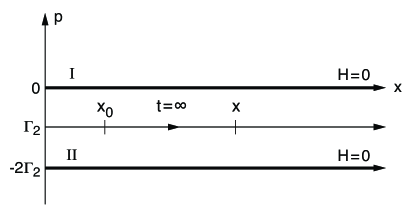
Figure 3: We show the phase space structure in the case $\Omega_{1}=0$, i.e., for random walk with constant drift. We show the zero energy manifolds for $p=0$ and $p=-2\Omega_{2}$ and a negative energy orbit from $x_{0}$ to $x$ in time $t$ (arbitrary units).

III.2 Small bubbles at and below $T_{m}$

For small bubbles, i.e., $x\ll x_{1}=\Omega_{1}/|\Omega_{2}|$, the loop closure contribution dominates and we obtain the Hamiltonian

$$H=\frac{1}{2}p^{2}-\frac{p\Omega_{1}}{x},$$ (32)

and the equations of motion

$$\frac{dx}{dt}=-\frac{\Omega_{1}}{x}+p,$$ (33)

$$\frac{dp}{dt}=-\frac{\Omega_{1}}{x^{2}}p,$$ (34)

determining orbits in $(x,p)$ phase space. Eliminating $p$ the bubble size is governed by the second order equation

$$\frac{d^{2}x}{dt^{2}}=-\frac{dV}{dx},$$ (35)

$$V=-\frac{\Omega_{1}^{2}}{2x^{2}},$$ (36)

describing the ’fall to the center’ ($x=0$) of a bubble of size $x$, i.e., the absorbing state corresponding to bubble closure.

The long time stochastic dynamics is here governed by the structure of the zero energy manifolds and fixed points. From Eq. (32) it follows that the zero energy manifold has two branches: i) $p=0$, corresponding to the noiseless transient behavior showing a finite time singularity as depicted in Fig. 2 and ii) $p=2\Omega_{1}/x$ associated with the noisy behavior. In Fig. 4 we have depicted the phase space structure.

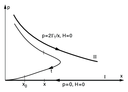
Figure 4: We show the phase space structure in the case $\Omega_{2}=0$ ($T=T_{m}$), i.e., for the small bubble dynamics governed by the entropic contribution. We show the zero energy manifolds $p=0$ and $p=2\Omega_{1}/x$ and a negative energy orbit from $x_{0}$ to $x$ in time $t$ (arbitrary units).

In the long time limit the orbit from $x_{0}$ to $x$ passes close to the zero energy manifold $p=2\Omega_{1}/x$. Inserted in the equation of motion (33) we have

$$\frac{dx}{dt}=\frac{\Omega_{1}}{x},$$ (37)

with long time solution

$$x(t)\sim(2\Omega_{1}t)^{1/2}.$$ (38)

We notice that the motion on the noisy manifold $p=2\Omega_{1}/x$ is time reversed of the motion on the noiseless manifold $p=0$. Next inserting the zero energy manifold condition $p=2\Omega_{1}/x$ in Eq. (27) we obtain

$$S=2\Omega_{1}^{2}\int dt\left(\frac{1}{x}\right)^{2},$$ (39)

and inserting the solution in Eq. (38) the action

$$S(x,t)=2\Omega_{1}\log x(t),$$ (40)

yielding according to Eq. (21) the long time distribution

$$P(x,t)\propto x(\Omega_{1}t)^{-\Omega_{1}/2DkT}.$$ (41)

We have incorporated the absorbing state condition $P=0$ for $x=0$; as discussed in Ref. Fogedby and Poutkaradze (2002) this condition follows from carrying the WKB weak noise approximation to next asymptotic order. For the first-passage time density of loop closure we obtain correspondingly

$$W(t)\propto t^{-\Omega_{1}/2DkT}.$$ (42)

We note that the power law dependence in Eqs. (41) and (42) is in accordance with Eqs. (17) and (18) for $DkT\rightarrow 0$.

IV Case of arbitrary noise strength

In the previous section we inferred weak noise-long time expressions for the distribution $P$ on the basis of a canonical phase space approach. Here we address the Fokker-Planck equation (20) in the general case. For the purpose of our discussion it is useful to introduce the parameters

$$\mu=c/2,$$ (43a)

$$\epsilon=\frac{\gamma_{1}}{2k}\left(\frac{1}{T_{m}}-\frac{1}{T}\right).$$ (43b)

Measuring time in units of $\mu\text{s}$ the Fokker-Planck equation (20) takes on the reduced form

$$\frac{\partial P}{\partial t}=\frac{\partial}{\partial x}\left(\frac{\mu}{x}-\epsilon\right)P+\frac{1}{2}\frac{\partial^{2}P}{\partial x^{2}}.$$ (44)

Note that $\mu\approx 1$, and, close to the physiological temperature $T_{\text{r}}$, $\epsilon\approx 2(T/T_{m}-1)$.

IV.1 Connection to the quantum Coulomb problem

By means of the substitution $P=e^{\epsilon x}x^{-\mu}\tilde{P}$, $\tilde{P}$ satisfies the equation Fogedby and Metzler (2007)

$$-\frac{\partial\tilde{P}}{\partial t}=-\frac{1}{2}\frac{\partial^{2}\tilde{P}}{\partial x^{2}}+\left(\frac{\mu(\mu+1)}{2x^{2}}-\frac{\mu\epsilon}{x}+\frac{\epsilon^{2}}{2}\right)\tilde{P},$$ (45)

which can be identified as an imaginary time Schrödinger equation for a particle with unit mass in the potential

$$V(x)=\frac{\mu(\mu+1)}{2x^{2}}-\frac{\mu\epsilon}{x}+\frac{\epsilon^{2}}{2},$$ (46)

i.e., subject to the centrifugal barrier $\mu(\mu+1)/x^{2}$ for an orbital state with angular momentum $\mu$ and a Coulomb potential $-\mu\epsilon/x$. In Fig. 5 we have depicted the potential $V-\epsilon^{2}/2$ in the two cases.

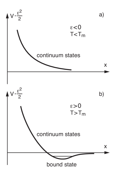
Figure 5: Schematic of the potential $V(x)-\epsilon^{2}/2$. a) $T<T_{m}$: The potential is repulsive, yielding a continuous spectrum. The bubble fluctuations correspond to a biased Brownian walk process in bubble size $x$ before collapse at $x=0$. b) $T<T_{m}$. The potential is attractive and can trap a series of bound states. At long times the lowest bound state indicated in the figure controls the behavior. The bubbles increase in size eventually leading to complete denaturation.

In terms of the Hamiltonian

$$H=-\frac{1}{2}\frac{d^{2}}{dx^{2}}+\frac{\mu(\mu+1)}{2x^{2}}-\frac{\mu\epsilon}{x}+\frac{\epsilon^{2}}{2},$$ (47)

the eigenvalue associated with Eq. (45) problem has the form

$$H\Psi_{n}=E_{n}\Psi_{n}.$$ (48)

Expressed in terms of the eigenfunctions the transition probability $P(x,x_{0},t)$ then becomes

$$P(x,x_{0},t)=e^{\epsilon(x-x_{0})}\left(\frac{x_{0}}{x}\right)^{\mu}\sum_{n}e^{-E_{n}t}\Psi_{n}(x)\Psi_{n}(x_{0}).$$

(49)

Here, the completeness of $\Psi_{n}$ ensures the initial condition $P(x,x_{0},0)=\delta(x-x_{0})$. Moreover, in order to account for the absorbing boundary condition for vanishing bubble size we choose $\Psi_{n}(0)=0$. We also note that for a finite strand of length $L$, i.e., a maximum bubble size of $L$, we have in addition the absorbing condition $\Psi_{n}(L)=0$ for complete denaturation. Expression (49) is the basis for our discussion of DNA-breathing, relating the dynamics to the spectrum of eigenstates, i.e., the bound and scattering states of the corresponding Coulomb problem Landau and Lifshitz (1959).

The transition probability $P(x,x_{0},t)$ for the occurrence of a DNA bubble of size $x$ at time $t$ is controlled by the Coulomb spectrum. Below the melting temperature $T_{m}$ for $\epsilon\propto(T/T_{m}-1)<0$, the Coulomb problem is repulsive and the states form a continuum, corresponding to a random walk in bubble size terminating in bubble closure $(x=0)$. At the melting temperature $T_{m}$ for $\epsilon=0$, the Coulomb potential is absent and the continuum of states is governed by the centrifugal barrier alone, including the limiting case of a regular random walk. Above the melting temperature for $\epsilon>0$, the Coulomb potential is attractive and can trap an infinity of bound states; at long times it follows from Eq. (49) that the lowest bound state in the spectrum dominates the bubble dynamics, corresponding to complete denaturation of the DNA chain.

Mathematically, we model the bubble dynamics with absorbing boundary conditions at zero bubble size $x=0$, and, for a finite chain of length $L$, at $x=L$. When the bubble vanishes or complete denaturation is reached, that is, the dynamics stops. Physically, this stems from the observation that on complete annihilation (closure) of the bubble, the large bubble initiation barrier prevents immediate reopening of the bubble. Similarly, a completely denatured DNA needs to re-establish bonds between bases, a comparatively slow diffusion-reaction process.

IV.1.1 Long times for $T<T_{m}$

At long times and fixed $x$ and $x_{0}$, it follows from Eq. (49) that the transition probability is controlled by the bottom of the energy spectrum. Below and at $T_{m}$ the spectrum is continuous with lower bound $\epsilon^{2}/2$. Setting $E_{k}=\epsilon^{2}/2+k^{2}/2$ in terms of the wavenumber $k$ and noting from the eigenvalue problem in Eqs. (47) and (48) that $\Psi_{k}(x)\sim(kx)^{1+\mu}$ for small $kx$ we find

$$P(x,x_{0},t) \propto \exp\left(-|\epsilon|(x-x_{0})\right)\left(\frac{x_{0}}{x}\right)^{\mu}\exp\left(-\frac{\epsilon^{2}t}{2}\right)$$

$$\times\int_{0}^{\infty}dke^{-k^{2}t/2}(k^{2}xx_{0})^{1+\mu}.$$

By a simple scaling argument we then obtain the long time expression for the probability distribution

$$P(x,x_{0},t)\propto xx_{0}^{1+2\mu}e^{-|\epsilon|(x-x_{0})}e^{-\epsilon^{2}t/2}t^{-3/2-\mu}.$$ (51)

The lifetime of a bubble of initial size $x_{0}$ created at time $t=0$ follows from Eq. (51) by calculating the first passing time density $W(t)$ in Eq. (13). Using the Fokker-Planck equation (44) we also have more conveniently

$$W(t)=\frac{1}{2}\left[\frac{\partial P}{\partial x}+\left(\frac{2\mu}{x}-2\epsilon\right)P\right]_{x=0},$$ (52)

and we obtain at long times

$$W(t)\propto(1+2\mu)x_{0}^{1+2\mu}e^{|\epsilon|x_{0}}e^{-\epsilon^{2}t/2}t^{-3/2-\mu}.$$ (53)

In Fig. 6 we have depicted the bubble lifetime distribution $W(t)$ below $T_{m}$ for $\epsilon=-1/2$.

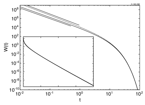
Figure 6: Bubble lifetime distribution $W(t)$ from Eq. (53), with $\epsilon=-1/2$, $x_{0}=5$, and $c=1.76$ (full line) and $2.12$ (dashed). The initial power-law behavior with slopes -2.38 and -2.56 is indicated by the straight lines. Inset: $\log$ versus linear scale, emphasizing the exponential decay for long times.

IV.1.2 At the transition $T=T_{m}$ ($\epsilon=0$)

At the transition temperature $T=T_{m}$ for $\epsilon=0$ the Coulomb term is absent and we have a free particle subject to the centrifugal barrier $\mu(\mu+1)/2x^{2}$. In this case the eigenfunctions are given by the Bessel function Lebedev (1972)

$$\Psi_{k}(x)=(kx)^{1/2}J_{1/2+\mu}(kx),$$ (54a)

$$E_{k}=\frac{k^{2}}{2},$$ (54b)

where orthogonality and completeness follow from the Fourier-Bessel integral Lebedev (1972)

$$f(x)=\int_{0}^{\infty}kJ_{\nu}(kx)dk\int_{0}^{\infty}yJ_{\nu}(ky)f(y)dy$$ (55)

By insertion into Eq. (49) we obtain the distribution

$$P(x,x_{0},t) = \frac{x_{0}^{1/2+\mu}}{x^{\mu-1/2}}$$

$$\times\int_{0}^{\infty}dke^{-k^{2}t/2}kJ_{1/2+\mu}(kx)J_{1/2+\mu}(kx_{0}),$$

or, by means of the identity Lebedev (1972)

$$\int_{0}^{\infty}e^{-tx^{2}}J_{p}(ax)J_{p}(bx)xdx=\frac{1}{2t}e^{-(a^{2}+b^{2})/4t}I_{p}\left(\frac{ab}{2t}\right),$$ (56)

the explicit expression

$$P(x,x_{0},t) = \left(\frac{x_{0}}{x}\right)^{\mu}(xx_{0})^{1/2}t^{-1}e^{-(x^{2}+x_{0}^{2})/2t}$$ (57)

$$\times I_{1/2+\mu}(xx_{0}/t).$$

Here, $I_{\nu}(z)$ is the Bessel function of imaginary argument Lebedev (1972). From Eq. (57) we also infer, using Eq. (52) the first passage time distribution

$$W(t)=\frac{2x_{0}^{1+2\mu}}{\Gamma(1/2+\mu)}e^{-x_{0}^{2}/2t}(2t)^{-3/2-\mu},$$ (58)

in accordance with Eq. (53) for $\epsilon=0$. In Fig. 7 we show the first passage time distribution (58) for two different critical exponents $c$. Note that the power-law exponent $-3/2-\mu=-3/2-c/2$ is identical to the result reported in Ref. Bar et al. (2007).

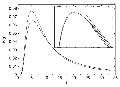
Figure 7: Bubble lifetime distribution $W(t)$ from Eq. (58) for $T=T_{m}$, $x_{0}=5$, as well as $c=1.76$ (full line) and $c=2.12$ (dashed line). Inset: $\log$-$\log$ plot of the power-law behavior at long $t$, with slopes $-2.38$ and $-2.56$, as indicated by the straight lines.

IV.1.3 Long times for $T>T_{m}$

Above the transition temperature for $\epsilon>0$ the Coulomb potential $-\mu\epsilon/x$ is attractive and can trap a series of bound states. In the long time limit the lowest bound state controls the behavior of $P$. According to Eqs. (47) and (48) the lowest bound state $\Psi_{1}$ with eigenvalue $E_{1}<\epsilon^{2}/2$ must satisfy the eigenvalue equation

$$\left[-\frac{1}{2}\frac{d^{2}\Psi_{1}}{dx^{2}}+\frac{\mu(\mu+1)}{2x^{2}}-\frac{\mu\epsilon}{x}+\frac{\epsilon^{2}}{2}\right]\Psi_{1}=E_{1}\Psi_{1}.$$ (59)

For $x\rightarrow\infty$ we have $-(1/2)\Psi_{1}^{\prime\prime}=(E_{1}-\epsilon^{2}/2)\Psi_{1}$ and $\Psi_{1}$ must fall off exponentially, $\Psi_{1}\sim\exp(-\lambda x)$, $\lambda=(2E_{1}-\epsilon^{2})^{1/2}$. For $x\rightarrow 0$ we have $-(1/2)\Psi_{1}^{\prime\prime}+(\mu(\mu+1)/2x^{2})\Psi_{1}\sim 0$ and we infer $\Psi_{1}\sim x^{1+\mu}$. Consequently, searching for a nodeless bound state of the form $\Psi_{1}\sim x^{1+\mu}\exp(-\lambda x)$ we readily obtain the normalized lowest level

$$\Psi_{1}(x)=Ax^{1+\mu}e^{-\mu\epsilon x/(1+\mu)},$$ (60a)

$$A^{2}=\frac{(2\mu\epsilon/(\mu+1))^{2\mu+3}}{\Gamma(2\mu+3)},$$ (60b)

with corresponding eigenvalue

$$E_{1}=\frac{\epsilon^{2}}{2}\left(1-\left(\mu/(\mu+1)\right)^{2}\right).$$ (61)

The maximum of the bound state is located at $(\mu+1)^{2}/\mu\epsilon\sim 1/(T-T_{m})$ and thus recedes to infinity as we approach the melting temperature. From Eq. (49) we thus obtain after some reduction

$$P(x,x_{0},t) = A^{2}xx_{0}^{1+2\mu}e^{(\epsilon/(1+\mu))(x-x_{0}(1+2\mu))}$$ (62)

$$\times e^{-\epsilon^{2}(1+2\mu)t/2(1+\mu)^{2}}.$$

Above $T_{m}$ the bubble size, on average, increases in time until full denaturation is reached. In terms of the free energy plot in Fig. 1b this corresponds to a Kramers escape across the (soft) potential barrier (corresponding to a nucleation process). This implies that the transition probability $P(x,x_{0},t)$ from an initial bubble size $x_{0}$ to a final bubble size $x$ must vanish in the limit of large $t$. According to Eq. (62) $P(x,x_{0},t)$ decays exponentially,

$$P(x,x_{0},t)\propto e^{-t/\tau}$$ (63)

with a time constant given by

$$\tau=\frac{2(1+\mu)^{2}}{(1+2\mu)\epsilon^{2}}\propto|T-T_{m}|^{-2}$$ (64)

IV.2 Exact results

The eigenvalue problem given by Eqs. (47) and (48)

$$\left[-\frac{1}{2}\frac{d^{2}\Psi}{dx^{2}}+\frac{\mu(\mu+1)}{2x^{2}}-\frac{\mu\epsilon}{x}+\frac{\epsilon^{2}}{2}\right]\Psi=E\Psi,$$ (65)

has the same form as the differential equation satisfied by the Whittaker function $w$ Gradshteyn and Ryzhik (1965),

$$-\frac{d^{2}w}{dx^{2}}+\left(\frac{1}{4}-\frac{\lambda}{z}-\frac{1/4-m^{2}}{z^{2}}\right)w=0,$$ (66)

with the identifications $z=2\kappa x$, $\lambda=\mu\epsilon/\kappa$, $m=1/2+\mu$, and $E=\epsilon^{2}/2-\kappa^{2}/2$. Incorporating the absorbing state condition $\Psi(0)=0$ and using an integral representation for the Whittaker function $w$ Gradshteyn and Ryzhik (1965) we obtain the solution

$$\Psi(x) \propto (2\kappa x)^{1+\mu}e^{-\kappa x}$$

$$\times\int_{0}^{\infty}e^{-2\kappa xt}t^{\mu(1-\epsilon/\kappa)}(1+t)^{\mu(1+\epsilon/\kappa)}dt.$$

In the bound state case for $\epsilon>0$ the parameter $\kappa>0$ and the bound state spectrum is obtained by terminating the power series expansion of Eq. (LABEL:int)Gradshteyn and Ryzhik (1965),

$$\Psi(x) \propto (2\kappa x)^{1+\mu}e^{-\kappa x}$$ (68)

$$\times\Phi(1+\mu(1-\epsilon/\kappa),2(1+\mu);2\kappa x),$$

with the polynomial

$$\Phi(\alpha,\gamma;z) = 1+\frac{\alpha}{\gamma}\frac{z}{1!}+\frac{\alpha(\alpha+1)}{\gamma(\gamma+1)}\frac{z^{2}}{2!}$$ (69)

$$+\frac{\alpha(\alpha+1)(\alpha+2)}{\gamma(\gamma+1)(\gamma+2)}\frac{z^{3}}{3!}.$$

Simple algebra then yields the spectrum

$$\kappa=\epsilon\frac{\mu}{\mu+n},\leavevmode\nobreak\ \leavevmode\nobreak\ n=1,2,\cdots$$ (70)

and associated eigenfunctions

$$\Psi\propto x^{1+\mu}e^{-\kappa x}\times\text{polynomial},$$ (71)

the lowest state and eigenfunctions given by Eqs. (60a) and (61).

V Discussion

In typical experiments measuring fluorescence correlations of a tagged base pair bubble breathing can be measured on the level of a single DNA molecule Bonnet et al. (1998); Altan-Bonnet et al. (2003). The correlation function $C(t)$ is proportional to the integrated survival probability, i.e.,

$$C(t)\propto\int_{0}^{L}P(x,x_{0},t)dx,$$ (72)

where $L$ is the chain length. From the definition of the first passage time distribution in Eq. (13) we also have

$$C(t)=1-\int_{0}^{t}W(t^{\prime})dt^{\prime}.$$ (73)

V.1 Below $T_{m}$ for $\epsilon<0$

Below the melting temperature $T_{m}<0$ we obtain from Eq. (53)

$$C(t)=1-x_{0}^{1+2\mu}e^{|\epsilon|x_{0}}\int_{0}^{t}e^{-\epsilon^{2}t^{\prime}/2}(t^{\prime})^{-3/2-\mu}dt^{\prime},$$ (74)

or in terms of the incomplete Gamma function $\gamma(\alpha,x)=\int_{0}^{x}e^{-t}t^{\alpha-1}dt$ Lebedev (1972)

$$C(t) = 1-x_{0}^{1+2\mu}e^{|\epsilon|x_{0}}(\epsilon^{2}/2)^{1/2+\mu}$$ (75)

$$\times\gamma(-1/2-\mu,\epsilon^{2}t/2).$$

Using $\gamma(\alpha,x)=\Gamma(\alpha)-x^{\alpha-1}e^{-x}$ for $x\rightarrow\infty$ we have for large $t$

$$C(t)=\text{const.}+x_{0}^{1+2\mu}\epsilon^{-2}e^{|\epsilon|x_{0}}t^{-3/2-\mu}e^{-\epsilon^{2}t/2}.$$ (76)

We note that the basic time scale of the correlations is set by $\epsilon^{-2}\propto(T_{m}-T)^{-2}$. As we approach $T_{m}$ the time scale diverges like $(T_{m}-T)^{-2}$.

For $t\ll\epsilon^{-2}$ the correlations show a power law behavior

$$C(t)=\text{const.}+C(t)\propto t^{-3/2-\mu}\text{(mod a const.)},$$ (77)

with scaling exponent $-3/2-\mu=-3/2-c/2$. Here $3/2$ originates from unbiased bubble size random walk whereas the contribution $\mu=c/2$ is associated with the entropy loss of a closed polymer loop.

At long times $t\gg\epsilon^{-2}$ the correlations fall off exponentially

$$C(t)=\text{const.}+C(t)\propto e^{-\epsilon^{2}t/2}\text{(mod a const.)}.$$ (78)

The size of the time window showing power law behavior increases as $T_{m}$ is approached. This corresponds to the critical slowing down on denaturation, as already observed in Ref. Ambjörnsson et al. (2006) numerically, and in Ref. Bicout and Kats (2004) in absence of the critical exponent $c$ due to polymeric interactions.

In frequency space the structure function is given by

$$\tilde{C}(\omega)=\int e^{i\omega t}C(t)dt.$$ (79)

By means of a simple scaling argument we infer that $\tilde{C}(\omega)$ has a Lorentzian line shape for $|\omega|\ll\epsilon^{2}$ crossing over to power law tails for $|\omega|\gg\epsilon^{2}$.

$$\tilde{C}(\omega)\sim x_{0}^{1+2\mu}e^{|\epsilon|x_{0}}\frac{1}{\omega^{2}+(\epsilon^{2}/2)^{2}}\leavevmode\nobreak\ \leavevmode\nobreak\ \text{for}\leavevmode\nobreak\ \leavevmode\nobreak\ |\omega|\ll\epsilon^{2}\leavevmode\nobreak\ \leavevmode\nobreak\ \leavevmode\nobreak\ \leavevmode\nobreak\ \leavevmode\nobreak\ \leavevmode\nobreak\$$ (80a)

$$\tilde{C}(\omega)\sim x_{0}^{1+2\mu}e^{|\epsilon|x_{0}}\frac{1}{\epsilon^{2}}|\omega|^{1/2+\mu}\leavevmode\nobreak\ \leavevmode\nobreak\ \leavevmode\nobreak\ \leavevmode\nobreak\ \leavevmode\nobreak\ \text{for}\leavevmode\nobreak\ \leavevmode\nobreak\ |\omega|\gg\epsilon^{2}$$ (80b)

In Fig. 8 we have depicted the structure function $\tilde{C}(\omega)$.

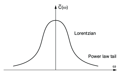
Figure 8: The structure function $\tilde{C}(\omega)$. For $|\omega|\ll\epsilon^{2}$ the structure function has a Lorentzian line shape; for $|\omega|\gg\epsilon^{2}$ it exhibits power law tails.

V.2 At $T_{m}$ for $\epsilon=0$

At the transition temperature $T_{m}$ the exact expression for the first passage time distribution is given by Eq. (58). Using Eq. (73) for $C(t)$ we then obtain

$$C(t)=1-\frac{\Gamma(1/2+\mu,x_{0}^{2}/2t)}{\Gamma(1/2+\mu)},$$ (81)

where $\Gamma(\alpha,x)=\int_{x}^{\infty}e^{-t}t^{\alpha-1}dt$ is the incomplete Gamma function Lebedev (1972).

At short times we have

$$C(t)=1-\frac{(x_{0}^{2}/2)^{\mu-1/2}}{\Gamma(1/2+\mu)}t^{1/2-\mu}e^{-x_{0}^{2}/2t},$$ (82)

whereas for $t\rightarrow\infty$

$$C(t)=\frac{2(x_{0}^{2})^{1/2+\mu}}{(1+2\mu)\Gamma(1/2+\mu)}t^{-1/2-\mu}.$$ (83)

The correlation function thus exhibits a power law behavior with scaling exponent $-1/2-\mu=-1/2-c/2$, as obtained from a different argument in Ref. Bar et al. (2007). Correspondingly, the structure function $\tilde{C}(\omega)$ has the form

$$\tilde{C}(\omega)\propto x_{0}^{1+2\mu}|\omega|^{\mu-1/2}.$$ (84)

V.3 Above $T_{m}$ for $\epsilon>0$

Above $T_{m}$ ($\epsilon>0$) the DNA chain eventually fully denatures and the correlations diverge in the thermodynamic limit. We can, however, at long times estimate the size dependence for a chain of length $L$. From the general expression (49) we find

$$C(t)\simeq e^{-\epsilon x_{0}}x_{0}^{\mu}\sum_{n}e^{-E_{n}t}\Psi_{n}(x_{0})\int_{0}^{L}e^{\epsilon x}x^{-\mu}\Psi_{n}(x)dx.$$

(85)

At long times the lowest bound state dominates the expression. Inserting $\Psi_{1}$ and $E_{1}$ from Eqs. (60a), (60b), and (61) and performing the integration over $x$ we obtain

$$C(t)\propto A^{2}e^{-\epsilon x_{0}(2\mu+1)/(\mu+1)}e^{-\epsilon^{2}((\mu+1/2)/(\mu+1)^{2})t}x_{0}^{1+2\mu}$$

$$\times(1+\mu)\epsilon^{-2}\left[1+(L\epsilon/(1+\mu)-1)e^{\epsilon L/(1+\mu)}]\right].$$ (86)

The correlations decay exponentially with time constant $\sim\epsilon^{-2}(\mu+1)^{2}/(2\mu+1)$. In frequency space the structure function has a Lorentzian lineshape of width $\sim\epsilon^{2}(2\mu+1)/(\mu+1)^{2}$, and for the size dependence one obtains

$$C(t)\sim\left\{\begin{array}[]{ll}Le^{\epsilon L/(1+\mu)},&\mbox{for }\epsilon L/(1+\mu)\gg 1,\\[5.69046pt] L\epsilon/(1+\mu),&\mbox{for }\epsilon L/(1+\mu)\ll 1\end{array}\right..$$ (87)

Note that close to $T_{m}$ the correlation function $C(t)\propto L$. In Fig. 9 we depict in a plot of $C/L$ vs. $L$ the size dependence of the correlation function.

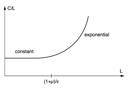
Figure 9: We depict $C/L$ as a function of $L$. For $L\ll(1+\mu)/\epsilon$ the correlations depends linearly on $L$; for $L\gg(1+\mu)/\epsilon$ the correlations increase exponentially as a function of $L$.

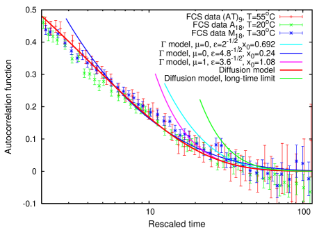
Figure 10: (Color online). Drift-diffusion model and experimental data from Ref.Altan-Bonnet et al. (2003) compared to the $\Gamma$ model, for various parameters. The curve for $\mu=0$ and $\epsilon=1/\sqrt{2}$ exactly matches the long-time behavior from Ref. Altan-Bonnet et al. (2003).

V.4 Comparison to experimental data

Below the melting temperature $T_{m}$, DNA breathing can be monitored on the single DNA level by fluorescence correlation spectroscopy Ambjörnsson et al. (2006); Ambjörnsson et al. (2007a); Altan-Bonnet et al. (2003). In the FCS experiment from Ref. Altan-Bonnet et al. (2003), a DNA construct of the form

$$\begin{array}[]{l}\mbox{{{\color[rgb]{1,1,1}5'GGCGCCCATATATATATA}F{\color[rgb]{1,1,1}ATATATATGCGCTT}}}\\[-1.42271pt] \mbox{{5'{\color[rgb]{1,1,1}GGCGCCCATATATATATA}|{\color[rgb]{1,1,1}ATATATATGCGC}T{\color[rgb]{1,1,1}T}}}\\[-1.42271pt] \mbox{{{\color[rgb]{1,1,1}5'}GGCGCCCATATATATATATATATATATGCGC{\color[rgb]{1,1,1}T}T}}\\[-1.42271pt] \mbox{{{\color[rgb]{1,1,1}3'}CCGCGGGTATATATATATATATATATACGCG{\color[rgb]{1,1,1}T}T}}\\[-1.42271pt] \mbox{{3'{\color[rgb]{1,1,1}GGCGCCCATATATATAT}|{\color[rgb]{1,1,1}TATATATATGCGC}T{\color[rgb]{1,1,1}T}}}\\[-1.42271pt] \mbox{{{\color[rgb]{1,1,1}5'GGCGCCCATATATATAT}Q{\color[rgb]{1,1,1}TATATATATGCGCTT}}}\end{array}$$ (88)

was employed. Here, a bubble domain consisting of weaker AT base pairs are clamped by stronger GC base pairs. On the right, a short loop consisting of four T nucleotides is introduced. The fluorophore (F) and quencher (Q) are attached to T nucleotides as shown. With the highest probability, a bubble will form in the AT-bubble domain. As the bubbles consist of flexible single-strand, in an open bubble the fluorophore and quencher move away from each other, and fluorescence occurs. Once in the focal volume of the FCS setup, bubble opening and closing corresponds to blinking events in the signal, whose correlation function (corrected for the diffusion in and out of the focal volume) are shown in Fig. 10. Three different bubble domains with changing sequence were used to check that potential secondary structure formation does not influence the breathing dynamics, confirming the picture of base pair-after-base pair zipping and unzipping. The figure shows examples from all three constructs, underlining the data collapse already observed in Ref. Altan-Bonnet et al. (2003).

The theoretical lines shown in Fig. 10 correspond to the biased diffusion model introduced in the original article Altan-Bonnet et al. (2003). While the full solution of this diffusion model fits the data well over the entire window, the long time expansion demonstrates the rather weak convergence of the expansion. In Fig. 10 we also included our asymptotic solution (75) for the autocorrelation function, for various parameters. Good agreement with the data is observed.

VI Summary and Conclusion

In this paper we have analyzed the breathing dynamics of thermally induced denaturation bubbles forming spontaneously in double-stranded DNA. We have shown that the Fokker-Planck equation can be analyzed from two points of view: i) In the weak noise or low temperature limit a canonical phase space approach interprets the stochastic dynamics in terms of a deterministic ’classical’ picture and gives by simple estimates access to the long time dynamics. In particular, we deduce that the dynamics at the transition temperature is characterized by power law behavior with scaling exponent depending on the entropic term. ii) In the general case we show that the Fokker-Planck equation can be mapped onto the imaginary time Schrödinger equation for a particle in a Coulomb potential. The low temperature region below the transition temperature then corresponds to the continuum states of a repulsive Coulomb potential, whereas the region above $T_{m}$ is controlled by the lowest bound state in an attractive Coulomb potential. The mapping, moreover, allows us to calculate the distribution of bubble lifetimes and the associated correlation functions, below, at, and above the melting temperature of the DNA helix-coil transition. Finally, at the melting transition, the DNA bubble-breathing was revealed to correspond to a one-dimensional finite time singularity.

The analysis reveals non-trivial scaling of the first passage time density quantifying the survival of a bubble after its original nucleation. The associated critical exponent depends on the parameter $\mu=c/2$ stemming from the entropy loss factor of the flexible bubble. The first passage time distribution and correlations depend on the difference $T/T_{m}-1$, and therefore explicitly on the melting temperature $T_{\mathrm{m}}$ (and thus the relative content of AT or GC base pairs). We also obtained the critical dependence of the characteristic time scales of bubble survival and correlations on the difference $T-T_{m}$. The finite size-dependence of the correlation function was recovered, as well.

The mapping of the of DNA-breathing onto the quantum Coulomb problem provides a new way to investigate its physical properties, in particular, in the range above the melting transition, $T>T_{m}$. The detailed study of the DNA bubble breathing problem is of particular interest as the bubble dynamics provides a test case for new approaches in small scale statistical mechanical systems where the fluctuations of DNA bubbles are accessible on the single molecule level in real time.