Thermal gradient-induced forces on geodetic reference masses for LISA

Abstract

The low frequency sensitivity of space-borne gravitational wave observatories will depend critically on the geodetic purity of the trajectories of orbiting test masses. Fluctuations in the temperature difference across the enclosure surrounding the free-falling test mass can produce noisy forces through several processes, including the radiometric effect, radiation pressure, and outgassing. We present here a detailed experimental investigation of thermal gradient-induced forces for the LISA gravitational wave mission and the LISA Pathfinder, employing high resolution torsion pendulum measurements of the torque on a LISA-like test mass suspended inside a prototype of the LISA gravitational reference sensor that will surround the test mass in orbit. The measurement campaign, accompanied by numerical simulations of the radiometric and radiation pressure effects, allows a more accurate and representative characterization of thermal-gradient forces in the specific geometry and environment relevant to LISA free-fall. The pressure dependence of the measured torques allows clear identification of the radiometric effect, in quantitative agreement with the model developed. In the limit of zero gas pressure, the measurements are most likely dominated by outgassing, but at a low level that does not threaten the LISA sensitivity goals.

I Introduction

LISA, the Laser Interferometer Space Antenna big , is a ESA-NASA mission to create the first spaceborne interferometric observatory of gravitational waves, in the frequency range between 30 $\mu$Hz and 1 Hz. LISA should permit not only detection, but detailed, high resolution, long measurement time observation of gravitational wave signals, opening the possibility for important discovery in fundamental physics, astrophysics, and cosmology.

LISA consists of three identical spacecraft separated by $5\times 10^{6}$ km, forming a nearly equilateral triangle that orbits the sun at a distance of 1 AU. Inside each spacecraft, there are two “free-falling” cubic test-masses (TM) in nominally geodesic motion. Gravitational waves are detected by an interferometric measurement of the relative change in the distances between distant free-falling TM caused by the gravitational wave metric perturbation. LISA aims at a gravitational wave strain noise floor of $4\times 10^{-21}\mathrm{/Hz^{1/2}}$ near 3 mHz, increasing as $1/f^{2}$ at lower frequencies. Performance at these lower frequencies is limited by the purity of the TM geodetic motion and requires perfect free-fall, along the sensitive interferometry axis (referred as the $x$ axis here), to within an acceleration noise of $3\times 10^{-15}\mathrm{m/s^{2}/Hz^{1/2}}$ ($3\>\mathrm{fm/s^{2}/Hz^{1/2}}$). For the 2 kg TM foreseen for LISA, this is equivalent to a force noise of 6 fN/Hz^1/2. While placing test particles in nearly perfect geodetic orbits inside of a controlled, co-orbiting spacecraft is essential to various space gravitational experiments, the extremely low force noise requirement and low measurement frequencies make LISA even more demanding in this respect than other previous (GPB GPB ) and future (STEP STEP , Microscope Microscope ) missions.

While the spacecraft shields the TM from environmental disturbances such as solar radiation pressure, it is itself a leading source of disturbing force acting on the TM. Achieving the required extremely low level of spurious acceleration requires identification and suppression of all interactions that can compete with gravity in defining the trajectory of the particle. The disturbances identified thus far have been collected in an overall noise model Dolesi et al. (2003); Stebbins et al. (2003); Schumaker et al. (2003)that has been used to optimize the LISA design.

Particular attention has been dedicated to the interaction between the TM and the position sensor that surrounds the TM and is used to guide precision thrusters that keep the spacecraft centered around the free-falling TMs. As such, the design of the TM and position sensor – referred to together as the “gravitational reference sensor” or GRS – is critical to achieving the LISA force noise goals. The current GRS is a 46 mm cubic TM of Au-Pt (2 kg) surrounded by an array of conducting electrode surfaces used for a capacitive position readout and force actuation scheme (see Fig.1 and Weber et al. (2002b); Dolesi et al. (2003)). The TM material is chosen for low magnetic susceptibility and residual moment, to minimize interaction with magnetic field noise Hueller et al. (2005). To reduce short range stray electrostatic effects, the distance (“gaps”) between the TM and the electrodes are relatively large, 4 mm on the interferometry axis, and all conducting surfaces are Au-coated to provide electrostatic homogeneity. To limit temperature differences across the TM, and thus also the temperature-gradient related forces which are the subject of this article, the sensor housing is made of a high thermal conductivity composite structure of molybdenum and sapphire.

The unprecedentedly small level of force noise needed for LISA requires measurement of the small disturbing forces in order to verify the feasibility of the gravitational wave sensitivity goals. Given the possibility of force noise sources that are not accurately modelled or perhaps not even previously identified, these tests should, as much as possible, use the final flight hardware configuration, reflecting not only the nominal design materials and geometry, but also the relevant machining, surface finishing, impurities, and cleanliness. Such testing is being pursued both in space, where the LISA Pathfinder mission will perform a dedicated flight test of the full LISA drag-free control system vitale:nuc:phys ; Anza et al. (2005), and on ground, where torsion pendulum dynamometers can characterize the force noise generated inside the GRS Hueller et al. (2002). A recent torsion pendulum study of the GRS capacitive sensor to be flown aboard LISA Pathfinder has demonstrated the absence of unknown surface forces to within roughly an order of magnitude of the LISA goal at 3 mHz Carbone et al. (2007). Other studies have measured important electrostatic and elastic coupling effectsCarbone et al. (2003, 2005); carbone:thesis ; Carbone et al. (2003); seattle . Ongoing work aims at extending these studies to lower force noise levels, lower frequencies, and to even more representative hardware configurations.

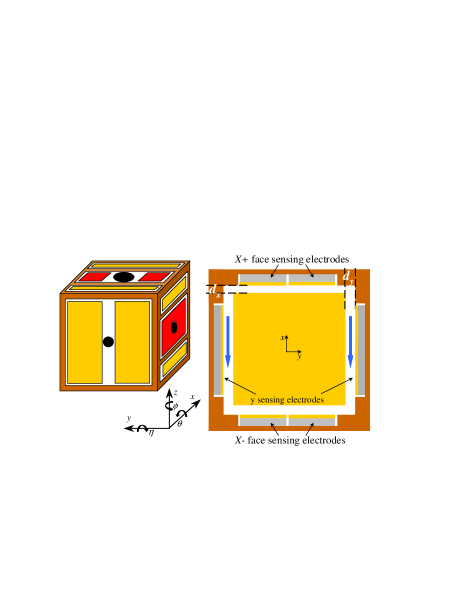
Figure 1: Schematic of the six degree of freedom capacitive position sensor for LISA Pathfinder and LISA. The sensor electrodes are obtained by Au-coating of an insulating substrate, mounted on an external metallic frame. At left, sensing electrodes are in orange, sensor bias injection electrode are red, and the supporting housing is brown. The black circles represent holes to allow access for laser light and for a TM caging mechanism during launch. The $x$ axis represents the sensitive LISA interferometry axis relevant for force noise. A internal section of the GRS is shown, with the blue arrows representing the path linking the two $X$ faces of the TM for gas and thermal photons. The TM-electrode gaps on the three axes are $d_{x}=4\>$ mm, $d_{y}=2.9\>$ mm and $d_{z}=3.5\>$ mm.

This paper describes a detailed study of the specific class of force noise induced by thermal gradients. Thermal gradient-induced forces have been modeled as part of the acceleration noise budget for LISA Schumaker et al. (2003); Stebbins et al. (2003); Dolesi et al. (2003); Nobili et al. (2001, 2002) and have been the subject of preliminary experimental investigations Carbone et al. (2005); carbone:thesis ; pollack:thermal . A temperature difference between the sensor surfaces on opposing sides of the TM converts into a net force through at least three mechanisms: the radiometric effect, differential radiation pressure, and temperature dependent outgassing. Broadly speaking, the radiometric and radiation pressure forces arise in the temperature dependence of the momentum transferred to a TM face by impacts of, respectively, residual gas molecules and thermal photons. If, at the LISA operating temperature (293 K) and pressure (10^-5 Pa), we apply a simplified “infinite plate” model - to be discussed, along with its limitations and a more accurate simulation, in Sec. II – the radiometric and radiation pressure effects can be estimated to produce $\frac{dF}{d\Delta T}$, a net force per degree of temperature difference, of roughly 20 and 30 pN/K, respectively, always pointing from the hot side of the sensor towards the cold. A third effect, more difficult to model and dependent on surface cleanliness, arises in the temperature dependence of outgassing from the sensor surfaces and the net momentum thus imparted on the TM by desorbed molecules in the presence of a thermal gradient. As will be discussed in the following section, this effect has been expected to contribute roughly as much as the other two effects. The three effects respond coherently to the same temperature gradient and sum to give a net temperature-difference response of roughly $\frac{dF}{d\Delta T}\approx$ 100 pN/K.

This estimated “transfer function” sets the tolerable level of temperature difference fluctuations. In order to hold the thermal gradient-induced force noise to roughly $10\%$ of the overall force noise budget, the fluctuations in temperature difference across the GRS must be less than 10^-5 K/Hz^1/2. This level of temperature difference stability, which motivated the use of high thermal conductivity materials in the sensor, looks feasible but is challenging at the lowest frequencies, where the passive thermal filtering of solar radiation intensity fluctuations becomes progressively less effectiveBender ; Merko .

The article aims at a characterization, through experiment and simulation, of the thermal gradient transfer function $\frac{dF}{d\Delta T}$ relevant to LISA free-fall. This study is important to free-fall for LISA and other precision force measurements for several reasons. First, while the rough estimates discussed above for the radiation pressure and radiometric effects are readily obtained from simple formulas, they are based on an infinite plate model, which is not particularly accurate for the geometry of the proposed GRS, where the dimensions of the TM are only roughly 10 times larger than the TM-sensor gaps. As will be seen from the results of the simulations presented in App. A and App. B, these corrections, based on the geometry and, in the case of radiation pressure, surface reflectivity properties of the sensor, have a quantitative impact on the estimates of these noise sources for LISA and on the measurements presented here.

An even more important motivation for an experimental investigation lies in the large uncertainties with which we can estimate the outgassing effect, which will depend not only on the sensor geometry, but also on the amount, geometrical distribution, chemical nature, and history of the surface contamination inside the sensor. The amount to which the purity of free-fall is threatened by outgassing can only be reliably estimated through measurement with representative sensor hardware. The same argument can be applied to any other possible unmodelled or unidentified thermal related disturbance.

It should be noted that knowing the impact of thermal gradients can have an impact on the overall LISA experiment design, particularly on the amount of thermal filtering needed, or even whether active temperature control is necessary. Additionally, the measurement of $\frac{dF}{d\Delta T}$ can be repeated in-flight during the LISA and LISA Pathfinder missions, a “calibration” that, combined with the appropriate thermometer readings, will allow a correlation analysis of the noise and even a subtraction of the disturbance from the gravitational wave time series.

The experimental investigation was performed by means of a torsion pendulum, with a thin fiber suspending a hollow LISA-like test mass on-axis with its center of mass, inside a GRS prototype. Two prototype sensors were tested, the current LISA and LISA Pathfinder design showed in Fig.1, with 4, 3.5, and 2.9 mm gaps, and an earlier prototype with smaller gaps, 2 mm on all axes (these are described in Sec. III.1). The geometry of the pendulum is sensitive only to torques rather than the net forces that are relevant to $\frac{dF}{d\Delta T}$ along the LISA interferometer $x$ axis. As such, the basic measurement technique, described in detail in Sec. III, will be to apply a “rotational temperature gradient” such as to excite a measurable torque that is proportional to the applied heat and, through modelling of the different effects, to the transfer function $\frac{dF}{d\Delta T}$. The measurements, of excited torque as a function of the temperature gradient pattern and presented in Sec. IV, are performed for various sensor average temperatures and for a range of pressures, which allows a separation of the radiometric and radiation pressure effects from their known functional dependencies.

The pendulum configuration and the measurement of a torque (rather than a force) signal necessarily complicates the experimental analysis, demanding an interpolation of the relevant sensor temperature distribution from a limited array of thermometers and comparison with the torques calculated from the radiometric and radiation pressure models. In addition to complicating the analysis, the torque measurement imposed by the pendulum configuration means that the measurement will be blind to potential outgassing effects that act directly on the center of the TM faces, as there will be no “effective armlength” to convert such forces into measurable torques. However, in spite of these analysis difficulties, discussed in Sec. III, and the limitations of the torque measurement, to be discussed along with the study results in Sec. V, relevant conclusions can be drawn concerning the role of all relevant contributions to the overall thermal gradient effect for LISA free-fall.

II Modeling of thermal gradient-induced forces in the LISA GRS

In this section we describe the three main physical processes that convert fluctuating temperature gradients into noisy forces on the LISA TM. For the radiometric and radiation pressure effects, we present both the simplified models mentioned in the introduction and the results from numerical simulations using realistic sensor dimensions and surface properties. A thorough explanation of the simulations is given in Appendixes A and B.

In the discussion that follows, we assume the average GRS temperature to be $T_{0}$, with $T(\mathbf{r})$ the temperature distribution on the internal surface of the position sensor, facing the TM at a position $\mathbf{r}$. Given the high thermal conductivity of the sensor materials and the small expected thermal loads, we consider small temperature differences $\delta T(\mathbf{r})\equiv\left(T(\mathbf{r})-T_{0}\right)\ll T_{0}$. Additionally, as the thermal conductance across the TM is much greater than that between TM and sensor, at least at a pressure of 10^-5 Pa, the calculations assume the TM to be isothermal at $T_{0}$. Finally, to connect the results with the transfer function $\frac{dF}{d\Delta T}$ relevant to LISA and discussed in the introduction, we define the average temperature difference $\Delta T_{x}\equiv\overline{T}_{x_{-}}-\overline{T}_{x_{+}}$ between the average temperature of the two opposing inner sensor surfaces orthogonal to the $x$ axis, with the positive and negative $X$ surfaces defined $X_{+}$ and $X_{-}$ as in Fig.1. While for LISA only the force component along the sensitive $x$ axis, $F_{x}$, is relevant, here we also calculate the $z$ component of the torque, $N_{z}$, that coincides with the torsion pendulum fiber axis and is thus relevant to the measurements presented in this article.

II.1 Radiometer effect

In gas systems where the mean free path is long compared to the container dimensions – such as for the LISA GRS at $10^{-5}$ Pa – the hydrostatic equilibrium condition of pressure uniformity, which is valid in the dense gas limit, is no longer relevant. In the presence of a temperature gradient, with the equilibrium condition that there be no net flux of molecules between hot and cold zones, a stable pressure difference is established. The radiometer effect refers to this steady state pressure difference that, for LISA, arises in the net difference in momentum transferred to opposing faces of the TM in the presence of a temperature gradient.

Radiometric forces can be estimated with the transpiration theory for a gas in the free-molecular regime Roth:book ; Wu Y. et al. (2002); Wu (2002), which considers that the momentum distribution of molecules arriving on a surface element depends on the temperature of the last surface from which they departed, and will thus be affected both by the system’s specific temperature distribution and geometry. We consider here the pressure $P_{pl}$ between two parallel plates, “infinite” in the sense that their separation is negligible compared with their linear extent. With the two plates at different uniform temperature $T_{1}$ and $T_{2}$ and in equilibrium with a particle reservoir at pressure $P$ and temperature $T_{0}$, the approximate solution is

$$P_{pl}=\frac{P}{2}\left(\sqrt{\frac{T_{1}}{T_{0}}}+\sqrt{\frac{T_{2}}{T_{0}}}\right).$$ (1)

This result holds even in the case that the molecules are not fully “thermalized” upon colliding with the surfaces and is only slightly modified if the effective thermalization factor is different between the two surfaces Wu Y. et al. (2002). In the limit of TM-sensor gaps that are much smaller than the effective spatial extent of the temperature perturbations, we apply this formula to obtain the force $dF_{R}(\mathbf{r})$ (“R” for radiometric) which acts normally on TM surface element $d\mathbf{s}$ at position $\mathbf{r}$ :

$$dF_{R}(\mathbf{r})\simeq\frac{P}{2}\left(1+\sqrt{\frac{T(\mathbf{r})}{T_{0}}}\right)d\mathbf{s}\simeq Pd\mathbf{s}+\frac{P}{4}\frac{\delta T(\mathbf{r})}{T_{0}}d\mathbf{s}$$ (2)

Here we have used the above mentioned approximation of an isothermal TM and $\delta T(\mathbf{r})\ll T_{0}$. This simplified “infinite plate” model assumes that all (and only) the molecules emitted by the GRS surfaces directly in front of the TM (for the $X$ faces, these are the red and yellow zones in Fig.2) strike the opposing TM face. As a consequence, edge effects are negligible, and the net shear force acting parallel to any TM surface is zero. Thus, the integrated radiometric contribution to the $x$ force comes from the GRS surfaces on the $X_{+}$ and $X_{-}$ faces and is given by

$$F_{Rx} = \frac{P}{4T_{0}}\sum_{X_{+},X_{-}}\int_{\mathrm{A}}\left(\mp\right)\delta T(y,z)dydz$$ (3)

$$= \frac{\mathrm{A}P}{4}\left(\frac{\overline{T}_{X_{+}}-\overline{T}_{X_{-}}}{T_{0}}\right)$$

where, as defined above, $\overline{T}_{X_{+}}-\overline{T}_{X_{-}}=\Delta T_{x}$ is the average temperature difference between the $X_{+}$ and $X_{-}$ GRS surfaces, and $A$ is the the area of a TM face. For example, in the idealized temperature difference distribution shown at left in Fig.2, $\Delta T_{x}=2\delta T$.

The radiometric “transfer function” is thus

$$\left.\frac{dF_{x}}{d({\Delta T}_{x})}\right| = \kappa_{R}\frac{A\,P}{4T_{0}}$$ (4)

$$= 18\>\mathrm{pN/K}\times\kappa_{R}\left(\frac{P}{10^{-5}\>\mathrm{Pa}}\right)\left(\frac{293\>\mathrm{K}}{T_{0}}\right)$$

Here, we include a radiometric correction factor $\kappa_{R}$ in order to incorporate modifications to this simple model that arise when considering a realistic sensor geometry with finite dimensions, which will be discussed shortly. The factor $\kappa_{R}$ will be a function of the sensor geometry, but also of the particular temperature distribution inside the sensor that produces a given average temperature difference $\Delta T_{x}$.

In this model, the torque component $N_{z}$, relevant to our torsion pendulum experiment, is calculatd by integrating the moment of the normal radiometric force element in Eqn.2 over the area of the $x$ and $y$ TM faces, yielding

$$N_{z}\simeq\frac{P}{4T_{0}} \cdot \left(\sum_{X_{+},X_{-}}\int_{A}\left(\pm\right)\delta T(y,z)ydydz\right.$$ (5)

$$+\left.\sum_{Y_{+},Y_{-}}\int_{A}\left(\mp\right)\delta T(x,z)xdydz\right),$$

The sum of the integrals within the parentheses will be called “thermal integral” and indicated with $\int_{S}T(\mathbf{s})b(\mathbf{s})ds$. The arm-length $b(\mathbf{s})$ coincides, taking the appropriate sign, with the coordinate $y$ on the $X$ faces and the coordinate $x$ and on $Y$ faces. Thus Eqn.5 can be simply written as an integral over the TM $X$ and $Y$ surfaces,

$$N_{z}\simeq\gamma_{R}\frac{P}{4T_{0}}\int_{S}T(\mathbf{s})b(\mathbf{s})ds.$$ (6)

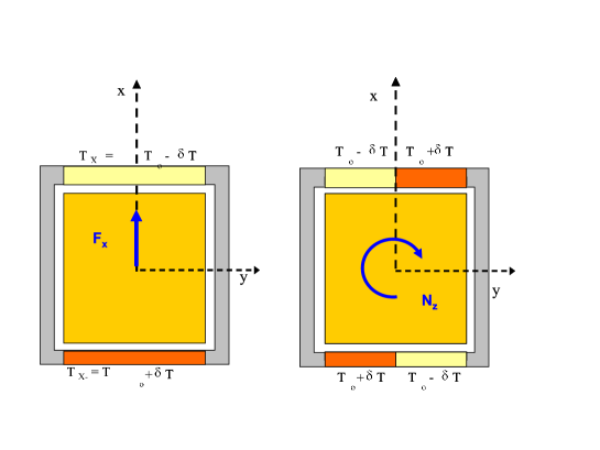
Figure 2: Idealized temperature gradient configurations. The orange square represents a section of a cubic TM of size L at uniform temperature $T_{0}$. Yellow and red parts represent domains of uniform temperature on the inner surface of the electrode housing, as indicated next to them. Left panel: because of radiometer effects (and, as shown in Sec. II.2, radiation pressure), the illustrated temperature pattern is expected to induce a net force $F_{x}$. Right panel: the illustrated temperature pattern is expected to induce a torque $N_{z}$ around the TM $z$ axis. In the simplified infinite plate model of the radiometer and radiation pressure effects, the gray parts of the electrode housing do not contribute to $F_{x}$, even in the presence of a temperature gradient (see Eqn.3). The gray part can, in this simplified model, contribute to $N_{z}$, in the event of a thermal gradient, through the forces that they cause orthogonally to the TM faces in front of them (as in Eqn.5).

By analogy with the correction factor $\kappa_{R}$ introduced in Eqn.4, we include here the factor $\gamma_{R}$, as a radiometric torque correction factor for a finite size sensor. $\gamma_{R}$ will also be a function of the sensor geometry and of the particular temperature distribution inside the sensor that produces a given thermal integral.

To illustrate the significance of the “thermal integral,” we consider the simple temperature distribution on the right in Fig.2, which is an idealization of the temperature pattern imposed in our experiment. In this case,

$$\int_{S}T(\mathbf{s})b(\mathbf{s})ds=\delta T\frac{L^{3}}{2}=4\delta T\frac{L^{2}}{2}\frac{L}{4}\,.$$ (7)

Each “electrode” (the half surfaces of the $X$ faces) contributes with a torque proportional to the temperature difference $\delta T$ multiplied by its area $L\times\frac{L}{2}$ and the ”arm” $\frac{L}{4}$ (that is the distance of the center of the electrode from the center of the TM face). For the same $\delta T$, the thermal integral scales as the cube of the linear size of the TM.

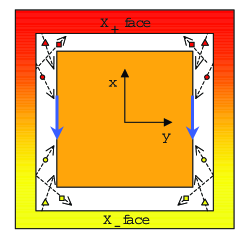
Figure 3: Cartoon of the GRS cross section, illustrating shear forces along $x$ caused by molecules striking the $Y$ TM faces in the presence of a linear thermal gradient in $x$ (as in the simulations of App. A). Molecules striking the $Y$ faces impart shear forces parallel to the TM surface along $x$. For a non-infinite TM, some molecules (such as those represented by squares) emitted from a given point on $Y$ sensor surfaces do not strike the TM. As such, this asymmetrizes the $x$ momentum imparted to the TM by the molecules originating in the given sensor-face location, which, in the presence of a thermal gradient produces a net thermal shear force (blue arrows). This is reinforced by molecules (represented by triangles) starting from the $X$ faces near the corners. From the standpoint of a surface element of the TM, there is a net imbalance in the shear momentum imparted by the molecules arriving from the hot (red) and cold (yellow) sides that contributes to the overall translational radiometric effect. This shear effect increases with increasing gap size.
Note that the momentum components transferred normal and parallel to the $Y$ surface contribute to the torque around the $z$ axis with opposite sign. As such, these shear forces are also responsible for a reduction in the radiometric torque, relevant to the experiments presented here.

For realistic sensor dimensions, finite size effects begin to erode the infinite plate assumptions used here. First, not all molecules leaving the GRS surface directly in front of the TM (for the $X$ faces, the yellow and red zones in Fig.2) strike the TM. Other molecules originating in the corners (the grey corners in Fig.2) do strike the TM, on the $X$ faces but also on the $Y$ and $Z$ faces. Additionally, molecules striking the $Y$ and $Z$ faces impart shear forces along $x$, which in the presence of a temperature gradient is rendered asymmetric by the finite TM dimension (illustrated in Fig.3). These phenomena are enhanced with larger gaps and, in connection with temperature-induced asymmetry of the molecular velocity distribution, are expected to contribute to both $F_{Rx}$ and $N_{Rz}$. To understand the role of these corrections to the simple radiometric model presented above, we have performed a numerical gas dynamics simulation, which is described in detail in App. A.

Simulations have been performed for a cubic 46 mm TM inside a rectangular box, with several different gap sizes, including the geometry for the LISA Pathfinder sensor design (shown in Fig.1). The simulations consider a temperature difference $\Delta T_{x}$ constituted by $X_{+}$ and $X_{-}$ faces that are at constant temperature (differing by $\Delta T_{x}$), with a linear temperature gradient along the $Y$ and $Z$ faces (as illustrated in Fig.3). For the TM force along $x$, the simulations indeed verify the simplified model of Eqn.4 ($\kappa_{R}=1$), to within 10%, for the smallest TM-GRS gaps studied (1 mm, see Fig.13 in App. A), with the force coming nearly exclusively from molecules impacting the $X$ faces. With increasing gap size, however, the calculation demonstrates the role of shear forces along the $Y$ and $Z$ faces, which contribute to an excess of roughly 40 % above the infinite plate model prediction for the largest gaps of the study (7 mm). For the LISA Pathfinder GRS design, the radiometric force transfer function $\left.\frac{dF_{x}}{d\left(\Delta T\right)}\right|_{R}$ exceeds the infinite plate prediction Eqn.3 by roughly 25 % ( $\kappa_{R}\approx 1.25)$, with a statistical error of several percent (results are summarized in Table 1, along with those from a similar radiation pressure simulation).

$\kappa_{R}$		1.25
	$a$ = 1	1.17
$\kappa_{RP}$	$a$ = 0.05 (specular)	0.32
	$a$ = 0.05 (diffuse)	0.75

Table 1: Results of the thermal gradient simulations, where $\kappa_{R}$ and $\kappa_{RD}$ represent correction factors to the infinite plate model for, respectively, the radiometric effect (Eqn.4) and differential radiation pressure (Eqn.10). The simulations assume the LTP GRS design geometry and a temperature difference between two opposing GRS $X$ faces, each at a uniform temperature and with a linear temperature gradient along the $Y$ and $Z$ faces. Results for radiation pressure are shown for different values of the absorption $a$ and nature of reflection (specular or diffuse). Statistical errors are of order several percent.

The simulations employing a linear temperature gradient along $x$ also allow an estimate of the radiometric torque relevant to the torsion pendulum experiment, as the linear temperature profile along $y$ produces a torque around the $z$ axis. Here, a net decrease of the radiometric effect is observed with respect to the simplified model of Eqn.5 (see Fig.13 of App. A). With increasing gap, there is a suppression of the radiometric torque, dominated by the same shear forces mentioned above, which tend to work against the torque contribution of the dominant normal component of the molecular impacts (illustrated in Fig.3). The magnitude of the torque reduction, with respect to the infinite plate model, is in fact roughly consistent with the shear force -relevant to the increase in radiometric force reported above -multiplied by an arm length of $L$/2, or half the TM width. For the $Y$ face torque contribution for the 2 mm gap sensor, we find roughly 83% of the torque calculated with the infinite plate model (Eqn.5), and only 65% for the larger-gapped LTP GRS prototype.

The true correction factor $\gamma_{R}$ will depend on the real temperature profile for the experiment, rather than the contribution of a single face that sees a linear temperature profile. However, the experimental uncertainty in estimating the true temperature profile in these experiments (see Sec. III.3 and App. C), particularly in the corners of the sensor where the finite-size corrections are most relevant, limits the value of a simulation performed with a “full” (but very approximate) sensor temperature distribution. A linear temperature distribution also turns out to be a decent approximation for the experimental temperature distributions. As such, the torque results obtained for a linear temperature gradient, extrapolated to a full sensor, yield indicative estimates, $\gamma_{R}\approx 0.65$ and $\gamma_{R}\simeq 0.8$, for comparing the experimental results for the torque measurements for, respectively, the LTP GRS and 2 mm sensor prototypes.

II.2 Thermal Radiation Pressure

The effect of thermal radiation pressure can be evaluated from the momentum transfer of thermal photons emitted by all radiating surfaces inside the GRS. We again assume an infinite parallel plate approximation, in which all thermal photons wind up being absorbed in the vicinity of emission, either on the parallel surface opposite the point of emission or reflected back onto the original emitting surface. Assuming the same emissivity for all the involved surfaces, each surface element $d\mathbf{s}$ on the internal TM-facing surfaces of the sensor contributes with a force $dF_{RP}(\mathbf{r})$ acting on the TM in the direction perpendicular to the surface element itself. This force is given by

$$dF_{RP}(\mathbf{r})=\frac{2\sigma}{3c}T^{4}(\mathbf{r})d\mathbf{s}\simeq\frac{2\sigma}{3c}T_{0}^{4}(\mathbf{r})d\mathbf{s}+\frac{8\sigma}{3c}T^{3}_{0}\delta T(\mathbf{r})d\mathbf{s}$$ (8)

with $\sigma$ the Stefan-Boltzmann constant and $c$ the speed of light. Assuming that the TM is isothermal, and thus contributes no net recoil force from its radiation, the net force acting on the TM in the sensitive $x$ direction for LISA will be proportional to the average temperature difference between opposing sensor faces, given by

$$F_{RP_{x}}\simeq\mathrm{A}\frac{8\sigma}{3c}T^{3}_{0}\left(\overline{T}_{X_{+}}-\overline{T}_{X_{-}}\right).$$ (9)

where Eqn.8 is integrated over the EH surfaces that directly face the TM (the yellow and red zones in the left image in Fig.2). Thus, the radiation pressure transfer function can be expressed

$$\left.\frac{dF_{x}}{d\left({\Delta T}_{x}\right)}\right|_{RP} \simeq \kappa_{RP}\mathrm{A}\frac{8\sigma}{3c}T^{3}_{0}$$ (10)

$$\simeq 27\>\mathrm{pN/K}\times\kappa_{RP}\left(\frac{T_{0}}{293\>\mathrm{K}}\right)^{3}.$$

As in Sec. II.1, we can integrate the moment of the force element $dF_{RP}$ (Eqn.8) to calculate the torque $N_{z}$,

$$N_{RPz}\simeq\gamma_{RP}\frac{8\sigma}{3c}T_{0}^{3}\int_{S}T(\mathbf{s})b(\mathbf{s})ds.$$ (11)

where both the $X$ and $Y$ faces contribute. We note that in analogy with the radiometric effect in the previous section, we have introduced, in Eqns. 10 and 11, respectively, we have introduced the radiation pressure force and torque factors $\kappa_{RP}$ and $\gamma_{RP}$, to account for corrections due to the inaccuracy in applying this simple infinite plate model to our true sensor geometry.

As with the radiometric effect, the assumptions for this simple radiation pressure model begin to break down when the gap sizes are not negligible compared to the TM dimensions. Just as for gas molecules, there are corrections due to emitted photons “missing” the TM and hitting adjacent faces, as well as adsorbed photons along the lateral ($Y$ and $Z$) faces imparting a shear force and associated torque on the TM. In addition, the presence of finite reflectivity (absorptivity $a<1$ means that bouncing thermal photons will hit multiple surfaces, imparting force and torque components with different signs, before adsorbing. This latter effect is particularly significant for the metallic surfaces inside the sensor, which are expected to have a high 90-95 % reflectivities ($a\approx 0.05-0.1$) at thermal photon wavelengths radiaprop , and systematically serves to homogenize the radiation pressure felt by the TM, suppressing the differential radiation pressure effect.

To properly analyze such effects, a numerical simulation was performed and is described in detail in Sec. B. The simulation studied several representative simplified sensor geometries and sensor temperature profiles representative for the force for LISA and for the torque relevant to the experiments presented in the following sections. Additionally, different extreme cases for the infrared absorption $a$ and for the nature of the reflection (specular or diffuse) were considered. For the force, a simple linear temperature gradient along the $x$ axis was assumed, with uniform temperature across each $X$ face. In the limit of vanishing TM-sensor gaps (0.2 mm), the infinite parallel plate model for the force (Eqn.9) was confirmed, with the factor $\frac{8\sigma}{3c}$ (or $\kappa_{RP}\approx 1$), to within several percent, even for absorption as small as 0.1. For perfect absorption ($a$ = 1), there is an increase in the radiation pressure effect akin to that for the radiometric effect, with $\kappa_{RP}=1.17$ for the LISA Pathfinder geometry (see the summary of results in Table 1). For the case of the high reflectivity surfaces expected for the LISA sensor – using $a=0.05$, with specular reflection – there is a suppression of the effect, with $\kappa_{RP}=0.32$. This result thus indicates a significant, if not order-of-magnitude, change to the estimate of the effect given in simplified radiation pressure models for LISA Stebbins et al. (2003); Schumaker et al. (2003); Dolesi et al. (2003).

For the torque, assuming temperature profiles similar to that estimated in our experiments (using the technique described in Appendix A), the suppression of the differential radiation pressure effect is more pronounced, with photons moving, in only a couple bounces, from one half of the TM to the other (or to an adjacent face), inverting the sign of the resulting torque. For the high reflectivity surfaces ($a=0.05$ and specular reflection) reasonable for the gold coated TM and sensors used, we obtain radiation pressure torque correction factors $\gamma_{RP}$ of order 0.4 and 0.3 for the 2 mm and 4 mm (LISA Pathfinder design) prototypes used in the experiment. This significant reduction has an impact on the interpretation of the experimental results discussed in Sec. IV.

II.3 Asymmetric temperature dependent outgassing

Outgassing of molecules absorbed by the internal walls of the GRS increases the residual pressure surrounding the TM. Additionally, an asymmetry in the molecular outflow can be created or enhanced by the temperature dependence of the outgassing, resulting in a differential pressure that is driven by the GRS temperature gradient itself.

As asymmetric outgassing depends on the amount and type of absorbed impurities inside the GRS, it is a contamination effect that does not lend itself easily to a first principles calculation, in contrast with the previous two effects. However, the gas flow from a surface can be modelled with a temperature activation law $\mathcal{Q}(T)=\mathcal{Q}_{0}e^{(-\Theta/T)}$, where $\mathcal{Q}_{0}$ is a flow prefactor and $\Theta$ the activation temperature of the molecular species under consideration rudiger ; big . Our simplified model considers only a single outgassing species which is uniformly desorbed from identical GRS surfaces, and that the molecules emitted from the sensor walls collide with the TM without sticking. A temperature gradient $\Delta T_{x}$ would induce an asymmetric rate of outgassing across the TM $\Delta\mathcal{Q}(T)\approx\mathcal{Q}(T_{0})\left(\Theta/T_{0}\right)\left(\Delta T_{x}/T_{0}\right)$. The consequent difference in pressure $\Delta P_{out}$ across the TM would cause a force $F_{OGx}$ given by

$$F_{OGx}=A\,\Delta P_{OG}=A\frac{\Delta\mathcal{Q}(T)}{C_{eff}}\approx A\frac{\mathcal{Q}(T_{0})}{C_{eff}}\frac{\Theta}{T_{0}}\frac{\Delta T_{x}}{T_{0}}$$ (12)

where $C_{eff}$ is a geometrical factor resulting from a combination of the conductance of the paths around the TM and through the holes in the GRS electrode housing walls, estimated to be roughly 4.3 $\times 10^{-2}$ m³/s for the LISA / LISA Pathfinder GRS geometry Dolesi et al. (2003). The asymmetric outgassing transfer function is then given by

$$\left.\frac{dF_{x}}{d\Delta T}_{x}\right|_{OG} \simeq A\frac{\mathcal{Q}(T_{0})}{C_{eff}}\frac{\Theta}{T_{0}^{2}}$$ (13)

$$\simeq 40\,\frac{pN}{K}\left(\frac{\mathcal{Q}(T_{0})}{1.4\,\mathrm{nJ/s}}\right)\left(\frac{\Theta}{3\times 10^{4}\,\mathrm{K}}\right)\left(\frac{293\,\mathrm{K}}{T_{0}}\right)^{2}$$

We note that the temperature dependence of the effect, partially hidden in $Q(T_{0})$, is $\frac{1}{T^{2}}\exp{\left(-\Theta/T\right)}$, at least in this simplified model with a single outgassing species, and is thus a rapidly increasing function at the temperatures of our study. The values used for the flow $\mathcal{Q}(T_{0})$ and the activation temperature $\Theta$ correspond to typical room temperature behaviors for the metal and ceramic materials used in the GRS Roth:book ; hanlon:book . This source of coupling to the thermal gradient thus appears to be roughly equal in magnitude to that of the combined radiometric and radiation pressure effects (Eqns. 4 and 10). However, given the likely large variability due to materials, assembly, cleaning, and thermal history of the sensor, this noise source has a much larger uncertainty and is a key motivation for measurement of the overall thermal gradient transfer function. If the outgassing phenomenon were indeed uniform across the GRS surfaces, the torque transfer coefficient could be found by integrating the moment due to the differential outgassing pressure over the sensor surfaces, as for the two preceding thermal gradient effects. This would allow conversion between force and torque through an effective arm length, of order $\frac{L}{4}$ for a simplified temperature distribution like that in Fig.2. However, unlike the previous two effects, the numerous features in the sensor – holes, interfaces between the metal and ceramic surfaces – suggest that the outgassing could be concentrated in specific localized areas, rather than uniform. As such, there is no simple, unequivocal extrapolation of $\left.\frac{dF_{x}}{d\Delta T_{x}}\right|_{OG}$ from a torque measurement. However, the torque measurements are sensitive to nearly all possible outgassing effects, regardless of their model, and the lack of a significant excess beyond the well-modelled radiometric and radiation pressure effects will certainly build confidence that there is no dominant asymmetric outgassing effect for LISA.

III Experimental Details

III.1 Gravitational Reference Sensor prototypes

This experimental campaign studied two GRS prototypes realized as part of the sensor design development for LISA. They feature different electrodes geometries, construction techniques, and TM sizes. Both sensors are based on a Gold coated Molybdenum housing, with insulating elements made from the Aluminum-based, high thermal conductivity ceramic SHAPAL. The first prototype sensor, referred to here as “TN2mm” uses a 40mm cubic TM, with a gap – the distance between the TM and the surrounding electrode and electrode housing surfaces – of 2 mm, symmetric on all three axes. The electrodes are Au-coated bulk Mo plates separated from the grounded housing by bulk Shapal plates. The second prototype, “EM4mm,” reflects the final GRS design for the LTP mission, with a 46mm cubic TM and gaps of 4, 2.9 and 3.5  mm on, respectively, the $x$, $y$, and $z$ axes (see Fig.1). In contrast with TN2mm, the electrodes for EM4mm are obtained by Au sputtering deposition directly on the bulk insulating SHAPAL plates.

III.1.1 Electrical heaters and thermometers

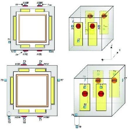
Figure 4: Top panel: prototype TN2mm was equipped with five thermometers and the experiment was performed by alternatively switching on and off the heaters H1E and H1W (red circles). Bottom panel: prototype EM4mm, equipped with eight thermometers. For prototype EM4mm we employed all four heaters, alternatively switching the pairs (H1E,H2W) and (H2E,H1W). We note that $T_{fake}$ is included here on the TN2mm $X+$ face to indicate the position of a temperature reading that, as described in App. C, has been artificially added to help estimate the temperature profile, in the absence of a thermometer near to heater H2W.

Electrical heaters have been installed on the external surfaces of both sensor prototypes, in correspondence with the $X$ face electrodes. They are displaced with respect to the pendulum torsion axis (see Fig.4) and can thus apply the rotational temperature differences that convert the forces described in Sec. II into torques, to which this pendulum is sensitive. The heaters are made from of twisted pairs of Manganin wires several meters long, wound onto 5 mm diameter Al cylinders. The heaters are attached to the sensor with a high thermal conductivity, vacuum compatible glue, for the TN2mm prototype, and tightly screwed onto the GRS surfaces for EM4mm. The resistance of each heater is $95\pm 1$ Ohms. A 1 Hz square wave voltage, up to a maximum of 7 V across the resistor (nearly 0.5 W), is supplied to the heaters with high output current operational amplifiers. Twisting the heater wires limits the magnetic field produced by the heater current, and the use of the 1 Hz square wave allows application of constant heater power, while at the same time converting any residual magnetic field-related torque to a frequency well above our measurement frequency of 0.4-0.5 mHz (see Sec. III.3).

With the aim of reconstructing the temperature profile of the GRS, temperatures at different positions are measured for each sensor, by a set of Pt100 thermometers on the electrode housing external surfaces. They are glued to the sensor by means of a high thermal conductivity vacuum compatible glue. Five thermometers were used on the TN2mm prototype and eight on EM4mm. A sketch of the thermometer and heater locations is shown for both sensors in Fig.4.

III.2 Torsion pendulum apparatus

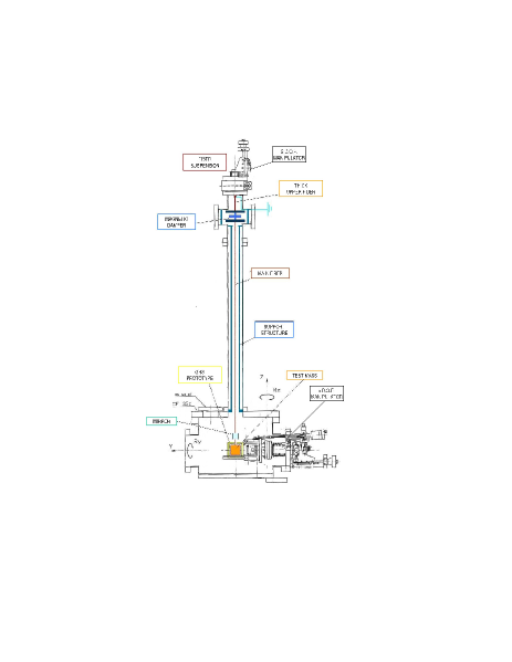
Figure 5: Schematic of the torsion pendulum apparatus. The TM is the main part of the inertial member of a torsion pendulum hanging from a long torsion fiber designed to have the minimum stiffness and thus the maximum sensitivity. The electrode housing surrounds the TM and is attached to a precision positioner that can center it relative to the TM in 6 degrees of freedom.

This experimental investigation has been performed with a torsion pendulum facility Hueller et al. (2002); Carbone et al. (2007, 2003, 2003); carbone:thesis ; Carbone et al. (2005), where a representative copy of the LISA test mass is suspended by a thin fiber and hangs inside a prototype of the GRS. The small torsional elastic constant of the fiber allows for high resolution measurement of torques around the fiber axis, via measurement of the pendulum angular deflection. Measurements of the pendulum angular deflection noise can be used to study the force noise acting on the LISA TM. Additionally, controlledly modulation of known disturbance fields, such as the thermal gradients in this study, with coherent detection of the resulting pendulum deflection, can allow a study of known force noise sources relevant to LISA free-fall.

The pendulum is designed for minimum elastic stiffness and thus maximum torque sensitivity. A light-weight hollow TM (Au-coated Ti for TN2mm, and Au-coated Al for EM4mm) has been chosen to maximize the torque sensitivity, allowing use of a thin (25 $\mu$m) tungsten fiber, with a resulting resonant frequency near 2 mHz and quality factor near 3000. The pendulum and sensor are mounted on independent micro-positioners, allowing a 6 degree of freedom adjustment of the relative position of TM inside the electrode housing. The torsion pendulum deflection angle was read out, with 10 Hz sampling rate, by an optical autocollimator measurement of a mirror that was part of the torsion member.

The vacuum chamber that accomodates the pendulum and the GRS is evacuated by means of a turbomolecular pump, and its pressure is monitored by means of an ionization gauge (Varian UHV 24). The whole apparatus sits in a thermally controlled room with 50 mK long term stability.

The pendulum torque resolution relevant to these measurements is typically 5-10 fN m / Hz^1/2 near the 0.4 - 0.5 mHz heater power modulation frequency, which is a factor 2-3 above the Brownian thermal noise limit for the pendulum. For the several hour integration times used in these measurements, this equates to a torque resolution of order 0.1 fN m.

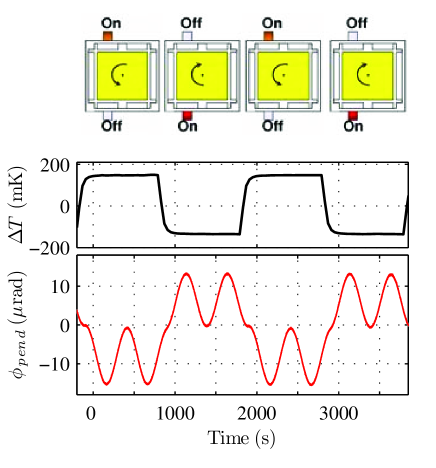
Figure 6: Illustration of the thermal gradient effects measurement technique for the the TN2mm prototype. Here 200 mW are alternatively applied to heaters (H1E and H1W in Fig.4) located off-axis on opposing sensor faces, switching at 1000 s intervals (top panel). The central panel shows the induced temperature difference $\Delta T=\left(T_{2}-T_{4}\right)$. The resulting thermally induced torque causes the pendulum to respond coherently, as shown in bottom panel, with an angular deflection at the heater modulation frequency superimposed on the pendulum free oscillation.

III.3 Measurement technique and data analysis

The general experimental technique, illustrated in Fig.4, is to create an oscillating asymmetric temperature distribution by modulated heater powers and then measure the resulting coherent oscillations both in the torque on the TM and in the GRS temperature distribution. Varying and monitoring the average sensor temperature and pressure, in addition to the oscillating temperature difference pattern, allows separation of the different thermally induced torque effects for their dependence on these parameters. In presenting the measured torque data, they will be normalized for the amplitude of the applied temperature gradients as expressed by the estimated applied “thermal integral,” the integral $\int_{S}T(\mathbf{s})b(\mathbf{s})ds$ introduced in Sec. II to characterize the radiometric and radiation pressure torques in the infinite plate limit. This normalization allows comparison between measurements of different thermal gradient amplitudes and comparison with the models for the radiometric and radiation pressure effects discussed in Sec. II.

III.3.1 Rotational thermal gradients: application and estimation

For the TN2mm prototype, the oscillating temperature pattern were obtained by alternately switching on and off two opposing heaters for 1000 s, as illustrated in Fig.4. For the EM4mm prototype, two pairs of opposing heaters are switched on and off for 1250 s. These modulation frequencies, 0.5 and 0.4 mHz respectively, result in coherent pendulum torques that are below the roughly 2 mHz resonant frequency. Typical peak to peak temperature differences across the sensor ranged from tens to hundreds of mK. The alternate switching of the heaters produce an oscillating temperature gradient pattern across the EH, with the time dependence of a lightly filtered square-wave. We note that the thermal time constant for equilibration across the GRS, relevant to the temperature difference (as plotted in Fig.4) and to the thermal integral, is of order 100 s.

The temperature pattern was recorded in the readings $T_{i}(t)$ of each thermometer $i$ at its position $(s_{1},s_{2})_{i}$, where $s_{1}$ and $s_{2}$ are the two coordinates mapping the 4 $X$ and $Y$ GRS surfaces. For each cycle $k$ of the heater power modulation, we calculate the component $T(s_{1},s_{2},\omega,k)_{i}$ of $T_{i}(t)$ at the modulation carrier frequency and at its third and fifth harmonics, where the filtered square wave thermal pattern is known to have significant spectral content. An estimation of the components $T(s_{1},s_{2},\omega,k)$ at a generic position $(s1,s2)$ was then obtained by spatial interpolation of the values $T(s_{1},s_{2},\omega,k)_{i}$ (for details see the appendix App. C). For each demodulation cycle $k$, it was then possible to obtain an estimation of the $\omega$ component of the “thermal integral”, as defined in Eqn.5 and

$$\left(\int_{S}T(s)b(s)ds\right)_{(\omega,k)} =\sum_{X_{+},X_{-}}\int_{A}(\pm)T(y,z,\omega,k)ydydz+$$ (14)

$$+ \sum_{Y_{+},Y_{-}}\int_{A}\left(\mp\right)T(x,z,\omega,k)xdydz$$

As discussed in appendix App. C, our analysis shows that the simple interpolation technique used underestimates the thermal integral, by 20-30 % in the simplified analysis used. However, given the coarse sampling of the temperature distribution with only 5-8 thermometers and the approximate nature of the analysis used, we have chosen not to “correct” the data presented for this systematic error, but rather to present the data obtained from the relatively straightforward interpolation. The uncertainties in the estimation of the thermal integral are of order 20% and 50% for, respectively, the EM4mm and TN2mm sensors. Given the repeated use of the same heating pattern for each of the two sensor datasets, the uncertainty in the thermal integral estimation can be thought of a single scale factor for each dataset.

III.3.2 Torque estimation

The thermal gradient induced torque on the TM is detected in the coherent deflection of the pendulum. The torque components are calculated for each cycle $k$, at the odd harmonics of the heater power modulation frequency, using the torsion pendulum transfer function, as in Refs. Carbone et al. (2003) and Carbone et al. (2005). The resolution of order 0.1fN m obtained for a several hour integration corresponds to a signal-to-noise ratio of order 10 for the smallest thermal gradient-induced torques measured.

The torque data for each cycle are normalized by division by the calculated thermal integrals,

$$N^{*}_{(\omega,k)}=\frac{N_{(\omega,k)}}{\left(\int_{S}T(s)b(s)ds\right)_{(\omega,k)}}$$ (15)

The units of $N^{*}_{(\omega,k)}$ are $\frac{Pa}{K}$.

III.3.3 Average temperature: control and estimation

Average temperatures between 283 K and 314 K were obtained by changing the temperature of the room containing the pendulum apparatus and by changing the total DC power applied to the heaters. The average temperature of the electrode housing and TM $T_{0}$ is derived by averaging the thermometer data for each measurement cycle. In particular, average temperature data for UTN2mm were obtained with $T_{0}=\frac{T_{2}+T_{4}}{2}$, whereas for EM4mm we used $T_{0}=\frac{T_{1}+T_{2}+T_{3}+T_{4}}{4}$ (see Fig.4.

III.3.4 Average pressure: control and estimation

The pressure in the vacuum enclosure were set to different equilibrium levels, from roughly $2\times 10^{-6}$ Pa to $10^{-4}$ Pa, by changing the conductance between the vacuum vessel and the pumping system. The pressure in the vacuum vessel was measured by an ionization gauge (Varian UHV 24), sampled at 1 Hz and averaged for each cycle of the heater modulation. The calibration of the ion gauge, for which no certification was available, was obtained by testing against a similar device (Pfeiffer UHV), that was certified by the manufacturer to within 15$\%$. It was not possible to use the Pfeiffer gauge constantly because of its very high filament current, which produced an intolerable electrostatic charging of the TM. The calibration was performed by simultaneously acquiring both gauges while slowly changing the pressure in the vacuum vessel with a valve on the pumping line, over a pressure range from roughly $5\times 10^{-6}$ Pa up to $2\times 10^{-4}$ Pa, roughly the same range spanned by our study. The resulting fit of the obtained curve was applied to calibrate the Varian gauge in all measurements.

IV Experimental Results and Discussion

Results of the experimental investigation for both the TN2mm and EM4mm sensors are shown in Fig.7, where we report $N^{*}_{(\omega,k)}$, the component of the normalized torque at the heater modulation carrier frequency $\omega$, as a function of pressure and for several average sensor temperatures. The data are dominated by the linear pressure dependence of the radiometric effect, which will be discussed in the following paragraphs.

In Fig.8 we plot the normalized torque data at the first, third, and fifth harmonics of the modulation frequency (0.4, 1.2 and 2.0 mHz) – each normalized for the thermal integral at the relevant frequency – with the 298.9 K data for the EM4mm sensor chosen as an example. The data at the three frequencies are equivalent within the statistical errors of the measurement. In this study, no frequency dependence in the transfer function between measured thermal gradients and resulting torque has been observed. Also, by varying the amplitude of the modulated heater power, we can check the linearity of the thermal induced torque effects in the applied thermal integral amplitudes. One example is shown in Fig.9 for the prototype TN2mm, showing that the normalized torque data are reproduced, within the statistical errors, for the two different temperature gradient amplitudes. These two observations confirm the linear, frequency-independent nature of the thermal gradient torque models discussed in Sec. II.

In the following two sections we discuss the experimental results in light of the models for the radiometric, radiation pressure, and temperature-dependent outgassing effects discussed in Sec. II. From Eqns. 6 and 11, we expect that

$$N^{*}_{(\omega,k)}\simeq\gamma_{R}\frac{P}{4T_{0}}+\gamma_{RP}\frac{8\sigma}{3c}T_{0}^{3},$$ (16)

with an additional pressure independent term coming from temperature-dependent outgassing. By fitting the data for $N^{*}\left(T_{0},P\right)$ in Fig.7 to the linear pressure dependence at each average GRS temperature $T_{0}$, we first study the radiometric effect, through the pressure slope. Finally through the zero-pressure intercept, we can study the radiation pressure effect and any outgassing related phenomena.

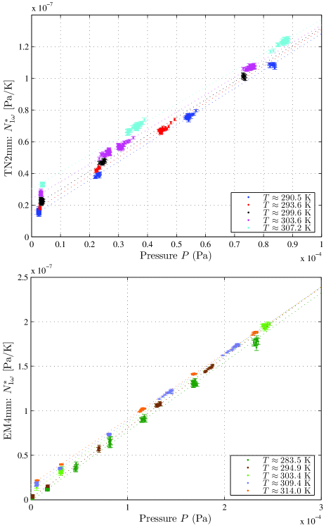
Figure 7: Normalized torque $N^{*}_{(\omega,k)}$ of Eqn.15, as a function of pressure at different average temperatures. Top panel the data for TN2mm prototype sensor, the bottom panel the data for GRS Engineering Model for the LTP , indicated with EM4mm. Dashed lines are the results of linear least square fits to the pressure at each average temperature. Only data for the first harmonic of the excitation frequency are shown.

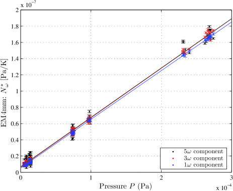
Figure 8: Normalized torques $N^{*}_{\omega,k}$ as function of the residual pressure $P$, at the average temperature $T_{0}\approx 298.9$K, calculated at the fundamental frequency $1\omega=0.4$mHz (blue dots) and its odd harmonics $3\omega=1.2$mHz (red) and $5\omega=2$mHz (black) (data for the EM4mm sensor). Linear fits also are shown for comparison. The three measured slopes and the three intercepts agree with each other within their statistical errors (smaller than $4\%$).

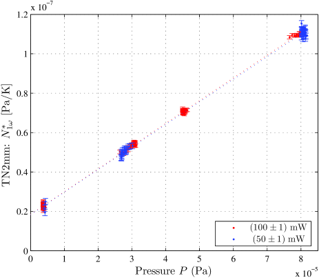
Figure 9: Measurement of $N^{*}_{(\omega,k)}$ as a function of pressure, with prototype TN2mm, for different values of applied heat. Red points: alternating $200\pm 2$ mW between heaters H1E and H1W. Blue points: apply $50\pm 1$ mW continuously to both heaters and alternating $100\pm 1$ mW. Lines are best fits to data.

IV.1 Comparison with the radiometer effect model

According to Eqn.16, for the radiometer effect $N^{*}(\omega,k)$ should depend linearly on pressure with a slope given by

$$\left(\frac{\partial N^{*}_{\omega}}{\partial P}\right)_{T_{0}}=\frac{\gamma_{R}}{4T_{0}}$$ (17)

where the correction factor $\gamma_{R}=1$ in the limit of the infinite plate model. Fig.7 does indeed show that $N^{*}(\omega,k)$ depends linearly on $P$, with a slope that decreases with $T_{0}$ (barely visible by eye in the plotted data).

In Fig.10, we plot the slope $\left(\frac{\partial N^{*}_{1\omega}}{\partial P}\right)_{T_{0}}$ multiplied by $4\,T_{0}$, which thus represents the measured $\gamma_{R}$, a constant according to our model. The results yield $\gamma_{R}=1.34$ for the TN2mm prototype and $\gamma_{R}=0.92$ for EM4mm. The RMS fit residuals are of order 1.5% for each sensor, resulting in overall uncertainties in $\gamma_{R}$ slightly below 1%. We note that, for both sensors, the observed scatter in these data exceeds that estimated by the statistical torque uncertainty, by a factor 4-8. As such these data are not limited by the torque resolution, but likely by systematic uncertainties in the temperature integral and pressure measurements between points at different temperature. We note that the temperature ranges for both sets of data are sufficient to distinguish the temperature dependence, and the fit to the $\frac{1}{T_{0}}$ model (Eqn.17) is significantly better than a fit to a constant (temperature independent) or to $\frac{1}{T_{0}^{2}}$.

Figure 10 also presents the values for $\gamma_{R}$ calculated in the radiometric simulations for the two sensor geometries, assuming a simplified linear temperature gradient (Sec. A), which yielded $\gamma_{R}=0.83$ for TN2mm and $\gamma_{R}=0.65$ for EM4mm. In comparing the experimentally measured values to these predictions, we have to consider the systematic uncertainties in the estimate of the thermal integral that has been used to normalize the torque data. The temperature interpolation scheme used to estimate the thermal integral, discussed in Appendix C, is likely to underestimate the thermal integral. By one approximate analysis, this underestimate could be roughly $20-30\%$ for the two sensors. Underestimating the thermal integral would systematically increase the values of $\gamma_{R}$ obtained here, effectively scaling each of the two sensor data curves shown here (as each data set relied on a single pattern of heating and thermometer sampling, it is likely that each data set would have a systematic error characterized by a single scale factor). Without a more reliable model for calculating the thermal integral from the limited number of thermometers on the sensor, the data presented use the simple temperature interpolation, with an estimated systematic uncertainty of order $50\%$ and $20\%$ for the TN2mm and EM4mm sensors, respectively. As such, the data for both sensors are consistent with the predictions for the radiometric effect. The uncertainties are however too large to test the radiometric model at a level approaching the statistical resolution of the measurements, or to test definitively the modifications to the infinite plate model predicted by the simulations for the two sensors.

In addition to confirming the model of the radiometric effect, these data confirm, and extend – to a wider range of pressure, temperature, and to a second prototype sensor – our preliminary observations with the TN2mm sensor carbone:thesis ; Carbone et al. (2005). We note that a thermal gradient-induced torque that increases with pressure is also observed in a LISA-related study at the University of Washington (UW) pollack:thermal , for measurements at two pressures and two temperatures. This study, which employed a much simpler and more open geometry than the LISA GRS, observed forces of the same order of magnitude as those observed here. However the authors report an unexpected frequency dependence, which is not observed at all in the measurements presented here. In addition, the UW study reports an increase in the pressure dependent effect with increasing temperature, which is contrary to the expected radiometric $\frac{1}{T}$ dependence observed here. Given the differences in the experimental geometry and the limited number of presented measurements, it is not possible at this time to further discuss these apparent discrepancies.

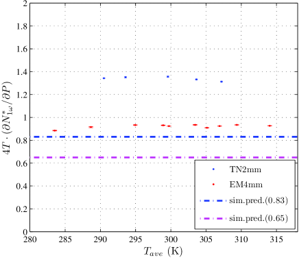
Figure 10: Normalized measured slopes $4T_{0}\frac{\partial N^{*}_{\omega}}{\partial P}$ of the fitting lines in Fig.7 as a function of the average temperatures $T_{0}$ (blue dots: prototype TN2mm; red dots: prototype EM4mm). The results represent measurements of the radiometric correction factor $\gamma_{R}$, which is unity in the infinite plate model. Horizontal dashed lines: values predicted by the simulation for a linear thermal gradient (blue and red refer to TN2mm and EM4mm, respectively) from App. A. We note that the error bars represent only the statistical uncertainties in the torque measurement. The systematic uncertainty in the estimate of the relevant thermal integral is much larger, of order 20% and 50% for the EM4mm and TN2mm prototypes, and serves as an uncertainty in the overall scale factor for each of the two datasets.

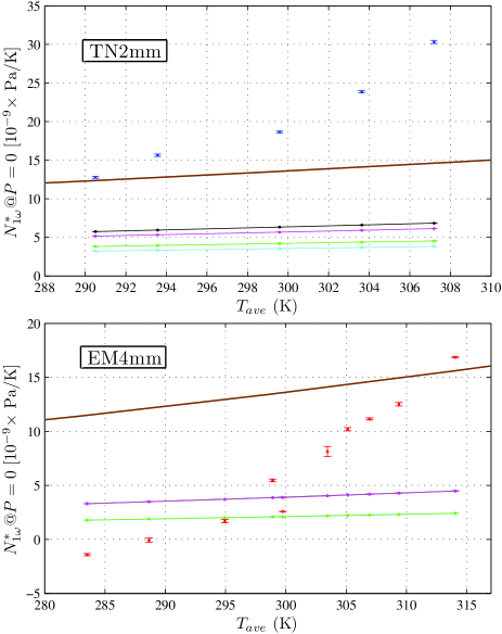
Figure 11: Measured intercepts of the linear fittings of the curves reported in Fig.7. Top panel: data of the TN2mm prototype, represented with blue dots. Bottom panel: data of the EM4mm, represented with red dots. Error bars indicate only the statistical uncertainty in the torque measurements. The lines of the radiation pressure contribution to the intercepts predicted by different models are shown for comparison in both panels. The brown continuous lines show the prediction of the infinite plates approximation ($\frac{8\sigma}{3c}T_{0}^{3}$ as in Eqn.11), which is the same for both sensors. The other models are derived from the numerical simulations discussed in App. B and using the temperature patterns estimated with the procedure described in App. C. Different values have been taken into account for the surface absorptivity $a$, and we indicate with $d=100\%$ the case of diffuse light scattering and with $d=0\%$ the specular light scattering case. Orange line: $a=100\%$, $d=0\%$. Black: $a=10\%$, $d=100\%$. Magenta: $a=10\%$,$d=0\%$. Green: $a=5\%$, $d=100\%$. Cian: $a=10\%$, $d=0\%$.

IV.2 The zero pressure limit: thermal radiation pressure and the effect of outgassing

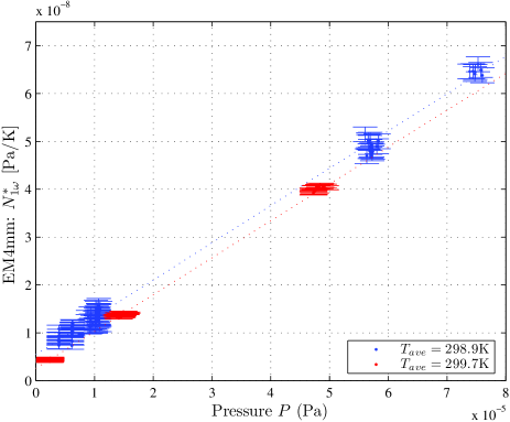
Figure 12: Two measurements of the thermal induced normalized torque for the EM4mm sensor as a function of pressure, at roughly the same average temperature (blue 298.9 K, red 299.7 K) After the first measurement (blue), the sensor temperature was progressively increased to 314 K (highest temperature in Fig.7) while measuring at the higher temperatures of the study. The second (red) data set was measured subsequently after cooling to 299.7 K. The slopes agree within the measurement uncertainty after correction for the small temperature difference. The measured intercept, on the other hand, is reduced by more than a factor 2 in the second measurement, indicating a sharp reduction of the outgassing effect during the “bakeout” at 314 K.

In Fig.11 we plot the zero-pressure values of the normalized torques, $N^{*}(P=0)$, extrapolated to $P=0$ from the data in Fig.7, as a function of the average temperature for the two sensors. Shown for comparison are different estimates of the radiation pressure contribution. These estimates, evaluated for the experimental temperature distributions as estimated in Appendix C, include the infinite plate model of Eqn.11 (brown), and the results of the radiation pressure simulation presented in Sec. B) for 5% absorption and both diffuse (green) and specular (cian) reflection. As discussed in Sec. B, for the geometries of these GRS prototypes, the expected thermal radiation effect is substantially suppressed, relative to the infinite plate prediction, a suppression that is enhanced with increasing reflectivity. Reflectivities of 95 % ($a=0.05$) or higher are in fact expected for gold coating at reflectivity thermal radiation wavelengths radiaprop . While the data for the TN2mm are consistent with the presence of the radiation pressure effect, the data for the EM4mm prototype dip slightly below even the 95% reflection prediction for the radiation pressure effect at the lowest temperatures. This discrepancy will be addressed shortly.

For both sensors, we observe an increase in the zero-pressure torque intercepts with temperature, as expected both for the radiation pressure and outgassing effects. However, for both sensors, the observed increase with temperature is clearly faster than the $T^{3}$ dependence expected for radiation pressure, regardless of the surface reflection properties or geometry, and suggests the exponential-like dependence expected for outgassing. Further evidence for the existence of outgassing-related phenomena is found in the hysteretic behavior of the intercept following a thermal cycle (see Fig.12). This shows that even a mild “bakeout” at 314 K suppresses the intercept near 299 K by more than a factor two, a hysteresis that must reasonably be associated with the degassing of the surface at warmer temperatures.

While outgassing is thus the main effect contributing to the zero pressure data, we note that the its magnitude near 293 K is, for the TN2mm prototype, only roughly equal to that calculated for the infinite plate model for the radiation pressure effect and, for the EM4mm sensor designed for LISA Pathfinder, considerably smaller. As such, the outgassing effect as measured here does not pose a significant increase to the thermal gradient noise budget already considered for LISA.

Even if radiation pressure plays a negligible role in the zero-pressure torque, no simple model can explain the observation that, for the EM4mm prototype, the extrapolated zero-pressure intercept of the normalized torque becomes negative at the lowest temperatures studied. This small – roughly 15% of the magnitude of the infinite plate prediction for the radiation pressure effect – but statistically significant violation of the expected sign for a thermal gradient induced torque is visible in the 283 K data point in Fig.11. There are several possible explanations for this observation:

• Pressure offset If the ion gauge pressure measurements were higher, by a constant offset $P_{OFF}$, than the actual pressure inside the sensor, then the estimated zero-pressure torque intercepts would be artificially lowered. This hypothesis is at least consistent with the fact that, in spite of the fitted negative zero-pressure torque intercepts, we do not observe negative torques even at the lowest measured pressure values. $P_{OFF}$ would have to be roughly $2\times 10^{-6}$ Pa to explain the observed negative torque offset. Given the quoted accuracy of the Pfeiffer gauge, this offset should not exceed $1.5\times 10^{-6}$ Pa (15% of the $10^{-5}$  Pa full scale used for the low pressure data). Such a pressure measurement offset could thus explain most, but not all, of the observed negative torque intercept. Another, slightly less stringent, upper limit on $P_{OFF}$ comes from the lowest pressure measured in the study, $2.3\times 10^{-6}$ Pa.

  We also note that an offset arises in the outgassing from inside the sensor, which causes the true pressure inside the sensor to exceed that measured in the vacuum chamber. This thus has the wrong sign to explain the measured negative zero-pressure torques. Additionally, this effect is estimated to be quite small; given the effective impedance of the holes connecting the sensor to the rest of the vacuum chamber, the pressure inside the sensor would be only 10^-6 Pa higher than outside, even if as much as 10% of the total measured apparatus outgassing (roughly $3\times 10^{-6}$ mbar l / s) originates inside the GRS.

• Inhomogeneous outgassing Outgassing, associated with contamination and “virtual leaks,” such as the joints between different pieces, is likely to be highly dependent on position inside the GRS. It is possible that, at least for certain temperatures, the GRS outgassing could be dominated by one or several localized points that are in positions, likely near the corners of the sensor, that are warmed in phase with the driven heaters during the experiment, but nonetheless contribute a torque of the opposing sign.

At present we can not discriminate between these or other explanations for the negative zero-pressure torque observed at 283 K for the EM4mm prototype.

V Conclusions

This paper represents the first extensive study aimed at characterizing thermal-gradient induced forces in the specific environment relevant to LISA free-fall, realistically capturing the key environmental parameters that the LISA test masses will experience inside of the gravitational reference sensors in orbit. This includes not only temperature and residual gas pressure, but also geometry, materials, construction technique, and handling history. The conclusions of the study, based on torsion pendulum measurements made with two representative GRS prototypes and numerical simulations of the radiometric and radiation pressure effects, is that thermal gradient forces will likely not threaten the LISA free-fall goals.

For the radiometric effect, the calculated thermal gradient transfer function is roughly 25% larger than that predicted by the simple infinite plate formula. This increase – yielding $\left.\frac{dF_{x}}{d\Delta T}\right|_{R}\approx 23\mathrm{pN/K}$ or $\kappa_{R}\approx 1.25$ – is due largely to the shear forces exerted by molecules striking the $Y$ and $Z$ faces of the TM. In the experiments performed, the radiometric effect can be isolated from the pressure dependence of the measured torques in the measurements present here. The expected $\frac{P}{T_{0}}$ functional dependence, as well as a frequency-independent linear response, is observed. The amplitude is quantitatively consistent with that predicted by the simulations, for both sensor prototypes, but the systematic uncertainty in the estimation of the relevant temperature profile – estimated to be roughly 20% for the prototype more closely representing the current LISA design (EM4mm) – is not sufficient to distinguish the corrections to the infinite plate model foreseen in the simulations.

¿From the radiation pressure simulations, we observe how larger gaps allow a dilution of the force from bouncing thermal photons, given the highly reflective GRS envisioned for LISA. Assuming 95 % reflectivity and specular reflection, the resulting radiation pressure transfer function is reduced to roughly a third of the infinite plate model prediction ($\kappa_{RP}\approx 0.32$), yielding $\left.\frac{dF_{x}}{d\Delta T}\right|_{RP}\approx 9\mathrm{pN/K}$. Radiation pressure, along with outgassing and any other pressure-independent effect, are studied with the torque data in the limit of zero pressure. These data here are dominated by the outgassing effect, clearly distinguished from the radiation effect by the sharp temperature dependence and the observed reduction in the effect following a mild “bakeout.” However, the effect is not large enough to threaten the LISA noise budgets; for both prototypes, the torque at room temperature is comparable to (the older 2 mm-gap prototype sensor) or smaller than (LISA 4 mm design) that foreseen in the infinite parallel plate model for radiation pressure. Additionally, it is likely that the outgassing effect, already tolerable for LISA in these sensors which have never had a serious bake-out, would very likely be further reduced with the 180 K bakeout foreseen before flight.

The measured torques are thus consistent with the predicted radiometric effect and reveal no large zero-pressure effect, from outgassing or anything else, that exceeds the levels already included in the previously-assumed radiation pressure estimates. As such, these experiments increase confidence in the LISA noise model and suggest that the overall thermal gradient transfer function is no larger than that indicated in the introduction, $\frac{dF_{x}}{d\Delta T}\approx 100\mathrm{pN/K}$. One caveat, however, is that these experiments are based on torque measurements, rather than the $x$ force relevant to LISA. Outgassing is not likely to be homogeneously distributed within the sensor, and the torque measurements are sensitive to most, but not all outgassing locations, particularly those acting centrally on the TM face. To address this concern, we are currently developing a new torsion pendulum, with the TM displaced from the torsion axis, that will be directly sensitive to the thermal gradient-induced $x$ forces fourmasses . In addition to a direct measurement of the quantity of interest for LISA free-fall, the pendulum geometry, sensitive to the translational temperature difference $\Delta T_{x}$ will allow a much simpler analysis of the relevant temperature profile.

Appendix A Radiometer effect: numerical simulations details

The basic idea is to simulate a gas of non-interacting particles bouncing in the gaps between the TM and the EH, in the presence of a thermal gradient along the EH. The ballistic motion of a single particle was calculated, with the impulse and moment of the impulse recorded at every collision of the molecule with the TM. The total TM force and torque exerted by the particle are calculated by multiplying by the number of particles that would fill the gaps at a given mean temperature and pressure.

The sensor geometry considered is that of a cubic 46 mm TM placed in the center of a rectangular box, both of which are fixed during the simulation. There is no hole in the sensor that would allow exchange of particles with the surroundings. As edge effects are expected to be more important when the gap between the TM and the EH increases, several configurations with different gaps has been analyzed, including the design under construction for LISA Pathfinder and currently proposed for LISA (this geometry is represented in Fig.13 by the point at 3.2 mm, which is the average of the gaps along the $Y$ and $Z$ axes, 2.9 mm and 3.5 mm, respectively). The gap sizes considered range from 1 mm to 8 mm.

The calculations for the translational force for LISA are performed with a linear gradient across the position sensor along the $x$ axis, with the inner $X$ faces $X_{+}$, $X_{-}$ each at uniform temperature and the inner surfaces of the $Y$ and $Z$ faces having a linear temperature profile. The TM is assumed to be isothermal at the average temperature of the position sensor. We note that the calculation, as it has been set up here, must be performed with a temperature distribution defined in every point in the sensor, and any modification of the temperature distribution, even locally, must be studied as an entirely new simulation.

At every bounce onto a surface, the particle is assumed to thermalize with the surface, with reemission that has no memory of what happened before the bounce. When the particle leaves a surface, we extract the velocity direction from a Knudsen distribution Knudsen , with flat probability both in the azimuthal angle $\phi$ and in $\cos^{2}(\theta)$, where $\theta$ is the angle with respect to the surface normal vector. The kinetic energy is extracted from a distribution of velocities that would produce Maxwell-Boltzmann distribution in the space.

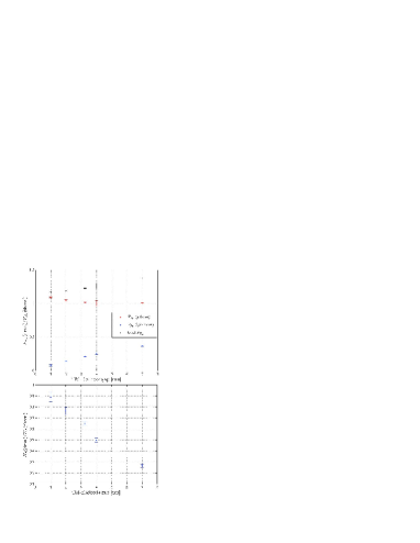
Figure 13: Results of numerical simulations for the radiometer effect, as a function of the gap (in mm) between test mass and electrodes of the position sensor. The top panel shows the ratio of the simulation torque to that calculated from Eqn.3, for the $x$ component of the force acting on the TM $X$ faces (red dots), for the $x$ force acting on the $Y$ and $Z$ TM faces (blue dots) and for the total $x$ force acting on the TM (sum of previous values, shown as green dots). The bottom panel shows the ratio of the simulated torque, around the $z$ (or $y$ axis, to the infinite plate result (Eqn.5), for the $Y$ (or $Z$) face. The average of the magnitudes for the 4 $X-Y$ faces has been reported. While all other calculations are made for equal gaps in all directions, the point at 3.2 mm is calculated with the real gaps of the configuration baselined both for LISA Pathfinder and LISA and shown in Fig.1.

Each time a particle hits a TM face, it completely transfers its momentum to the TM. Upon reemission, it transfers the recoil momentum to the TM and then flies at constant velocity until it reaches another surface. Momenta and angular momenta transferred to the TM are summed bounce by bounce, as well as the flying time between bounces. At the end, the total linear and angular momenta transferred to the TM are divided by the total elapsed time, giving the average force and torque acting on the TM. This calculation has been performed for each momenta component transferred to each TM face. For each geometrical configuration, roughly 10 runs each consisting of roughly $5\times 10^{7}$ bounces were performed. The resulting force and torque values were averaged and the standard deviation calculated to determine the calculation uncertainties.
The results of the calculation are summarized in Fig.13.The GRS design under construction for LISA Pathfinder and currently proposed for LISA, is represented in Fig.13 by the point at 3.2 mm. In Sec. II.1these results are illustrated and discussed.

Appendix B Thermal radiation pressure: numerical simulations

The effective role of thermal radiation pressure has been evaluated in the simplified GRS geometry, with a cubic TM contained and centered inside a rectangular box, by numerical simulations. The eventual modifications to the radiation pressure “transfer function” can be calculated and expressed as the correction factors $\kappa_{RP}$ and $\gamma_{RP}$ introduced in Sec. II.2, for comparison to the simple model discussed there.

For the simulations, the total forces and torques on the TM associated with thermal radiation have been represented as an integral of $T^{4}$ multiplied by an independent vectorial force or torque function, $\overrightarrow{f}(\mathbf{r})$ or $\overrightarrow{n}(\mathbf{r})$, representing the contribution (per K⁴) of thermal photons originating from the sensor surface element $d\mathbf{s}$ at position $\mathbf{r}$ of the EH surfaces $\mathbf{S}$:

$$\overrightarrow{F}_{RP} = \sum_{(\text{EH,TM faces})}\int\overrightarrow{f}(\mathbf{r})T^{4}(\mathbf{r})d\mathbf{s}$$

$$\overrightarrow{N}_{RP} = \sum_{(\text{EH, TM faces})}\int\overrightarrow{n}(\mathbf{r})T^{4}(\mathbf{r})d\mathbf{s}$$

In the infinite plate limit (see Eqn.8), $f_{x}=\mp\frac{2\sigma}{3c}$ for sensor surface elements directly opposite the TM faces on the $X_{+}$ and $X_{-}$ faces (the yellow and orange zones at left in Fig.5), respectively, and zero elsewhere in the sensor. For the torque, $n_{z}=\frac{2\sigma}{3c}\times b(\mathbf{s})$, where the effective armlength $b(\mathbf{s})=\pm y$ for the orange and yellow zones at right in Fig.5 (and, analogously, $\pm x$ for the corresponding zones on the $Y$ faces). The functions $\overrightarrow{f}(\mathbf{r})$ and $\overrightarrow{n}(\mathbf{r})$ depend only on the sensor geometry and reflection properties, and so can be evaluated point-by-point and independently of the sensor temperature distribution.

In the simulations, a chosen number of photons is emitted from a given position of the TM or of the EH surfaces. Photon angle is determined statistically, again assuming a uniform probability density in $\phi$ and $\cos^{2}\left(\theta\right)$. The surface absorption properties were assumed to be independent of wavelength, which allowed for a simple normalization for the number of photons (or effective time of the simulation) and the resulting forces, using the Stefan-Boltzmann law for the radiated power from a surface element of given absorption coefficient $a$, $\left(a\sigma T^{4}\right)$, and the energy - momentum relation for photons, $E=pc$. Each emitted photon is propagated ballistically from the emitting surface, and then either absorbed or reflected statistically, according to the surface absorption properties imposed. In the case of reflection, specular or diffuse (statistical angular reemission) was decided statistically with the imposed percentage of diffuse scattering, $d$. At each collision with the TM, the momentum and moment of the momentum transfer are recorded and then summed at the end of the simulation to determine the total force and torque on the TM.

For the cases studied here, emission from the TM was not calculated, as, in the isothermal TM-approximation reasonable for LISA and our experiments, the TM radiation produces no net recoil. Additionally, for simplicity, the absorption properties were assumed to be uniform and equal for the TM and sensor surfaces. The points of emission for which the simulation was performed were uniformly distributed on the faces of the sensor, using a rectangular grid with $0.5$ mm spacing. Each simulation, typically involving $200$ photons, was repeated, typically $5$ times, for each point inside the sensor, in order to obtain the uncertainties for $\overrightarrow{f}(\mathbf{r})$ and $\overrightarrow{n}(\mathbf{r})$.

Simulations have been performed for several different sensor geometries, including the two studied experimentally in this paper. Additionally, simulations have been performed for several sets of reflection properties: ($i$) absorptivity $a=100\%$ ($ii$) absorptivity = $a=10\%$ and pure diffusive reflection $(d=100\%)$ ($iii$) absorptivity $a=10\%$ and pure specular reflection $(d=0\%)$ ($iv$) absorptivity = $a=5\%$ and pure diffusive reflection $(d=100\%)$ ($v$) absorptivity $a=5\%$ and pure specular reflection $(d=0\%)$.

Finally, in order to obtain the relevant radiometric effect correction factors for the $x$-force and the $z$-torque, $\kappa_{RP}$ and $\gamma_{RP}$, the values of $\overrightarrow{f}(\mathbf{r})$ and $\overrightarrow{n}(\mathbf{r})$ obtained from the simulation must be multiplied by $\left(T(\mathbf{r})\right)^{4}$, with the sensor temperature distribution $T(\mathbf{r})$ chosen to represent a specific experimental thermal perturbation. Results for cases relevant to thermal gradient forces and torques are discussed below.

B.1 Radiation pressure simulation results: induced force

For the study of the radiation pressure force along $x$, we plot first the relevant force function $f_{x}(\mathbf{r})$, normalized by the infinite plate value $\left(2\sigma/3c\right)$, as a function of the emission position $\mathbf{r}$ on the sensor $X$ and $Y$ faces (the $Z$ faces play a role very analogous to that of the $Y$ faces for the $x$ force). These are shown for the LISA Pathfinder sensor design in Fig.14 ($X$ faces - left column, $Y$ faces - right column), together with infinite plates model case. Then, to calculate the relevant factor $\kappa_{RD}$, integration of $f_{x}$ is performed for a temperature distribution with a gradient in the $x$ direction, with each $X$ face at a uniform temperature and a linear temperature gradient across the $Y$ and $Z$ faces. The resulting values for the correction factor $\kappa_{RP}$ are summarized for different sensor geometries and absorptivity characteristics in Table 2. The table also gives a breakdown of the contributions to $\kappa_{RP}$, including not only the contribution expected from the $X$ faces directly opposite the TM ($\kappa_{X(IN)}$), but also those not foreseen by the infinite plate model, from the borders of the $X$ sensor faces ($\kappa_{X(OUT)}$) and from the other sensor faces ($\kappa_{YZ}$).

As visible in Fig.14($2^{nd}$ row, left), where we consider full absorption of emitted photons ($a=100\%$), for emission from near the center of the sensor $X$ faces, $f_{x}/\left(2\sigma/3c\right)\approx 1$, as expected for the infinite plate model ($1^{st}$ row left). Approaching and crossing the edge of the TM, $f_{x}/\left(2\sigma/3c\right)$ decreases smoothly from one towards zero, as a continuously smaller fraction of the emitted photons strike the TM surface. For runs with the smallest gaps (not plotted here), the transition near the edge of the TM becomes sharper, and the infinite plate model becomes more accurate. Additionally, there is a significant contribution of emission from the $Y$ faces to $f_{x}$ Fig.14(right column). The zones near the edges adjacent to the $X_{+}$ and $X_{-}$ faces contribute photons that are predominantly absorbed on the TM near the center of the $Y$ face, and as such exert a shear force along $x$. There is an analogous contribution from the $Z$ face. When integrated with the temperature distribution, this shear force contribution is largely responsible for the increase in the radiation pressure effect ($\kappa_{RP}=1.17$, Table 2). We note that this increase in the case of full absorption is similar to that seen for the radiometric effect, with the shear forces along the $Y$ and $Z$ faces a leading factor in both cases. Also in Table 2, we see that with 200 micron gaps, the simulation confirms the infinite plate model, $\kappa_{RP}=1$ to better than 1%, nearly entirely from the contribution of the $X$ faces opposite the sensor $\kappa_{x(IN)}$.

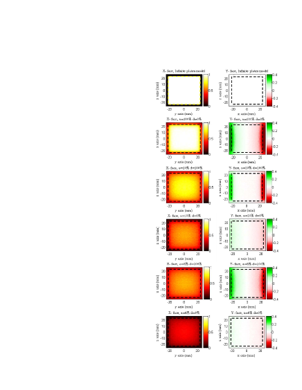
Figure 14: Intensity plots of the $x$ component of the force function $f_{x}(\mathbf{r})$, the force per K⁴ per unit area of emitting sensor surface $K^{4}$, normalized by $\left(2\sigma/3c\right)$, the characteristic value of the infinite model. Results are shown for emitting points on the $X$ (left column) and $Y$ surfaces (right column), with the outline of the TM section a dashed-line 46 mm square in each case. The $1^{st}$ row shows the data for the infinite plates model. Rows 2 to 6 show the different cases of reflection properties: full absorption, $a=100\%$, absorption coefficient $a=10\%$ or $a=5\%$, pure diffusive reflection ($d=100\%$) or purely specular reflection ($d=0\%$). Legends for the intensity values are shown in the colors bars on the right of each plot.

With higher reflectivity, i.e. low $a$ ($3^{rd}$ to $6^{th}$ row, left), the effect of smoothing the $X$ face contribution is more pronounced, as even photons emitted near the center of the $X$ face can migrate off the TM $X$ face and deposit their momentum on other faces, even on the opposite TM $X$ face. The smoothing is more pronounced for specular scattering than diffuse, because in diffuse scattering the effective distance traveled by the photons increases only as the square root of the number of bounces, in a random walk, rather than linearly as for specular reflection. The extreme case of high reflectivity and specular reflection ($a=5\%$ and $d=0\%$, bottom left) represents a progressive homogenization of the radiation pressure, as a photon generated from any point in the sensor winds up imparting momentum on different parts of the TM, effectively washing out also the shear effect (see Fig.14, bottom right). As a value for adsorption around $5\div 10\%$ and specular reflection is the likely case for the gold coated surfaces envisioned for the LISA GRS, a reasonable estimate of the radiation pressure correction for LISA ranges between $\kappa_{RP}=\left(0.32\pm 0.01\right)$ and $\kappa_{RP}=\left(0.63\pm 0.02\right)$ (the errors given are simply the statistical uncertainties of the simulation).

GRS Geometry	(absortivity,	$\kappa_{RP}$	$\kappa_{X(IN)}$	$\kappa_{X(OUT)}$	$\kappa_{YZ}$
(TM , gap)	diffusion)
	(100%,0%)	1.17	0.95	0.05	0.17
	(10%, 100%)	1.01	0.69	0.05	0.28
(46mm3, 4mm)	(10%, 0%)	0.63	0.50	0.02	0.10
	(5%, 100%)	0.75	0.49	0.03	0.23
	(5%, 0%)	0.32	0.26	0.01	0.05
	(100%,0%)	1.12	0.96	0.04	0.12
	(10%, 100%)	1.01	0.78	0.03	0.21
(40mm3, 2mm)	(10%, 0%)	0.75	0.64	0.02	0.10
	(5%, 100%)	0.85	0.62	0.03	0.20
	(5%, 0%)	0.45	0.39	0.01	0.05
	(100%,0%)	0.999	0.986	0.002	0.01
(46mm3, 0.2mm)	(10%, 100%)	0.966	0.937	0.002	0.027
	(10%, 0%)	0.946	0.906	0.002	0.038
	(100%,0%)	100	0.985	0.002	0.013
(40mm3, 0.2mm)	(10%, 100%)	0.963	0.929	0.002	0.031
	(10%, 0%)	0.942	0.896	0.002	0.043

Table 2: The overall correction factor $\kappa_{RP}$ estimated in the case of a linear temperature profile across the sensor along x axis, and the X+ and X- faces at uniform temperature;$\kappa=\left(\kappa_{x_{in}}+\kappa_{x_{out}}+\kappa_{(y+z)}\right)$ and $\kappa_{x_{in}}$, $\kappa_{x_{out}}$ and $\kappa_{(y+z)}$ representing respectively the contributions from the $X$ faces facing the TM, the $X$ faces not facing the TM and the lateral $Y$ and $Z$ faces. The simulations were performed for different GRS geometries (i.e. different gap); the one indicated with (46mm³, 4mm) is the GRS geometry under construction for LISA Pathfinder and currently baselined for LISA. Statistical errors in each estimate of $\kappa_{RP}$ are in the order of $2\div 4\%$.

B.2 Radiation pressure simulation results: induced torques

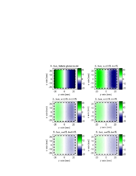
Figure 15: Intensity plot of the torque per unit area $n_{z}(\mathbf{r})$ about the $z$ axis, normalized here by the factor $\left(2\sigma/3c\right)$, for emitting points on the $X$ surface (the $y$ face of the EH shows the exact same profile). the $1^{st}$ plot (top left) shows the infinite plates model case. The various cases of full absorption, $a=100\%$, absorption coefficient $a=10\%$ or $a=5\%$, pure diffusive reflection ($d=100\%$) or purely specular reflection ($d=0\%$) are shown.

In Fig.15 we show the $z$ components $n_{z}(\mathbf{r})$ of the torques per unit area per K⁴ as a function of the position inside the EH and as a function of the GRS surface properties. We still use the normalization factor $\left(2\sigma/3c\right)$: we thus remark that $n_{z}(\mathbf{r})/\left(2\sigma/3c\right)=b(\mathbf{r})$ for the infinite plate approximation (shown in Fig.15 top left), which coincides in the particular case of the $X$ face of the EH under consideration with the $y$ coordinate, and with the $x$ coordinate on the $Y$ face. The different cases of surface reflectivity are here shown (left to right, top to bottom).

As is visible, a reduction similar to that observed for the force is seen for the thermal radiation torque. However, in this case, the effect is much more relevant: the overall attenuation of $N_{z}$ is much more effective, because the attenuation of $f_{z}(\mathbf{r})$ is progressively more effective approaching the edges of the TM. It thus gets reduced exactly where the arm-length $b(\mathbf{r})$ is bigger and the torque per unit area should contribute most to the overall effect. This is clearly visible in the data in Table 3, where we report the estimates of the radiation pressure induce torque correction factors $\gamma_{RP}$, for an ideal linear temperature profile on one of the faces of the IS (with zero temperature modulation on the other faces). We estimate the total torque to be reduced down to $\approx 73\%$ compared to the theoretical estimate in the case of $100\%$ absortivity. In the case of absortivity of the IS surfaces of order $10\%$ or lower, the reduction is then much more relevant, and we estimate the total torque to be suppressed down to a value between $15\%$ for EM4mm and $24\%$ for TN2mm of the theoretical value, in the realistic case of reflectivity $95\%$ ($a=5\%$) and pure specular reflection ($d=0\%$)(see Table 3).

GRS Geometry	(absorptivity,	$\gamma_{tot}$
(TM , gap)	diffusion)
	(100%,0%)	0.73
(46mm3, 4mm)	(10%, 100%)	0.30
	(10%, 0%)	0.27
	(5%, 100%)	0.17
	(5%, 0%)	0.15
	(100%,0%)	0.80
(40mm3, 2mm)	(10%, 100%)	0.42
	(10%, 0%)	0.39
	(5%, 100%)	0.27
	(5%, 0%)	0.24

Table 3: Correction factors $\gamma_{RP}$ for the thermal radiation pressure induced torques. The GRS geometries here reported (46mm³, 4mm and 40mm³, 2mm) correspond to the two GRS prototypes studied with the torsion pendulum (EM4mm and TN2mm respectively). Statistical errors are in the order of $2\div 4\%$.

Appendix C Estimate of temperature patterns and thermal integrals

As mentioned in Sec. III.3, for each measurements cycle we evaluate the component at frequency $\omega$ of the “thermal torque” $\left(\int_{S}T(s)b(s)ds\right)_{(\omega)}$ with the equation

$$\left(\int_{S}T(s)b(s)ds\right)_{\omega} = \sum_{X_{+},X_{-}}\int_{A}(\pm)T(y,z,\omega)ydydz+$$ (18)

$$+ \sum_{Y_{+},Y_{-}}\int_{A}\left(\mp\right)T(x,z,\omega)xdydz.$$

The components $T(s_{1},s_{2},\omega)$ of the temperature at position$(s_{1},s_{2})$, where $s_{1}$ and $s_{2}$ are two coordinates mapping the 4 $X$-$Y$ sensor surfaces, have been estimated by a cubic spatial interpolation of the components $T(s_{1},s_{2},\omega)_{i}$ of the readings $T_{i}(t)$ of the thermometers on the external electrode housing surface at the positions $(s_{1},s_{2})_{i}$, which were measured during assembly. In performing the interpolation, several important approximations were made and are addressed in the next two paragraphs.

Figure 4 shows a cartoon of the two GRS prototypes with the locations of the thermometers (small blue squares). For the EM4mm prototype, six of the eight installed thermometers were used for the interpolation, namely $T1$, $T2$, $T3$, $T4$, $T7$, and $T8$. For TN2mm, four of the five thermometers were used for the interpolation ($T2$, $T3$, $T5$ and $T6$). In this case, the reading of $T5$ was assigned to the temperature at the center of the heater H1E, in order to constrain the local temperature maximum to coincide with the heater location. Additionally, in order to construct the temperature distribution on the TN2mm $X+$ face, which has only a single thermometer, in contrast with the three $X-$ face thermometers, we introduced an artificial thermometer reading, $T_{fake}$ near the heater H2W. The modulation of $T_{fake}$ was assigned to be the value of the interpolated component at the center of the electrode below H2E on the opposing $X-$ face, scaled by the ratio $\frac{T_{2}}{T_{4}}$, in order to account for observed asymmetric heating for the two $X$ faces.

Figure 16 shows an example of a reconstructed temperature profile $T(s_{1},s_{2},\omega)$ across the entire sensor TN2mm. Several assumptions were made in making this estimation, for both sensors. First, the temperature on the inner surface of the sensor is assumed to be equal to that on the corresponding outer surface position, as calculated by the interpolated the outer surface thermometer readings. Additionally, the temperature profile along the $z$ axis (that parallel to the torsion fiber in our experiments) was collapsed to a single value, that of the temperature readings interpolated in the horizontal dimension. The measured temperatures are thus assumed to represent the average temperatures along the sensor $z$ axis at a given value of the horizontal coordinate $x$ (or $y$, depending on the face). These assumptions clearly result in some systematic error in the estimation of the thermal integral, which is discussed next.

The temperature read by a thermometer on the GRS external surface is a good approximation of that measured on corresponding the inner GRS surface position, as long as the thermometer is not too close to an operating heater or to relevant localized thermal interfaces, such as the supporting legs at the four lower corners of the sensor. All the thermometers used in the interpolation are indeed far from these corner supporting legs, and, additionally, they are all placed at least 9 mm from the border of the heaters, a distance equal to the sensor wall thickness, including the electrode. A simplified FEM model has confirmed that the inside-outside temperature difference can indeed be considered negligible in these conditions.

As stated above, the thermometer readings used for the interpolation are assumed to be the average temperature value along $z$. For the $Y$ faces, where there are no heaters, the main effect of the temperature variation along $z$ is expected to be an altitude-dependent offset of the whole profile, with a negligible impact on the thermal integral $\int_{S}T(\mathbf{s})b(\mathbf{s})ds$, where a constant temperature offset integrates to zero. For the $X$ faces, however, the operating heaters produce a more complicated and more rapidly varying temperature pattern. Moreover, the inner surface temperature modulation in correspondence with the operating heater is expected to be relatively uniform across the heater, but higher than that measured by the closest thermometer. A rough estimation of the consequent correction to the temperature pattern on the $X$ faces has been obtained by assuming that the heat flux in the proximity of a cylindrical heater is basically radial and uniform, an approximation supported by a simplified FEM calculation. In this approximation, we estimate that our simple interpolation technique underestimates the thermal integral by roughly $30\%$ for the UTN2mm and $20\%$ for the EM4mm. However, given the approximate nature of the analysis and the experimental difficulty of verifying this model with a tight array of thermometers on the inner sensor surfaces, we choose here not to correct the data for this likely systematic error. Instead, we present the data obtained from the relatively straightforward interpolation and discuss the role of this systematic error in the conclusion of our data analysis.

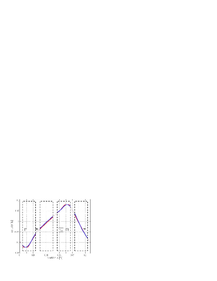
Figure 16: An example of the temperature profile across the entire sensor TN2mm. Blue line: derived from cubic interpolation of the thermometer readings. Red line: based on a constant temperature across the electrodes with operating heaters and a linear interpolation of the thermometer readings across the rest of the sensor. A single temperature is assigned for all values of $z$ at each given value the horizontal coordinate $s$ ($x$ or $y$, depending on the face).

In order to address the dependence of the thermal integral calculation on the method of spatial interpolation, we compare the results of two different methods, both of which reasonably reproduce the expected relatively uniform temperature profile of the “hot” electrodes coinciding with the locations of active heaters (see Fig.16). The first calculation assumes a perfectly constant temperature across the “hot” electrodes and a linear interpolation for the rest of the temperature profile. These results are compared with that obtained with the cubic polynomial interpolation. Thanks to the higher number of thermometers, for the EM4mm prototype the difference was negligible, while for the TN2mm model the first method gave a value $20\%$ larger than the second.

Considering the approximate analysis of the different sources of uncertainty in the thermal integral, we conservatively assume the overall uncertainty to be the linear sum of the above estimated errors. This yields an uncertainty of roughly $50\%$ for the TN2mm prototype and roughly $20\%$ for EM4mm. Given that the same heating pattern is repeated in all measurements presented for each of the two sensors, this uncertainty in the thermal integral estimation can be thought of as a single scale factor for the each of the two sensor data sets, rather than an uncertainty acting incoherently on different data points in the same sensor. Unless otherwise specified, the error bars of the torque data normalized by means of the ”thermal integral”, namely $N^{*}$ represents just the statistical error of the torque measurement $N$. The role of this scale factor will be discussed with the conclusion of our data analysis in Sec. IV.

- (1) P. Bender et al, LISA ESA-SCI(2000)11, 2000.
- (2) http://einstein.stanford.edu/, http://www.gravityprobeb.com
- (3) STEP Satellite Test of the Equivalence Principle, Report on the Phase A Study, ESA/NASA-SCI(93)4, 1993.
- (4) www.cnes.fr/activities/connaissance/ physique/microsatellite/
- Dolesi et al. (2003) R. Dolesi et al., Class. Quant. Grav. 20, S99 (2003).
- Stebbins et al. (2003) R.T. Stebbins et al., Classical and Quantunm Gravity 21, S653 (2004).
- Schumaker et al. (2003) B.L. Schumaker, Classical and Quantum Gravity 20, S239 (2003).
- Weber et al. (2002b) W. J. Weber et al., SPIE Proc. 4856, 31 (2002b).
- Hueller et al. (2005) M. Hueller ,et al., Classical and Quantum Gravity 22, S521 (2005).
- (10) S. Vitale et al., Nuclear Physics B, v.110, p.209, 2002
- Anza et al. (2005) S. Anza et al., Class. Quant. Grav. 22, S125 (2005).
- Hueller et al. (2002) M. Hueller et al., Class. Quant. Grav. 19, 1757 (2002).
- Carbone et al. (2007) L. Carbone et al., Phys. Rev. D 75, 042001 (2007).
- Carbone et al. (2003) L. Carbone et al., Phys. Rev. Lett. 91, 151101 (2003).
- Carbone et al. (2003) L. Carbone et al., Class. Quant. Grav. 21, S611 (2004).
- (16) L.Carbone, Ground based investigation of force noise sources for LISA, PhD Thesis, University of Trento, Feb. 2005
- Carbone et al. (2005) L. Carbone et al., Class. Quant. Grav. 22, S509 (2005).
- (18) S. Schlamminger et al, Proceedings of the 6th International LISA Symposium, AIP Conf. Proc.,873, 151-157 (2006).
- Nobili et al. (2001) A.M. Nobili et al., Phys. Rev. D 63, 101101(R) (2001).
- Nobili et al. (2002) A.M. Nobili et al., New Astronomy 7, 521 (2002).
- (21) S. E. Pollack et al., Proceedings of the 6th international LISA Symposium, AIP Conf. Proc.,873, 158-164 (2006).
- (22) P.L. Bender, Proceedings of the 6th international LISA Symposium, AIP Conf. Proc.,873, 143-150 (2006).
- (23) S.M. Merkowitz, Proceedings of the 6th international LISA Symposium, AIP Conf. Proc.,873, 133-142 (2006).
- (24) A. Roth , Vacuum Technology, North Holland (1982)
- Wu Y. et al. (2002) Y. Wu, J. Vac. Sci. Technol. 9, 1248 (1972).
- Wu (2002) Y. Wu, J. of Chem. Phys. 48, 889 (1968).
- (27) Thermal Radiative Properties: metallic elements and alloys,Thermophysiscal prop. of Matter, the TPRC Data Series 7, 244-245.
- (28) S. Vitale, Unitn-Int-1-2003, 2003.
- (29) A. Rüdiger, Residual gas effects in space-borne position sensors, MPI für Gravitationsphysik, AEI Hannover, unpublished, (2002)
- (30) J.F.O’Hanlon, A User Guide to Vacuum Technology, Wiley-Interscience Publication(1989)
- (31) W.Steckelmacher and M.W.Lucas, J.Phys.D: Appl.Phys.,16, 1453-1460 (1983).
- (32) L. Carbone et al, Proceedings of the 6th international LISA Symposium, AIP Conf. Proc.,873, 561-565 (2006).