Quadratic optimal functional quantization of stochastic processes and numerical applications
Abstract
In this paper, we present an overview of the recent developments of functional quantization of stochastic processes, with an emphasis on the quadratic case. Functional quantization is a way to approximate a process, viewed as a Hilbert-valued random variable, using a nearest neighbour projection on a finite codebook. A special emphasis is made on the computational aspects and the numerical applications, in particular the pricing of some path-dependent European options.
Index
1 Introduction
Functional quantization is a way to discretize the path space of a stochastic process. It has been extensively investigated since the early 2000’s by several authors (see among others [29], [31], [12], [9], [30], etc). It first appeared as a natural extension of the Optimal Vector Quantization theory of (finite-dimensional) random vectors which finds its origin in the early 1950’s for signal processing (see [15] or [17]).
Let us consider a Hilbertian setting. One considers a random vector defined on a probability space taking its values in a separable Hilbert space (equipped with its natural Borel -algebra) and satisfying . When is an Euclidean space (), one speaks about Vector Quantization. When is an infinite dimensional space like (endowed with the usual Hilbertian norm ) one speaks of functional quantization (denoted from now on). A (bi-measurable) stochastic process defined on satisfying - can always be seen, once possibly modified on a -negligible set, as an -valued random variable. Although we will focus on the Hilbertian framework, other choices are possible for , in particular some more general Banach settings like or spaces.
This paper is organized as follows: in Sections 2 we introduce quadratic quantization in a Hilbertian setting. In Section 3, we focus on optimal quantization, including some extensions to non quadratic quantization. Section 4 is devoted to some quantized cubature formulae. Section 5 provides some classical background on the quantization rate in finite dimension. Section 7 deals with functional quantizations of Gaussian processes, like the Brownian motion, with a special emphasis on the numerical aspects. We present here what is, to our guess, the first large scale numerical optimization of the quadratic quantization of the Brownian motion. We compare it to the optimal product quantization, formerly investigated in [44]. In section, we propose a constructive approach to the functional quantization of scalar or multidimensional diffusions (in the Stratanovich sense). In Section 9, we show how to use functional quantization to price path-dependent options like Asian options (in a heston stochastic volatility model). We conclude by some recent results showing how to derive universal (often optimal) functional quantization rate from time regularity of a process in Section 10 and by a few clues in Section 11 about the specific methods that produce some lower bounds (this important subject as many others like the connections with small deviation theory is not treated in this numerically oriented overview. As concerns statistical applications of functional quantization we refer to [53, 54].
Notations. means and ; means .
If (Hilbert space), then .
denotes the integral part of the real .
2 What is quadratic functional quantization?
Let denote a separable Hilbert space. Let a random vector ( is endowed with its Borel -algebra) such that . An -quantizer (or -codebook) is defined as a subset
with card. In numerical applications, is also called grid. Then, one can quantize (or simply discretize) by where is a Borel function. It is straightforward that
so that the best pointwise approximation of is provided by considering for a nearest neighbour projection on , denoted . Such a projection is in one-to-one correspondence with the Voronoi partitions (or diagrams) of induced by the Borel partitions of satisfying
where denotes the closure of in (this heavily uses the Hilbert structure). Then
is a nearest neighbour projection on . These projections only differ on the boundaries of the Voronoi cells , . All Voronoi partitions have the same boundary contained in the union of the median hyperplanes defined by the pairs , . Figure 1 represents the Voronoi diagram defined by a (random) -tuple in .

|
Then, one defines a Voronoi -quantization of by setting for every ,
One clearly has, still for every , that
The mean (quadratic) quantization error is then defined by
| (1) |
The distribution of as a random vector is given by the -tuple of the Voronoi cells. This distribution clearly depends on the choice of the Voronoi partition as emphasized by the following elementary situation: if , the distribution of is given by , and since . However, if weights no hyperplane, the distribution of depends only on .
As concerns terminology, Vector Quantization is concerned with the finite dimensional case – when – and is a rather old story, going back to the early 1950’s when it was designed in the field of signal processing and then mainly developed in the community of Information Theory. The term functional quantization, probably introduced in [41, 29], deals with the infinite dimensional case including the more general Banach-valued setting. The term “functional” comes from the fact that a typical infinite dimensional Hilbert space is the function space . Then, any (bi-measurable) process can be seen as a random vector taking values in the set of Borel functions on . Furthermore, if and only if since
3 Optimal (quadratic) quantization
At this stage we are lead to wonder whether it is possible to design some optimally fitted grids to a given distribution which induce the lowest possible mean quantization error among all grids of size at most . This amounts to the following optimization problem
| (2) |
 |
 |
It is convenient at this stage to make a correspondence between quantizers of size at most and -tuples of : to any -tuple corresponds a quantizer (of size at most ). One introduces the quadratic distortion, denoted , defined on as a (symmetric) function by
Note that, combining (1) and the definition of the distortion, shows that
so that,
The following proposition shows the existence of an optimal -tuple such that . The corresponding optimal quantizer at level is denoted . In finite dimension we refer to [49] (1982) and in infinite dimension to [7] (1988) and [48] (1990); one may also see [39], [17] and [29]. For recent developments on existence and pathwise regularity of optimal quantizer see [20].
Proposition 1
The function is lower semi-continuous for the product weak topology on .
The function reaches a minimum at a -tuple (so that is an optimal quantizer at level ).
– If , the quantizer has full size ( ) and .
– If , .
Furthermore .
Any optimal (Voronoi) quantization at level , satisfies
| (3) |
where denotes the -algebra generated by .
Any optimal (quadratic) quantization at level is a best least square ( ) approximation of among all -valued random variables taking at most values:
Proof (sketch of): The claim follows from the l.s.c. of for the weak topology and Fatou’s Lemma.
One proceeds by induction on . If , the optimal -quantizer is and .
Assume now that an optimal quantizer does exist at level .
– If , then the -tuple (among other possibilities) is also optimal at level and .
– Otherwise, , hence has pairwise distinct components and there exists .
Then, with obvious notations,
Then, the set is non empty, weakly closed since is l.s.c.. Furthermore, it is bounded in . Otherwise there would exist a sequence such that as . Then, by Fatou’s Lemma, one checks that
Consequently is weakly compact and the minimum of on is clearly its minimum over the whole space . In particular
If , set (as sets) so that t which implies .
To establish that goes to , one considers an everywhere dense sequence in the separable space . Then, goes to as for every . Furthermore, . One concludes by the Lebesgue dominated convergence Theorem that goes to as .
and Temporarily set for convenience. Let be a random vector taking at most values. Set . Since is a Voronoi quantization of induced by ,
so that
On the other hand, the optimality of implies
Consequently
The inequality holds as an equality since takes at most values. Furthermore, considering random vectors of the form (which take at most as many values as the size of ) shows, going back to the very definition of conditional expectation, that -
Item introduces a very important notion in (quadratic) quantization.
Definition 1
A quantizer is stationary (or self-consistent) if (there is a nearest neighbour projection such that satisfying)
| (4) |
Note in particular that any stationary quantization satisfies .
As shown by Proposition 1 any quadratic optimal quantizer at level is stationary. Usually, at least when , there are other stationary quantizers: indeed, the distortion function is -differentiable at -quantizers with pairwise distinct components and
hence, any critical points of is a stationary quantizer.
Remarks and comments. In fact (see Theorem 4.2, p. 38, [17]), the Voronoi partitions of always have a -negligible boundary so that (4) holds for any Voronoi diagram induced by .
The problem of the uniqueness of optimal quantizer (viewed as a set) is not mentioned in the above proposition. In higher dimension, this essentially never occurs. In one dimension, uniqueness of the optimal -quantizer was first established in [14] with strictly -concave density function. This was successively extended in [23] and [55] and lead to the following criterion (for more general “loss” functions than the square function):
If the distribution of is absolutely continuous with a -concave density function, then, for every , there exists only one stationary quantizer of size , which turns out to be the optimal quantizer at level .
More recently, a more geometric approach to uniqueness based on the Mountain Pass Lemma first developed in [26] and then generalized in [6]) provided a slight extension of the above criterion (in terms of loss functions).
This -concavity assumption is satisfied by many families of probability distributions like the uniform distribution on compact intervals, the normal distributions, the gamma distributions. There are examples of distributions with a non -concave density function having a unique optimal quantizer for every (see the Pareto distribution in [16]). On the other hand simple examples of scalar distributions having multiple optimal quantizers at a given level can be found in [17].
A stationary quantizer can be sub-optimal. This will be emphasized in Section 7 for the Brownian motion (but it is also true for finite dimensional Gaussian random vectors) where some families of sub-optimal quantizers – the product quantizers designed from the Karhunen-Lov̀e basis – are stationary quantizers.
For the uniform distribution over an interval , there is a closed form for the optimal quantizer at level given by . This -quantizer is optimal not only in the quadratic case but also for any -quantization (see a definition further on). In general there is no such closed form, either in or higher dimension. However, in [16] some semi-closed forms are obtained for several families of (scalar) distributions including the exponential and the Pareto distributions: all the optimal quantizers can be expressed using a single underlying sequence defined by an induction .
In one dimension, as soon as the optimal quantizer at level is unique (as a set or as an -tuple with increasing components), it is generally possible to compute it as the solution of the stationarity equation (3) either by a zero search (Newton-Raphson gradient descent) or a fixed point (like the specific Lloyd I procedure, see [24]) procedure.
In higher dimension, deterministic optimization methods become intractable and one uses stochastic procedures to compute optimal quantizers. The main topic of this paper being functional quantization, we postponed the short overview on these aspects to Section 7, devoted to the optimal quantization of the Brownian motion. But it is to be noticed that all efficient optimization methods rely on the so-called splitting method which increases progressively the quantization level . This method is directly inspired by the induction developed in the proof of claim of Proposition 1 since one designs the starting value of the optimization procedure at size by “merging” the optimized -quantizer obtained at level with one further point of , usually randomly sampled with respect to an appropriate distribution (see [43] for a discussion).
As concerns functional quantization, , there is a close connection between the regularity of optimal (or even stationary) quantizers and that of form into . Furthermore, as concerns optimal quantizers of Gaussian processes, one shows (see [29]) that they belong to the reproducing space of their covariance operator, to the Cameron-Martin space when . Other properties of optimal quantization of Gaussian processes are established in [29].
Extensions to the -quantization of random variables. In this paper, we focus on the purely quadratic framework ( and -norms), essentially because it is a natural (and somewhat easier) framework for the computation of optimized grids for the Brownian motion and for some first applications (like the pricing of path-dependent options, see section 9). But a more general and natural framework is to consider the functional quantization of random vectors taking values in a separable Banach space . Let , such that for some (the case can also be taken in consideration).
The -level -quantization problem for reads
The main examples for are the non-Euclidean norms on , the functional spaces , , equipped with its usual norm, , etc. As concerns, the existence of an optimal quantizer, it holds true for reflexive Banach spaces (see Pärna (90)) and , but otherwise it may fail even when (see [20]). In finite dimension, the Euclidean feature is not crucial (see [17]). In the functional setting, many results originally obtained in a Hilbert setting have been extended to the Banach setting either for existence or regularity results (see [20]) or for rates see [10], [12], [30], [33].
4 Cubature formulae: conditional expectation and numerical integration
Let be a continuous functional (with respect to the norm ) and let be an -quantizer. It is natural to approximate by . This quantity is simply the finite weighted sum
Numerical computation of is possible as soon as can be computed at any and the distribution of is known. The induced quantization error is used to control the error (see below). These quantities related to the quantizer are also called companion parameters.
Likewise, one can consider a priori the -measurable random variable as a good approximation of the conditional expectation .
4.1 Lipschitz functionals
Assume that the functional is Lipschitz continuous on . Then
so that, for every real exponent ,
(where we applied conditional Jensen inequality to the convex function ). In particular, using that , one derives (with ) that
Finally, using the monotony of the -norms as a function of yields
| (5) |
In fact, considering the Lipschitz functional , shows that
| (6) |
The Lipschitz functionals making up a characterizing family for the weak convergence of probability measures on , one derives that, for any sequence of -quantizers satisfying as ,
where denotes the weak convergence of probability measures on .
4.2 Differentiable functionals with Lipschitz differentials
Assume now that is differentiable on , with a Lipschitz continuous differential , and that the quantizer is stationary (see Equation (4)).
A Taylor expansion yields
Taking conditional expectation given yields
Now, using that the random variable is -measurable, one has
so that
Then, for every real exponent ,
In particular, when , one derives like in the former setting
| (7) |
In fact, the above inequality holds provided is with Lipschitz differential on every Voronoi cell . A similar characterization to (6) based on these functionals could be established.
4.3 Quantized approximation of
Let and be two -valued random vector defined on the same probability space and be a Borel functional. The natural idea is to approximate by the quantized conditional expectation where and are quantizations of and respectively.
Let be a (Borel) version of the conditional expectation satisfying
Usually, no closed form is available for the function but some regularity property can be established, especially in a (Feller) Markovian framework. Thus assume that both and are Lipschitz continuous with Lipschitz coefficients and . Then
Hence, using that is -measurable and that conditional expectation is an -contraction,
The last inequality follows form the definition of conditional expectation given as the best quadratic approximation among -measurable random variables. On the other hand, still using that is an -contraction and this time that is Lipschitz continuous yields
Finally,
In the non-quadratic case the above inequality remains valid provided is replaced by .
5 Vector quantization rate ()
The fact that is a non-increasing sequence that goes to as goes to is a rather simple result established in Proposition 1. Its rate of convergence to is a much more challenging problem. An answer is provided by the so-called Zador Theorem stated below.
This theorem was first stated and established for distributions with compact supports by Zador (see [57, 58]). Then a first extension to general probability distributions on is developed in [5]. The first mathematically rigorous proof can be found in [17], and relies on a random quantization argument (Pierce Lemma).
Theorem 5.1
Sharp rate. Let and for some . Let be the canonical decomposition of the distribution of ( and the Lebesgue measure are singular). Then (if ),
| (8) |
where .
Non asymptotic upper bound (see [33]). Let . There exists such that, for every -valued random vector ,
Remarks. The real constant clearly corresponds to the case of the uniform distribution over the unit hypercube for which the slightly more precise statement holds
The proof is based on a self-similarity argument. The value of depends on the reference norm on . When , elementary computations show that . When , with the canonical Euclidean norm, one shows (see [37] for a proof, see also [17]) that . Its exact value is unknown for but, still for the canonical Euclidean norm, one has (see [17]) using some random quantization arguments,
When the distribution of is purely singular. The rate (8) still holds in the sense that . Consequently, this is not the right asymptotics. The quantization problem for singular measures (like uniform distribution on fractal compact sets) has been extensively investigated by several authors, leading to the definition of a quantization dimension in connection with the rate of convergence of the quantization error on these sets. For more details we refer to [17, 18] and the references therein.
A more naive way to quantize the uniform distribution on the unit hypercube is to proceed by product quantization by quantizing the marginals of the uniform distribution. If , , one easily proves that the best quadratic product quantizer (for the canonical Euclidean norm on ) is the “midpoint square grid”
which induces a quadratic quantization error equal to
Consequently, product quantizers are still rate optimal in every dimension . Moreover, note that the ratio of these two rates remains bounded as .
6 Optimal quantization and
The principle of Quasi-Monte Carlo method () is to approximate the integral of a function with respect to the uniform distribution on , ( denotes the Lebesgue measure on ), by the uniformly weighted sum
of values of at the points of a so-called low discrepancy -tuple (or set). This -tuple can the first terms of an infinite sequence.
If has finite variations denoted – either in the measure sense (see [4, 47]) or in the Hardy and Krause sense (see [38] p.19) – the Koksma-Hlawka inequality provides an upper bound for the integration error induced by this method, namely
where
(with , ). The error modulus denotes the discrepancy at the origin of the -tuple . For every , there exists -valued -tuples such that
| (9) |
where is a real constant only depending on . This result can be proved using the so-called Hammersely procedure (see [38], p.31). When is made of the first terms of a -valued sequence , then the above upper bound has be replaced by (). Such a sequence is said to be a sequence with low discrepancy (see [38] an the references therein for a comprehensive theoretical overview, but also [4, 47] for examples supported by numerical tests). When one only has as , the sequence is said to be uniformly distributed in .
It is widely shared by specialists that these rates are (in some sense) optimal although this remains a conjecture except when . To be precise what is known and what is conjectured is the following:
– Any -valued -tuple satisfies where if (see [52] and also [38] and the references therein), and is a real constant only depending on ; the conjecture is that .
– Any -valued sequence satisfies for infinitely many , where if and and is a real constant only depending on ; the conjecture is that . This follows from the result for -tuple by the Hammersley procedure (see [4]).
Furthermore, as concerns the use of Koksma-Hlawka inequality as an error bound for numerical integration, the different notions of finite variation (which are closely connected) all become more and more restrictive – and subsequently less and less “natural” as a regularity property of functions – when the dimension increases. Thus the Lipschitz continuous function defined by has infinite variation on .
When applying Quasi-Monte Carlo approximation of integrals with “standard” continuous functions on , the best known error bound, due to Proinov, is given by the following theorem.
Theorem 6.1
(Proinov [50]) Assume is equipped with the -norm . Let . For every continuous function ,
where , , is the uniform continuity modulus of (with respect to the -norm) and is a universal constant only depending on .
If , and if , .
Remark. Note that if is Lipschitz continuous, then where denotes the Lipschitz coefficient of (with respect to the -norm).
First, this result emphasizes that low discrepancy sequences or sets do suffer from the curse of dimensionality when a approximation is implemented on functions having a “natural” regularity like Lipschitz continuity.
One also derives from this theorem an inequality between -quantization error of the uniform distribution and the discrepancy at the origin of a -tuple , namely
since the function is clearly -Lipschitz continuous with Lipschitz coefficient . The inequality also follows from the characterization established in (6) (which is clearly still true for non Euclidean norms). Then one may derive some bounds for Euclidean norms (and in fact any norms) on (probably not sharp in terms of constant) since all the norms are strongly equivalent. However the bounds for optimal quantization error derived from Zador’s Theorem ( and those for low discrepancy sets (see (9)) suggest that overall, optimal quantization provides lower error bounds for numerical integration of Lipschitz functions than low discrepancy sets, at least for for generic values of . (However, standard computations show that for midpoint square grids (with points) both quantization errors and discrepancy behave like ).
7 Optimal quadratic functional quantization of Gaussian processes
Optimal quadratic functional quantization of Gaussian processes is closely related to their so-called Karhunen-Loève expansion which can be seen in some sense as some infinite dimensional Principal Component Analysis () of a (Gaussian) process. Before stating a general result for Gaussian processes, we start by the standard Brownian motion: it is the most important example in view of (numerical) applications and for this process, everything can be made explicit.
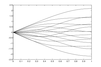
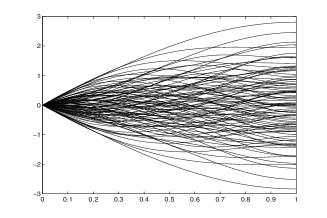
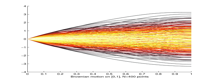
7.1 Brownian motion
One considers the Hilbert space , , . The covariance operator of the Brownian motion is defined on by
It is a symmetric positive trace class operator which can be diagonalized in the so-called Karhunen-Loève (-) orthonormal basis of , with eigenvalues , given by
This classical result can be established as a simple exercise by solving the functional equation . In particular, one can expand itself on this basis so that
Now, the orthonormality of the (-) basis implies, using Fubini’s Theroem,
where denotes the Kronecker symbol. Hence the Gaussian sequence is pairwise non-correlated which implies that these random variables are independent. The above identity also implies that . Finally this shows that
| (10) |
where , , is an i.i.d. sequence of -distributed random variables. Furthermore, this - expansion converges in a much stronger sense since - and
(see [32]). Similar results (with various rates) hold true for a wide class of Gaussian processes expanded on “admissible” basis (see [34]).
Theorem 7.1
For every , with . Furthermore and are independent.
as .
Remark. The fact, confirmed by numerical experiments (see Section 7.3 Figure 6), that holds as a conjecture.
Denoting the orthogonal projection on , one derives from that (optimal quantization at level ) and
where .
7.2 Centered Gaussian processes
The above Theorem 7.1 devoted to the standard Brownian motion is a particular case of a more general theorem which holds for a wide class of Gaussian processes
Theorem 7.2
([29] (2002) and [30] (2004)) Let be a Gaussian process with - eigensystem (with is non-increasing). Let , , be a sequence of quadratic optimal -quantizers for . Assume
and .
.
Remarks. The above result admits an extension to the case as with regularly varying, index (see [30]). In [29], upper or lower bounds are also established when
The sharp asymptotics holds as a conjecture.
Applications to classical (centered) Gaussian processes.
Brownian bridge: , and , , so that .
Fractional Brownian motion with Hurst constant
where and denotes the Gamma function at .
Some further explicit sharp rates can be derived from the above theorem for other classes of Gaussian stochastic processes (see [30], 2004) like the fractional Ornstein-Uhlenbeck processes, the Gaussian diffusions, a wide class Gaussian stationary processes (the quantization rate is derived from the high frequency asymptotics of its spectral density, assumed to be square integrable on the real line), for the -folded integrated Brownian motion, the fractional Brownian sheet, etc.
Of course some upper bounds can be derived for some even wider classes of processes, based on the above first remark (see [29], 2002).
Extensions to When the processes have some self-similarity properties, it is possible to obtain some sharp rates in the non purely quadratic case: this has been done for fractional Brownian motion in [12] using some quite different techniques in which self-similarity properties plays there a crucial role. It leads to the following sharp rates, for and
7.3 Numerical optimization of quadratic functional quantization
Thanks to the scaling property of Brownian motion, one may focus on the normalized case . The numerical approach to optimal quantization of the Brownian motion is essentially based on Theorem 7.1 and the remark that follows: indeed these results show that quadratic optimal functional quantization of a centered Gaussian process reduces to a finite dimensional optimal quantization problem for a Gaussian distribution with a diagonal covariance structure. Namely the optimization problem at level reads
Moreover, if denotes an optimal -quantizer of , then, the optimal -quantizer of reads with
| (11) |
The good news is that is in fact a finite dimensional quantization optimization problem for each . The bad news is that the problem is somewhat ill conditioned since the decrease of the eigenvalues of is very steep for small values of : , . This is probably one reason for which former attempts to produce good quantization of the Brownian motion first focused on other kinds of quantizers like scalar product quantizers (see [44] and Section 7.4 below) or -dimensional block product quantizations (see [56] and [35]).
Optimization of the (quadratic) quantization of -valued random vector has been extensively investigated since the early 1950’s, first in -dimension, then in higher dimension when the cost of numerical Monte Carlo simulation was drastically cut down (see [15]). Recent application of optimal vector quantization to numerics turned out to be much more demanding in terms of accuracy. In that direction, one may cite [43], [36] (mainly focused on numerical optimization of the quadratic quantization of normal distributions). To apply the methods developed in these papers, it is more convenient to rewrite our optimization problem with respect to the standard -dimensional distribution by simply considering the Euclidean norm derived from the covariance matrix
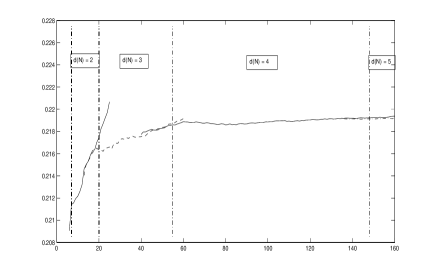
The main point is of course that the dimension is unknown. However (see Figure 6), one clearly verifies on small values of that the conjecture () is most likely true. Then for higher values of one relies on it to shift from one dimension to another following the rule , .
A toolbox for quantization optimization: a short overview
Here is a short overview of stochastic optimization methods to compute optimal or at least locally optimal quantizers in finite dimension. For more details we refer to [43] and the references therein. Let .
Competitive Learning Vector Quantization (). This procedure is a recursive stochastic approximation gradient descent based on the integral representation of the gradient (temporarily coming back to -tuple notation) of the distortion as the expectation of a local gradient
so that, starting from , one sets
where is a real constant to be tuned. As set, this looks quite formal but the operating procedure consists of two phases at each iteration:
Competitive Phase: Search of the nearest neighbor of among the components of , (using a “winning convention” in case of conflict on the boundary of the Voronoi cells).
Cooperative Phase: One moves the winning component toward using a dilatation .
This procedure is useful for small or medium values of . For an extensive study of this procedure, which turns out to be singular in the world of recursive stochastic approximation algorithms, we refer to [40]. For general background on stochastic approximation, we refer to [25, 3].
The randomized “Lloyd I procedure”. This is the randomization of the stationarity based fixed point procedure since any optimal quantizer satisfies (4):
At every iteration the conditional expectation is computed using a Monte Carlo simulation. For more details about practical aspects of Lloyd I procedure we refer to [43]. In [36], an approach based on genetic evolutionary algorithms is developed.
For both procedures, one may substitute a sequence of quasi-random numbers to the usual pseudo-random sequence. This often speeds up the rate of convergence of the method, although this can only be proved (see [27]) for a very specific class of stochastic algorithm (to which does not belong).
The most important step to preserve the accuracy of the quantization as (and ) increase is to use the so-called splitting method which finds its origin in the proof of the existence of an optimal -quantizer: once the optimization of a quantization grid of size is achieved, one specifies the starting grid for the size or more generally , , by merging the optimized grid of size resulting from the former procedure with points sampled independently from the normal distribution with probability density proportional to where denotes the p.d.f. of . This rather unexpected choice is motivated by the fact that this distribution provides the lowest in average random quantization error (see [6]).
As a result, to be downloaded on the website [45] devoted to quantization:
www.quantize.maths-fi.com
Optimized stationary codebooks for : in practice, the -quantizers of the distribution , up to ( runs from up to ).
Companion parameters:
– distribution of : .
– The quadratic quantization error: .
 |
 |
 |
 |
 |
 |
7.4 An alternative: product functional quantization
Scalar Product functional quantization is a quantization method which produces rate optimal sub-optimal quantizers. They were used in [29] to provide exact rate (although not sharp) for a very large class of processes. The first attempts to use functional quantization for numerical computation with the Brownian motion was achieved with these quantizers (see [44]). We will see further on their assets. What follows is presented for the Brownian motion but would work for a large class of centered Gaussian processes.
Let us consider again the expansion of in its - basis :
where is an i.i.d. sequence -distributed random variables (keep in mind this convergence also holds uniformly in ). The idea is simply to quantize these (normalized) random coordinates : for every , one considers an optimal -quantization of , denoted (). For , set and (which is the optimal -quantization). The integer is called the length of the product quantization. Then, one sets
Such a quantizer takes values.
If one denotes by the (unique) optimal quadratic -quantizer of the -distribution, the underlying quantizer of the above quantization can be expressed as follows (if one introduces the appropriate multi-indexation): for every multi-index , set
Then the product quantization can be rewritten as
where the Voronoi cell of is given by
with , , .
Quantization rate by product quantizers
It is clear that the optimal product quantizer is the solution to the optimal integral bit allocation
| (12) |
Expanding yields
| (13) | |||||
| (14) |
Theorem 7.3
(see [29]) For every , there exists an optimal scalar product quantizer of size at most (or at level ), denoted , of the Brownian motion defined as the solution to the minimization problem (12). Furthermore these optimal product quantizers make up a rate optimal sequence: there exists a real constant such that
Proof (sketch of). By scaling one may assume without loss of generality that . Combining (13) and Zador’s Theorem shows
with . Setting and , , yields the announced upper-bound.
Remarks. One can show that the length of the optimal quadratic product quantizer satisfies
The most striking fact is that very few ingredients are necessary to make the proof work as far as the quantization rate is concerned. We only need the basis of on which is expanded to be orthonormal or the random coordinates to be orthogonal in . This robustness of the proof has been used to obtain some upper bounds for very wide classes of Gaussian processes by considering alternative orthonormal basis of like the Haar basis for processes having self-similarity properties (see [29]), or trigonometric basis for stationary processes (see [29]). More recently, combined with the non asymptotic Zador’s Theorem, it was used to provide some connections between mean regularity of stochastic processes and quantization rate (see Section 10 and [33]).
Block quantizers combined with large deviations estimates were used to provide the sharp rate obtained in Theorem 7.1 in [30].
-dimensional block quantization is also possible, possibly with varying block size, providing a constructive approach to sharp rate, see [56] and [35].
A similar approach can also provide some -rates for product quantization with respect to the -norm over , see [32].
How to use product quantizers for numerical computations ?
For numerics one can assume by a scaling argument that . To use product quantizers for numerics we need to have access to the quantizers (or grid) at a given level , their weights (and the quantization error). All these quantities are available with product quantizers. In fact the first attempts to use functional quantization for numerics (path dependent option pricing) were carried out with product quantizers (see [44]).
The optimal product quantizers (denoted ) at level are explicit, given the optimal quantizers of the scalar normal distribution . In fact the optimal allocation of the size of each marginal has been already achieved up to very high values of . Some typical optimal allocation (and the resulting quadratic quantization error) are reported in the table below.
| Quant. Error | Opti. Alloc. | ||
|---|---|---|---|
| 1 | 1 | 0.7071 | 1 |
| 10 | 10 | 0.3138 | 5-2 |
| 100 | 96 | 0.2264 | 12-4-2 |
| 1 000 | 966 | 0.1881 | 23-7-3-2 |
| 10 000 | 9 984 | 0.1626 | 26-8-4-3-2-2 |
| 100 000 | 97 920 | 0.1461 | 34 – 10 – 6 – 4 – 3 – 2 – 2 |
The weights are explicit too: the normalized coordinates of in its - basis are independent, consequently
Equation (14) shows that the (squared) quantization error of a product quantizer can be straightforwardly computed as soon as one knows the eigenvalues and the (squared) quantization error of the normal distributions for the ’s.
The optimal allocations up to can be downloaded on the website [45] as well as the necessary -dimensional optimal quantizers (including the weights and the quantization error) of the scalar normal distribution (up to a size of which quite enough for this purpose).
For numerical purpose we are also interested in the stationarity property since such quantizers produce lower (weak) errors in cubature formulas.
Proposition 2
(see [44]) The product quantizers obtained from the - basis are stationary quantizers (although sub-optimal).
Proof. Firstly, note that
so that . Consequently
Remarks. This result is no longer true for product quantizers based on other orthonormal basis.
This shows the existence of non optimal stationary quantizers.
 |
 |

7.5 Optimal product quadratic functional quantization ()
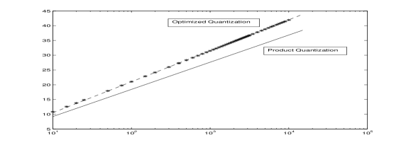
(Numerical) Optimized Quantization: By scaling, we can assume without loss of generality that . We carried out a huge optimization task in order to produce some optimized quantization grids for the Brownian motion by solving numerically for up to .
This value (see Figure 9(left)) is significantly greater than the theoretical (asymptotic) bound given by Theorem 7.1 which is
Our guess, supported by our numerical experiments, is that in fact is possibly not monotonous but unimodal.
Optimal Product quantization: as displayed on Figure 9(right), one has approximately
Optimal -dimensional block product quantization: let us briefly mention this approach developed in [56] in which product quantization is achieved by quantizing some marginal blocks of size , or . By this approach, the corresponding constant is approximately , roughly in between scalar product quantization and optimized numeric quantization.
The conclusion, confirmed by our numerical experiments on option pricing (see Section 9), is that
– Optimal quantization is significantly more accurate on numerical experiments but is much more demanding since it needs to keep off line or at least to handle large files (say 1 for ).
– Both approaches are included in the option pricer Premia (MATHFI Project, Inria). An online benchmark is available on the website [45].

8 Constructive functional quantization of diffusions
8.1 Rate optimality for Scalar Brownian diffusions
One considers on a probability space an homogenous Brownian diffusion process:
where and are continuous on with at most linear growth ( ) so that at least a weak solution to the equation exists.
To devise a constructive way to quantize the diffusion , it seems natural to start from a rate optimal quantization of the Brownian motion and to obtain some “good” (but how good?) quantizers for the diffusion by solving an appropriate . So let , , be a sequence of stationary rate optimal -quantizers of . One considers the following (non-coupled) Integral Equations:
| (15) |
Set
The process is a non-Voronoi quantizer (since it is defined using the Voronoi diagram of ). What is interesting is that it is a computable quantizer (once the above integral equations have been solved) since the weights are known. The Voronoi quantization defined by induces a lower quantization error but we have no access to its weights for numerics. The good news is that is already rate optimal.
Theorem 8.1
([31] (2006)) Assume that is differentiable, is positive twice differentiable and that is bounded. Then
If furthermore, , then .
Remarks. For some results in the non homogenous case, we refer to [31]. Furthermore, the above estimates still hold true for the -quantization, provided .
This result is closely connected to the Doss-Sussman approach (see [13]) and in fact the results can be extended to some classes multi-dimensional diffusions (whose diffusion coefficient is the inverse of the gradient of a diffeomorphism) which include several standard multi-dimensional financial models (including the Black-Scholes model).
A sharp quantization rate for scalar elliptic diffusions is established in [10, 11] using a non constructive approach, .
Example: Rate optimal product quantization of the Ornstein-Uhlenbeck process.
One solves the non-coupled integral (linear) system
where is a rate optimal sequence of quantizers
If is optimal for then , , with the notations introduced in (11). If is an optimal product quantizer (and denote the optimal size allocation), then , where . Elementary computations show that
8.2 Multi-dimensional diffusions for Stratanovich SDE’s
The correcting term coming up in the integral equations suggest to consider directly some diffusion in the Stratanovich sense
(see [51] for an introduction) where is a -dimensional standard Brownian Motion.
In that framework, we need to introduce the notion of -variation: a continuous function has finite -variations if
Then defines a distance on the set of functions with finite -variations. It is classical background that - for every .
One way to quantize at level (at most) is to quantize each component at level . One shows (see [30]) that .
Let , denote the set of -times differentiable bounded functions with bounded partial derivatives up to order and whose partial derivatives of order are -Hölder.
Theorem 8.2
(see [46]) Let and let , , be a sequence of -quantizers of the standard -dimensional Brownian motion such that as . Let
where, for every , is solution to
Then, for every ,
Remarks. The keys of this results are the Kolmogorov criterion, stationarity (in a slightly extended sense) and the connection with rough paths theory (see [28] for an introduction to rough paths theory, convergence in -variation, etc).
In that general setting we have no convergence rate although we conjecture that remains rate optimal if is.
There are also some results about the convergence of stochastic integrals of the form , with some rates of convergence when or and independent (depending on the regularity of the function , see [46]).
9 Applications to path-dependent option pricing
The typical functionals defined on for which can be approximated by the cubature formulae (5), (7) are of the form where is locally Lipschitz continuous in the second variable, namely
(with is increasing, convex and ) and is Lipschitz continuous. One could consider for some càdlàg functions as well. A classical example is the Asian payoff in a Black-Scholes model
9.1 Numerical integration (II): -Romberg extrapolation
Let be a times -differentiable functional with bounded differentials. Assume , , is a sequence of a rate-optimal stationary quantizations of the standard Brownian motion . Assume furthermore that
| (16) |
and
| (17) |
Then, a higher order Taylor expansion yields
Then, one can design a -Romberg extrapolation by considering , ( ), so that
For practical implementation, it is suggested in [56] to replace by the more consistent “estimator” .
In fact Assumption (16) holds true for optimal product quantization when is polynomial function , . Assumption (17) holds true in that case as well (see [21]). As concerns optimal quantization, these statements are still conjectures. However, given that and are independent (see [29]), (16) is equivalent to the simple case where is constant.
Note that the above extrapolation or some variants can be implemented with other stochastic processes in accordance with the rate of convergence of the quantization error.
9.2 Asian option pricing in a Heston stochastic volatility model
In this section, we will price an Asian call option in a Heston stochastic volatility model using some optimal (at least optimized) functional quantization of the two Brownian motions that drive the diffusion. This model has already been considered in [44] in which functional quantization was implemented for the first time with some product quantizations of the Brownian motions. The Heston stochastic volatility model was introduced in [22] to model stock price dynamics. Its popularity partly comes from the existence of semi-closed forms for vanilla European options, based on inverse Fourier transform and from its ability to reproduce some skewness shape of the implied volatility surface. We consider it under its risk-neutral probability measure.
where such that . We consider the Asian Call payoff with maturity and strike . No closed form is available for its premium
We briefly recall how to proceed (see [44] for details): first, one projects on so that and
The chaining rule for conditional expectations yields
Combining these two expressions and using that and are independent show that is a functional of (as concerns the squared volatility process , only and are involved).
Let be an -quantizer of the Brownian motion. One solves for , the differential equations for
| (18) |
using a Runge-Kuta scheme. Let denote the approximation of resulting from the resolution of the above ( is the time discretization parameter of the scheme). Set the (non-Voronoi) -quantization of by
| (19) | |||||
| (20) | |||||
Note this formula requires the computation of a quantized stochastic integral (which corresponds to the independent case).
The weights of the product cells is given by
owing to the independence. For practical implementations different sizes of quantizers can be considered to quantize and .
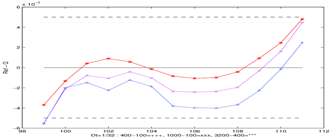
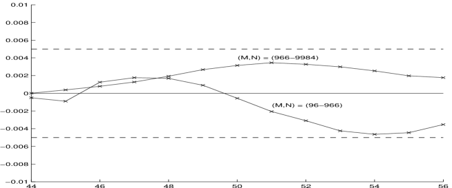
We follow the guidelines of the methodology introduced in [44]: we compute the crude quantized premium for two sizes and , then proceed a space Romberg -extrapolation. Finally, we make a -linear interpolation based on the (Asian) forward moneyness (like in [44]) and the Asian Call-Put parity formula
The anchor strikes and of the extrapolation are chosen symmetric with respect to the forward moneyness. At , the Call is deep out-of-the-money: one uses the Romberg extrapolated computation; at the Call is deep in-the-money: on computes the Call by parity. In between, one proceeds a linear interpolation in (which yields the best results, compared to other extrapolations like the quadratic regression approach).
 |
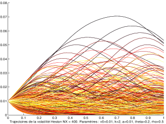 |
Parameters of the Heston model: , , , , , .
Parameters of the option portfolio: , (13 strikes).
The reference price has been computed by a trial Monte Carlo simulation (including a time Romberg extrapolation of the Euler scheme with ).
The differential equations (18) are solved with the parameters of the quantization cubature formulae , with couples of quantization levels , , .

Functional Quantization can compute a whole vector (more than ) option premia for the Asian option in the Heston model with cent accuracy in less than second (implementation in on a processor).
Further numerical tests carried out or in progress with the - model and with the model (Asian, vanilla European options) show the same efficiency. Furthermore, recent attempt to quantize the volatility process and the asset dynamics at different level of quantizations seem very promising in two directions: reduction of the computation time and increase of the robustness of the method to parameter change.
9.3 Comparison: optimized quantization (optimal) product quantization
 |
The comparison is balanced and probably needs some further in situ experiments since it may depend on the modes of the computation. However, it seems that product quantizers (as those implemented in [44]) are from up to times less efficient than optimal quantizers within our range of application (small values of ). On the other hand, the design of product quantizer from -dim scalar quantizers is easy and can be made from some light elementary “bricks” (the scalar quantizer up to and the optimal allocation rules). Thus, the whole set of data needed to design all optimal product quantizers up to is approximately whereas one optimal quantizer with size …
10 Universal quantization rate and mean regularity
The following theorem points out the connection between functional quantization rate and mean regularity of from to .
Theorem 10.1
([33] (2005)) Let be a stochastic process. If there is and such that
for some positive real constant , then
The proof is based on a constructive approach which involves the Haar basis (instead of - basis), the non asymptotic version Zador Theorem and product functional quantization. Roughly speaking, we use the unconditionality of the Haar basis in every (when ) and its wavelet feature its ability to “code” the path regularity of a function on the decay rate of its coordinates.
Examples (see [33]): -dimensional Itô processes (includes -dim diffusions with sublinear coefficients) with .
General Lévy process with Lévy measure with square integrable big jumps. If has a Brownian component, then , otherwise if where (Blumenthal-Getoor index of ), then . This rate is the exact rate
for many classes of Lévy processes like symmetric stable processes, Lévy processes having a Brownian component, etc (see [33] for further examples).
When is a compound Poisson processes, then and one shows, still with constructive methods, that
which is in-between the finite and infinite dimensional settings.
11 About lower bounds
In this overview, we gave no clue toward lower bounds although most of the rates we mentioned are either exact () or sharp () (we tried to emphasize the numerical aspects). Several approaches can be developed to get some lower bounds. Historically, the first one was to rely on subadditivity property of the quantization error derived from self-similarity of the distribution: this works with the uniform distribution over but also in an infinite dimensional framework (see [12] for the fractional Brownian motion).
A second approach consists in pointing out the connection with the Shannon-Kolmogorov entropy (see [29]) using that the entropy of a random variable taking at most values is at most .
A third connection can be made with small deviation theory (see [9], [19] and [33]). Thus, in [19], a connection is established between (functional) quantization and small ball deviation for Gaussian processes. In particular this approach provides a method to derive a lower bound for the quantization rate from some upper bound for the small deviation problem. A careful reading of the proof of Theorem 1.2 in [19] shows that this small deviation lower bound holds for any unimodal (w.r.t. ) non zero process. To be precise: assume that is -unimodal there exists a real such that
For centered Gaussian processes (or processes “subordinated” to Gaussian processes) this follows from the Anderson Inequality (when ). If
for some increasing unbounded function , then
| (21) |
This approach is efficient in the non quadratic case as emphasized in [33] where several universal bounds are shown to be optimal using this approach.
Acknowledgement. I thank S. Graf, H. Luschgy J. Printems and B. Wilbertz for all the fruitful discussions and collaborations we have about functional quantization.
References
- [1] Abaya, E.F. and Wise, G.L. (1982). On the existence of optimal quantizers. IEEE Trans. Inform. Theory, 28, 937-940
- [2] Abaya, E.F. and Wise, G.L. (1984). Some remarks on the existence of optimal quantizers. Statistics and Probab. Letters, 2, 349-351.
- [3] Benveniste, A., Métivier, M. and Priouret, P. (1990). Adaptive algorithms and stochastic approximations, Translated from the French by Stephen S. Wilson. Applications of Mathematics 22, Springer-Verlag, Berlin, 365 pp.
- [4] N. Bouleau, D. Lépingle (1994). Numerical methods for stochastic processes, Wiley Series in Probability and Mathematical Statistics: Applied Probability and Statistics. A Wiley-Interscience Publication. John Wiley & Sons, Inc., New York, 359 pp. ISBN: 0-471-54641-0.
- [5] Bucklew, J.A. and Wise, G.L. (1982). Multidimensional asymptotic quantization theory with power distortion. IEEE Trans. Inform. Theory, 28(2), 239-247.
- [6] Cohort, P. (1998). A geometric method for uniqueness of locally optimal quantizer. Pre-print LPMA-464 and Ph.D. Thesis, Sur quelques problèmes de quantification, 2000, Univ. Paris 6.
- [7] Cuesta-Albertos, J.A., Matrán, C. (1988). The strong law of large numbers for -means and best possible nets of Banach valued random variables, Probab. Theory Rel. Fields 78, 523-534.
- [8] Delattre, S., Fort, J.-C. and Pagès, G. (2004). Local distortion and -mass of the cells of one dimensional asymptotically optimal quantizers, Communications in Statistics, 33(5), 1087-1118.
- [9] Dereich, S., Fehringer, F., Matoussi, A. and Scheutzow, M. (2003). On the link between small ball probabilities and the quantization problem for Gaussian measures on Banach spaces, J. Theoretical Probab., 16, pp.249-265.
- [10] Dereich, S. (2005). The coding complexity of diffusion processes under -norm distortion, pre-print.
- [11] Dereich, S. (2005). The coding complexity of diffusion processes under supremum norm distortion, pre-print.
- [12] Dereich, S., Scheutzow, M. (2006). High resolution quantization and entropy coding for fractional Brownian motions, Electron. J. Probab., 11, 700-722.
- [13] Doss H. (1977). Liens entre équations différentielles stochastiques et ordinaires, Ann. I.H.P., section B, 13(2), 99-125.
- [14] Fleischer, P.E. (1964). Sufficient conditions for achieving minimum distortion in a quantizer. IEEE Int. Conv. Rec., part I, 104-111.
- [15] Gersho, A. and Gray, R.M. (1992). Vector Quantization and Signal Compression. Kluwer, Boston.
- [16] Fort, J.-C. and Pagès, G. (2004). Asymptotics of optimal quantizers for some scalar distributions, Journal of Computational and Applied Mathematics, 146, 253-275, 2002.
- [17] Graf, S. and Luschgy, H. (2000). Foundations of Quantization for Probability Distributions. Lect. Notes in Math. 1730, Springer, Berlin, 230p.
- [18] Graf, S. and Luschgy, H. (2005). The point density measure in the quantization of self-similar probabilities. Math. Proc. Cambridge Phil. Soc.. 138, 513-531.
- [19] Graf, S., Luschgy H. and Pagès, G. (2003). Functional quantization and small ball probabilities for Gaussian processes, J. Theoret. Probab., 16(4), 1047-1062.
- [20] Graf, S., Luschgy, H., Pagès, G. (2007). Optimal quantizers for Radon random vectors in a Banach space, J. of Approximation Theory, 144, 27-53.
- [21] Graf, S., Luschgy, H. and Pagès, G. (2006). Distortion mismatch in the quantization of probability measures, to appear in ESAIM P&S.
- [22] Heston, S.L. (1993). A closed-form solution for options with stochastic volatility with applications to bond and currency options, The review of Financial Studies, 6(2), 327-343.
- [23] Kieffer, J.C. (1983). Uniqueness of locally optimal quantizer for -concave density and convex error weighting functions, IEEE Trans. Inform. Theory, 29, 42-47.
- [24] Kieffer, J.C. (1982). Exponential rate of convergence for Lloyd’s Method I, IEEE Trans. Inform. Theory, 28(2), 205-210.
- [25] Kushner, H. J., Yin, G. G. (2003). Stochastic approximation and recursive algorithms and applications. Second edition. Applications of Mathematics 35. Stochastic Modelling and Applied Probability. Springer-Verlag, New York, 474p.
- [26] Lamberton, D. and Pagès, G. (1996). On the critical points of the -dimensional Competitive Learning Vector Quantization Algorithm. Proceedings of the ESANN’96, (ed. M. Verleysen), Editions D Facto, Bruxelles, 97-106.
- [27] Lapeyre, B., Sab, K. and Pagès, G. (1990). Sequences with low discrepancy. Generalization and application to Robbins-Monro algorithm, Statistics, 21(2), 251-272.
- [28] Lejay, A. (2003). An introduction to rough paths, Séminaire de Probabilités XXXVII, Lecture Notes in Mathematics 1832, Stringer, Berlin, 1-59.
- [29] Luschgy, H., Pagès, G. (2002). Functional quantization of Gaussian processes, Journal of Functional Analysis, 196(2), 486-531.
- [30] Luschgy, H., Pagès, G. (2004). Sharp asymptotics of the functional quantization problem for Gaussian processes, The Annals of Probability, 32(2), 1574-1599.
- [31] Luschgy, H., Pagès, G. (2006). Functional quantization of a class of Brownian diffusions: A constructive approach, Stochastic Processes and Applications, 116, 310-336.
- [32] Luschgy, H., Pagès, G. (2005). High-resolution product quantization for Gaussian processes under sup-norm distortion, pre-pub LPMA-1029, forthcoming in Bernoulli.
- [33] Luschgy, H., Pagès, G. (2006). Functional Quantization Rate and mean regularity of processes with an application to Lévy Processes, pre-print LPMA-1048.
- [34] Luschgy, H., Pagès, G. (2007). Expansion of Gaussian processes and Hilbert frames, technical report.
- [35] Luschgy, H., Pagès, G. and Wilbertz, B. (2007). Asymptotically optimal quantization schemes for Gaussian processes, in progress.
- [36] Mrad, M., Ben Hamida, S. (2006). Optimal Quantization: Evolutionary Algorithm Stochastic Gradient, Proceedings of the 9th Joint Conference on Information Sciences.
- [37] Newman, D.J. (1982). The Hexagon Theorem. IEEE Trans. Inform. Theory, 28, 137-138.
- [38] H. Niederreiter (1992) Random Number Generation and Quasi-Monte Carlo Methods, CBMS-NSF regional conference series in Applied mathematics, SIAM, Philadelphia.
- [39] Pagès, G. (1993). Voronoi tessellation, space quantization algorithm and numerical integration. Proceedings of the ESANN’93, M. Verleysen Ed., Editions D Facto, Bruxelles, 221-228.
- [40] Pagès, G. (1997). A space vector quantization method for numerical integration, J. Computational and Applied Mathematics, 89, 1-38.
- [41] Pagès, G. (2000). Functional quantization: a first approach, pre-print CMP12-04-00, Univ. Paris 12.
- [42] Pagès, G., Pham, H. and Printems, J. (2003). Optimal quantization methods and applications to numerical methods in finance. Handbook of Computational and Numerical Methods in Finance, S.T. Rachev ed., Birkhäuser, Boston, 429p.
- [43] Pagès, G., Printems, J. (2003). Optimal quadratic quantization for numerics: the Gaussian case, Monte Carlo Methods and Appl., 9(2), 135-165.
- [44] Pagès, G., Printems, J. (2005). Functional quantization for numerics with an application to option pricing, Monte Carlo Methods and Appl., 11(4), 407-446.
- [45] Pagès, G., Printems, J. (2005). Website devoted to vector and functional optimal quantization: www.quantize.maths-fi.com.
- [46] Pagès, G., Sellami, A. (2007). Convergence of multi-dimensional quantized SDE’s. In progress.
- [47] G. Pagès, Y.J. Xiao (1988) Sequences with low discrepancy and pseudo-random numbers: theoretical results and numerical tests, J. of Statist. Comput. Simul., 56, 163-188.
- [48] Pärna, K. (1990). On the existence and weak convergence of -centers in Banach spaces, Tartu Ülikooli Toimetised, 893, 17-287.
- [49] Pollard, D. (1982). Quantization and the method of -means. IEEE Trans. Inform. Theory, 28(2), 199-205.
- [50] P.D. Proinov (1988). Discrepancy and integration of continuous functions, J. of Approx. Theory, 52, 121-131.
- [51] Revuz, D., Yor, M. (1999). Continuous martingales and Brownian motion, Third edition. Grundlehren der Mathematischen Wissenschaften [Fundamental Principles of Mathematical Sciences], 293, Springer-Verlag, Berlin, 1999, 602 p.
- [52] K.F. Roth (1954). On irregularities of distributions, Mathematika, 1, 73-79.
- [53] Tarpey, T., Kinateder, K.K.J. (2003). Clustering functional data, J. Classification, 20, 93-114.
- [54] Tarpey, T., Petkova, E., Ogden, R.T. (2003). Profiling Placebo responders by self-consistent partitioning of functional data, J. Amer. Statist. Association, 98, 850-858.
- [55] Trushkin, A.V. (1982). Sufficient conditions for uniqueness of a locally optimal quantizer for a class of convex error weighting functions, IEEE Trans. Inform. Theory, 28(2), 187-198.
- [56] Wilbertz, B. (2005). Computational aspects of functional quantization for Gaussian measures and applications, diploma thesis, Univ. Trier.
- [57] Zador, P.L. (1963). Development and evaluation of procedures for quantizing multivariate distributions. Ph.D. dissertation, Stanford Univ.
- [58] Zador, P.L. (1982). Asymptotic quantization error of continuous signals and the quantization dimension. IEEE Trans. Inform. Theory, 28(2), 139-149.