Turbulence Models Generator.

Abstract

In this paper we explore a possibility that all transport turbulent models are contained in a coarse-grained kinetic equation. Building on a recent work by H.Chen et al (2004), we account for fluctuations of a single -point probability density in turbulence, by introducing a“two-level” ( ${\bf c,v}$)-phase-space, separating microscopic (${\bf c^{\prime}\equiv c_{micro}=c-v}$) and hydrodynamic (${\bf v^{\prime}=v-V}$) modes. Unlike traditional kinetic theories, with hydrodynamic approximations derived in terms of small deviations from thermodynamic equilibrium, the theory developed in this work, is based on a far- from -equilibrium isotropic and homogeneous turbulence as an unperturbed state. The expansion in dimensionless rate of strain leads to a new class of turbulent models, including the well-known ${\cal K}-{\cal E}$, Reynolds stress and all possible nonlinear models. The role of interaction of the fluxes in physical space with the energy flux across the scales, not present in standard modeling, is demonstrated on example of turbulent channel flow. To close the system, neither equation for turbulent kinetic energy nor information on pressure-velocity correlations, contained in the derived coarse-grained kinetic equation, are needed.

1–10 ?? and in revised form ??

1 Introduction

In this paper we revisit an old and all-important problem of turbulent modeling. The problem, first formulated in terms of images borrowed from kinetic theory by Prandtl (1925), was later developed by Kolmogorov (1942), Launder and Spaulding (1974) and many of their followers. The success of these semi-empirical approaches can hardly be overestimated: with development of powerful computers turbulent modeling became an important part of scientific and engineering design process. Still, these models, involving low -order time - derivatives and low powers of dimensionless rate of strain, are less effective in describing strongly sheared and rapidly distorted flows where the dimensionless rate of strain is not too small. To improve performance, various non-linear models, pioneered by Speziale (1987), accounting for the next order in powers of the rate of strain, have been proposed. Since the second-order trancation of a lacking-small -parameter expansion is problematic, these models had a mixed success. (The role of the large-eddy simulations (LES) in description of complex flows will be discussed in Conclusions. )

The attempts to systematically derive turbulence transport models from the Navier-Stokes equations (NS), based on renormalized Wyld’s perturbation expansions (RNG (Yakhot/ Smith et al (1992), Rubinstein and Barton (1990)), double expansion (Yakhot et al (1992)), DIA (Yoshizawa (1987)), were relatively successful and the resulting equations found their place in engineering. It became clear soon that resummation of the series was impractical and the approach was restricted to the low- orders.

It has been shown recently by H. Chen et al (2004) that the turbulence models, derived by application of the Chapman-Enskog expansion (CE) to a model kinetic (Boltzmann-BGK) equation written for hydrodynamic modes, are similar to those previously obtained from the Wyld (1961) expansion, applied directly to the Navier-Stokes equations. The main result of Chen et al (2004) can be stated as follows: the perturbation theory, leading from kinetic equation to the Navier-Stokes (NS) equations, generates the well-known turbulence models if, instead of the relaxation time $\tau=\nu_{0}/\theta=const$ of kinetic theory, one writes $\tau_{T}\approx K/{\cal E}$ and represents the temperature $\theta$ as $\theta=K$. Here $K$ and ${\cal E}$ are the mean turbulent kinetic energy and dissipation rates, respectively. Thus, the formal superficial similarity between the two perturbation expansions has been established. This result means that, in principle, the models of an arbitrary non-linearity and complexity, which we even cannot explicitly write down, are contained in a simple kinetic equation.

In this work, we would like to reformulate the procedure developed in Chen (2004) by taking into account both microscopic and hydrodynamic modes. The coarse-grained kinetic equation for hydrodynamic modes is then obtained by integrating out the fast microscopic variables. To achieve this goal, we had to substantially redefine the expansion procedure and, as a result, obtain a qualitatively new class of turbulence models.

1.1 The Boltzmann -BGK equation.

Kinetic theory for a low-density gas is based on the Boltzmann equation

$$\frac{\partial f}{\partial t}+{\bf c\cdot\nabla}f={\cal C}(f)$$ (1)

for a single particle distribution function $f({\bf c},{\bf x},t)$, where collision integral

$${\cal C}(f)=\int w^{\prime}(f^{\prime}f^{\prime}_{1}-f\;f_{1})\;d\Gamma_{1}d\Gamma^{\prime}d\Gamma^{\prime}_{1}=\int|c_{rel}|(f^{\prime}f^{\prime}_{1}-f\;f_{1})d\sigma d^{3}p_{1}\equiv i_{in}-i_{out}$$ (2)

If the system Hamiltonin is known, this equation can be derived directly from the Liuville theorem. Here the element of the phase -space volume $d\Gamma=d{\bf x}d{\bf p}$ and $|c_{rel}|=|{\bf c_{1}-c}|$ is the relative velocity of colliding particles. If the intermolecular distance is $\lambda>>a$ where $a$ is the length-scale of intermolecular interaction, the strait particle trajectories between collisions are assumed in deriving expression (1.2). The probability density functions in (1.2) are $f^{\prime}=f^{\prime}(r,{\bf c^{\prime}},t)$ and $f^{\prime}_{1}=f^{\prime}(r,{\bf c^{\prime}_{1}},t)$. Since in accord with the theory of elastic collisions, the velocities ${\bf c^{\prime},\ c^{\prime}_{1}}$ are expressed in terms of ${\bf c,\ c_{1}}$, the integration in (1.2) is carried out over the phase space $\Gamma_{1}$ only. The relaxation -time approximation (RTA):

$${\cal C}=-\frac{f-f^{eq}}{\tau}$$ (3)

where $f^{eq}$ is the distribution function in thermodynamic equilibrium and $\tau$ is a properly chosen relaxation time, is an often used anztaz, mentioned in Landau and Lifshitz (1981) as a ”rough estimate of the ( Boltzmann) collision integral” (1.2). Still, recent implementations of this approximation in the so called ”Lattice Boltzmann” numerical codes, led to a remarkable success in simulating a wide variety of extremely complex fluid flows. As of today, the approach has been tested on basically all examples of classic laminar flows (Benzi (1992), Chen (1998), Succi (2001)). The robustness, speed and simplicity of the method, made it an attractive tool for both theoretical investigations and engineering design.

Even more spectacular, and somewhat unexpected, is success enjoyed by the Lattice Boltzmann method in simulating complex turbulent flows (H. Chen (2003)). In this application, the relaxation time $\tau$ is expressed in terms of hydrodynamic observables: $\tau\approx{\cal K}/{\cal E}$ , where turbulent kinetic energy is ${\cal K}=v_{rms}^{2}/2$ and the mean dissipation rate is ${\cal E}=\nu\overline{(\frac{\partial v_{i}}{\partial x_{j}})^{2}}$. In this case, in the first order of the Chapman-Enskog (CE) expansion one obtains the well-known ${\cal K}-{\cal E}$ model with the non-linear ${\cal K}-{\cal E}$ model appearing in the next order (Chen et al (2004)). In addition to speed and simplicity, the most attractive feature of this type of turbulence modeling is that it does not require theory of pressure-velocity correlations which, in complex flows, is an extremely difficult, still unsolved, problem.

Typically, derivation of hydrodynamic Navier-Stokes equations from kinetic theory is based on a few assumptions. 1.  If spatial gradients of mean velocity, density and temperature are equal to zero, the gas is assumed in thermodynamic equilibrium; 2.  Expansion in powers of dimensionless rate of strain $\eta\equiv\eta_{ij}=\tau S_{ij}$ where $S_{ij}=\frac{1}{2}(\frac{\partial V_{i}}{\partial x_{j}}+\frac{\partial V_{j}}{\partial x_{i}})$ leads to transport equations describing various physical phenomena.

The equations, derived this way can be used to fully describe large Reynolds number turbulent flows requiring at least $N\approx Re^{3}$ number of degrees of freedom. In the flows of practical importance this number is huge and therefore, the value of a coarse graining procedure leading to turbulence models can hardly be overestimated .

It has been shown (Yakhot et al (1992) ) that the systematic derivation of turbulence models directly from the Navier-Stokes equations, can be formulated in terms of Wyld’s (1961) diagramamtic expansion in two dimensionless parameters: the Reynolds number $Re=u_{rms}L/\nu_{0}$ and, familiar from kinetic theory, dimensionless rate of strain $\eta=\tau_{T}S_{ij}$. The first expansion is responsible for description of isotropic and homogeneous turbulence with the non-zero energy flux across the scales and the second  -  for the non-zero spatial fluxes and flow structures. Due to proliferation of tensorial indices in the high-order contributions, the resummation of the expansion is an extremely difficult task and it has been conjectured by Polyakov (2001) in the middle of seventies that it may result in a kinetic equation containing all terms of Wyld’s series. If this is true, a turbulence model of an arbitrary non-linearity and complexity may be contained in a relatively simple kinetic equation. The most important and interesting feature of this system is that, unlike equilibrium, the $\eta=0$ state of isotropic and homogeneous turbulence is not flux- free but involves a large $O(1)$ energy flux across the scales. Thus, to derive turbulence models, it is desirable to develop a kinetic approach not based on the equilibrium, flux-free, zero-order state.

In this paper we, building upon a remarkable work of H. Chen et al (2004), consider both turbulent (hydrodynamic) and thermal (microscopic) velocity fluctuations as governed by the Boltzmann -BGK kinetic equation. Since microscopic and hydrodynamic fluctuations occupy their respective fractions of the phase-space, this equation is formally defined on a somewhat enlarged phase-space. The coarse-graining, eliminates the small-scale fast microscopic fluctuations and restores the six-dimensional space, leading to the kinetic equation for the large-scale (turbulent) velocity component only. In this case, the zero-order, zero-mean-spatial-gradient state is not an equilibrium but that of isotropic and homogeneous turbulence characterized by a finite energy flux across the scales. The Chapman-Enskog expansion applied to this state leads to a novel set of turbulence models of arbitrary nonlinearity.

This paper is organized as follows. In the next Section we, for the sake of clarity and continuity, describe traditional derivation of hydrodynamic approximations from kinetic equation and briefly outline the way turbulence models appear from the NS equations. In Section 3, which is most important for the present development, we introduce the non-equilibrium kinetic equation and the zero-order pdf for isotropic and homogeneous turbulence, both defined on an enlarged phase-space. In Section 4, the finite energy flux is defined as a dynamic constraint and it is shown that the introduced in Section 3 non-equilibrium pdf is indeed a solution to non-equilibrium equation which conserves the total kinetic energy of a system. Finally, in Section 5, the coarse-grained kinetic equation for hydrodynamic modes is derived. It is shown in Sections 6 and 7, that the CE expansion, leads to transport equations for both turbulent velocity field and kinetic energy. In Section 8, choosing a proper relaxation time, we show that our kinetic equation contains the well known K-E , Reynolds stress and non-linear models. In addition, this simple equation contains turbulent models of an arbitrary non-linearity and complexity. Some new effects, originating from interaction of spatial fluxes with the energy flux (cascade) are identified. Summary and conclusions are presented in Section 9.

1.2 Equilibrium.

In equilibrium, with all temporal and spatial gradients equal to zero, the left side of kinetic equation (1.1),(1.2) is equal to zero and the remaining equation ${\cal C}=0$ has a solution:

$$f^{eq}=constant\times e^{-\frac{E(\Gamma)}{\theta}}$$ (4)

where the energy $E(\Gamma)$ is conserved in the process of collision, i.e. $E^{\prime}+E^{\prime}_{1}=E+E_{1}$ and the temperature $\theta=const$. For a gas moving with the constant velocity ${\bf V}$, the solution is:

$$f^{eq}=const\times e^{-\frac{E(\Gamma)-{\bf p\cdot V}}{\theta}}$$ (5)

This solution is clear if we introduce internal energy $\epsilon_{in}$ and write

$$E(\Gamma)=\epsilon_{in}+\frac{mc^{2}}{2}$$ (6)

In a frame of reference moving with velocity ${\bf V}$, we have

$$f^{eq}=constant\times e^{\frac{\mu-\epsilon_{in}}{\theta}}e^{-\frac{m({\bf c-V})^{2}}{2\theta}}$$ (7)

In deriving transport approximation, one expands the probability density powers the large-scale field (LL) ${\bf V}\approx{\bf V_{0}}+\frac{\partial{\bf V}}{\partial x_{i}}x_{i}$. The constant component $V_{0}=const$ can be removed by the Galileo transformation and only derivatives of the large scale field ${\bf V}$ are relevant.

2 Hydrodynamic approximation

In this Section we, for the sake of clarity and continuity, briefly describe the main steps leading from the Boltzmann equation to hydrodynamic approximations.

Classic derivation of transport approximations starts with the Boltzmann equation (1.1), (1.2) or (1.3) and equilibrium pdf

$$f^{eq}=\frac{\rho}{(2\pi\theta)^{\frac{3}{2}}}\exp(-\frac{({\bf c-v}({\bf x},t))^{2}}{2\theta})$$ (8)

In this Section we denote velocity of the frame of reference ${\bf v}({\bf x},t)$ which is a physical (not phase-space variable). In what follows we restore the notation $({\bf V})$ used above. This should not lead to any difficulty. The equilibrium pdf is obtained from equation ${\cal C}(f^{eq})=0$, which is valid locally, so that the hydrodynamic field ${\bf v({\bf x},t})$ can be a slow varying function of time and space coordinates. In addition, the conservation laws and the symmetries of collision integral give:

$$\int{\cal C}d{\bf c}=\int{\cal C}(f){\bf c}d{\bf c}=0$$ (9)

Introducing the fluid density $\rho=\int f({\bf v})d{\bf v}$ and integrating (1.1)-(1.2) over ${\bf c}$ leads to the continuity equation:

$$\frac{\partial\rho}{\partial t}+\nabla\cdot\rho{\bf v}=0$$ (10)

Multiplying (1.1)-(1.2) by ${\bf c}$ with subsequent integration over the phase space yields :

$$\frac{\partial\rho v_{j}}{\partial t}+\partial_{i}\rho v_{j}v_{i}+\partial_{i}\sigma_{ij}=0$$ (11)

where the stress tensor is : $\sigma_{ij}=\overline{\rho(c_{i}-v_{i})(c_{j}-v_{j})}$. In thermodymanic equilibrium, the stress-tensor is evaluated readily with the distribution function $f^{eq}$ from (2.1) giving $\sigma_{ij}|_{eq}=\rho\theta\delta_{ij}$, so that combining this with the ideal gas equation, gives:

$$\frac{\partial v_{j}}{\partial t}+v_{i}\partial_{i}v_{j}-\frac{1}{\rho}\nabla p=0$$ (12)

In what follows $\overline{A}|_{eq}\equiv\int Af^{eq}d{\bf c}$. Defining $\theta=\frac{1}{d}\overline{(c_{i}-v_{i})^{2}}$, we obtain:

$$\frac{\partial\theta}{\partial t}+\nabla_{i}\rho v_{i}\theta+\frac{1}{d}\nabla_{i}\rho\overline{(c_{i}-v_{i})(c_{j}-v_{j})^{2}}+\frac{2}{d}\rho\overline{(c_{i}-v_{i})(c_{j}-v_{j})}S_{i,j}=0$$ (13)

On the equilibrium pdf $f^{eq}$, $\sigma^{eq}_{ij}=\theta\delta_{ij}$ and the third-order in fluctuations contribution to (2.6) is equal to zero.

2.1 Turbulence modeling.

The nature of the large-scale hydrodynamic field ${\bf v}$ in (2.4) has not been specified. The problem of turbulence modeling is formulated as follows: let the velocity field ${\bf v}={\bf V}+{\bf v^{\prime}}$ where $\overline{{\bf v^{\prime}}}=0$ and $\overline{{\bf v}}={\bf V}$. Our goal is to derive the equation for the large-scale slow field ${\bf V}$. The above decomposition gives:

$$\frac{\partial{\bf V}}{\partial t}+{\bf V\cdot\nabla V}+\overline{{\bf v^{\prime}\cdot\nabla v^{\prime}}}+\frac{1}{\rho}\nabla\cdot\sigma=0$$ (14)

or

$$\frac{\partial{\bf V}}{\partial t}+{\bf V\cdot\nabla V}+\frac{1}{\rho}\nabla\cdot(\sigma+\sigma_{v})-\overline{{\bf v^{\prime}\nabla\cdot v^{\prime}}}=0$$ (15)

where

$$\sigma_{ij,v}=\overline{(v-V)_{i}(v-V)_{j}}$$ (16)

Now we need a theory or at least set of rules to express both stress $\sigma$ and the Reynolds stress $\overline{{\bf v^{\prime}\cdot\nabla v^{\prime}}}$ in terms of the large-scale field ${\bf V}$ and its derivatives. This program has been systematically developed in Yakhot et al (1992), Smith et al (1992). The method consists of a few steps: 1. In the first order, the stress tensor $\sigma_{ij}\approx 2\nu_{0}S_{ij}$. This leads to the Navier-Stokes equations (NS). 2.   Add a statistically isotropic and homogeneous stirring force to the right side of the NS. This force generates an $O(1)$ energy flux ${\cal P}=\overline{{\bf f\cdot v^{\prime}}}={\cal E}$ across scales. In the case of a free turbulence with the total kinetic energy $K$, prepared as an initial condition, the energy balance reads $\partial_{t}K=-{\cal E}$. 3.  Use Wyld’s (1961) expansion to eliminate small-scale velocity fluctuations. It has been shown (Yakhot et al (1992)) that development of turbulent models involves a double expansion in powers of two dimensionless parameters: the Reynolds number $Re=v^{\prime}_{rms}L/\nu$ and rate of strain $\eta_{ij}\equiv\eta=\tau S_{i,j}$ where $\tau_{T}$ is the relaxation time of turbulent fluctuation. The expansion in Re leads to the fixed point $Re_{*}\approx v^{\prime}_{rms}L/\nu_{T}=const$, corresponding to the zero- spatial -gradient state of isotropic and homogeneous turbulence which serves a a ground state for the additional expansion in powers $\eta$. The first expansion accounts for the non-zero energy flux of isotropic and homogeneous turbulence while the second -  gives rise to the not zero mean velocity field and various fluxes. In the first order of the $\eta$-expansion one derives a variant of ${\cal K}-{\cal E}$ model, in the second -the Reynolds stress model and non-linear models etc. It is important that the second order $O(\nu_{T}^{2}/K{\bf S\cdot S})$ terms of the non-linear turbulent models, are well known from kinetic theory as next-order in the Chapman-Enskog expansion corrections to the Navier-Stokes equations (Landau-Lifshitz (1981) ). This fact establishes similarities between Wyld’s expansion of the NS equations and the CE expansion of kinetic theory. While, one can formally write each term of the $\eta$-expansion, resummation of an infinite series is totally out of reach.

3 Formulation in terms of kinetic equation.

In turbulent flows, the velocity field is characterized by three correlation lengths (Landau and Lifshitz (1959), Frisch (1996)): 1.   microscopic mean -free path $r\approx\lambda\approx c_{s}\tau$, where $c_{s}$ is the speed of sound and $\tau$ is the microscopic relaxation time; 2. hydrodynamic inertial interval $\eta_{K}\approx LRe^{-\frac{3}{4}}\leq r\leq L$, where both large-scale forcing and viscous effects can be neglected and 3.  nonuniversal, geometry-dependent, energy-production range $r\geq L$. We denote three velocity fields corresponding to these intervals as ${\bf c^{\prime}\equiv c_{micro}=c-v;~{}v^{\prime}=v-V;~{}V}$, respectively. (See Fig.1). Locally, at the scales $r\approx\lambda$, the system is in thermodynamic equilibrium so that the ${\bf c_{micro}}$-field obeys Maxwell (Gibbs) statistics.

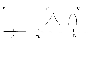
Figure 1: Scale and velocity field intervals in turbulence: 1.  Energy range : $r>L$ (V ); 2. Inertial range: $\eta_{K}\leq r\leq L$ (v’=v-V). PDFs: $r\approx L$ (Gausss); $r\ll L$ (Multifractal); $r\leq\lambda$ (Microscopic) (c’=c-v ).

Hydrodynamic approximations follow elimination (small-scale averaging) of modes from the interval $r\leq\lambda\approx c_{s}\tau$, where $\tau$ is the relaxation time characterizing dynamics of small perturbations from thermodynamic equilibrium. After that, the turbulence models are derived by averaging the Navier-Stokes equations in the interval $\eta_{K}\leq r\leq L$. We do not doubt the ability of the Navier-Stokes equations fully describe turbulent flow of arbitrarily large Reynolds number. In this case, since the number of excited modes is at least $O(Re^{9/4})$, the computational cost of these direct simulations (DNS) is very high. Our concern here is with derivation of the coarse-grained equations (turbulence models) for partial representation of turbulence in the interval $r\approx L$, which is hard to obtain from hydrodynamics. In other words, in this work we are interested in the mode-elimination from the interval $0\leq r\leq L$ applied directly to the Boltzmann equation. If successful, this way we will obtain the coarse-grained kinetic equation, containing, as a hydrodynamic approximation, all possible turbulence models, which are very hard to derive from the Navier-Stokes equation. In particular, we are interested in equations of motion for the coarse-grained or filtered velocity field which includes only a small fraction of hydrodynamic modes corresponding to the top of inertial range, i.e. $r\approx L$. Whatever the filtering procedure, the coarse-grained fields are obtained from the full fields by averaging over flow volumes of linear dimension $r\approx\Delta<L$, where $\Delta$ is the filtering scale or over the modes ${\bf v(k)}$ with $k>1/\Delta$ in a Fourier space. Also, one can define a coarse - grained field as:

$${\bf v}({\bf x})\approx\frac{1}{{\cal R}({\bf x})}\int_{{\cal R}}{\bf v}({\bf x^{\prime}})\ d{\bf x^{\prime}}$$

where the integration is carried out over the volume ${\cal R}\approx\Delta^{3}$ centered about the point ${\bf x}$ or

$${\bf v}({\bf x})\approx\int{\bf v}({\bf x^{\prime}})F(|{\bf x-x^{\prime}}|/\Delta)\ d{\bf x^{\prime}}$$

where $F$ is a filter function. We see that the coarse-grained velocity field is a multipoint construction and evaluation of high-order moments is not a simple task. Moreover, spatial velocity derivatives are defined on a cut-off as:

$$\partial_{x}v=(v(x+\Delta_{x})-v(x))/\Delta_{x}$$

and, if $\Delta\ll L$, their moments, called structure functions, obey multifractal statistics. The inertial range multifractality (anomalous scaling ) means that the moments of different orders are independent of each other. As a result, the full statistical description of velocity field involves a large, infinite in the limit $Re\rightarrow\infty$, number of independent parameters. This makes an accurate coarse-graining with the filter (mesh) size $\Delta<<L$ basically impossible.

The situation changes dramatically in the limit $\Delta\rightarrow L$. It is a well-established, though not well-understood, fact that at the scales $r=\Delta\approx L$, both the turbulent velocity fields ${\bf v^{\prime}=v-V}$ and $\delta{\bf v^{\prime}}={\bf v^{\prime}}({\bf x+\Delta})-{\bf v^{\prime}}({\bf x})$ obey close- to- gaussian statistics. Moreover, it was demonstrated by Schumacher et al (2007) that in the low-Reynolds number turbulence, the velocity derivatives, too, are Gaussian random variables. If this is so, the entire large-scale field can be accurately described in terms of the second-order moment only. Our goal is to derive a coarse - grained equation for the modes ${\bf v^{\prime}}$ fluctuating on the scales $r\approx L$. In the standard turbulence modeling, this is operationally achieved by introducing a large “effective viscosity” $\nu_{T}\approx u_{rms}L$, where $2K=u^{2}_{rms}\approx\frac{3}{2}C_{K}L^{2}$, into the Navier-Stokes equations. Due to a particular choice of viscosity $\nu_{T}\gg\nu_{0}$, the small-scale modes ($r\ll L$) are overdamped and the resulting hydrodynamic equations describe large-scale properties ($r\approx L$) of the flow only. The defined this way equation is called “ transport model” as as opposed to the LES models based on an inertial range cut -off $r=\Delta\ll L$. Since the dominant contribution to turbulent kinetic energy is contained in the large -scale fluctuations, we write the zero-order nonequillibrium probability density function in the laboratory reference frame:

$$f^{0}=\frac{\rho}{8\pi^{3}({\cal K}\theta)^{\frac{3}{2}}}\exp(-\frac{({\bf c-v})^{2}}{2\theta})\exp(-\frac{({\bf v-V})^{2}}{2{\cal K}})\equiv f^{0}({\bf v})Q^{0}({\bf c}|{\bf v})$$ (17)

In this expression, both ${\bf c}$ and ${\bf v}$- fields are phase-space variables independent of time and space. Thus, we have temporarily enlarged the phase space from six to nine dimensions. The flow described by the probability density function (3.1) can be perceived as an ensemble of laminar flows each in thermodynamic equilibrium with the fluctuating equilibrium Maxwell-Gibbs probability density. It is clear that: $\int f^{0}d{\bf v}d{\bf c}=\rho$ and $\overline{\bf c}|_{0}\equiv\int cf^{0}d{\bf c}d{\bf v}={\bf V}$ and $\overline{{\bf v}}|_{0}={\bf V}$. In the laminar limit ${\cal K}\rightarrow 0$

$$f^{0}\propto\frac{1}{(2\pi\theta)^{\frac{3}{2}}}\exp(-\frac{({\bf c-v})^{2}}{2\theta})\delta({\bf v-V})$$

and integrating over ${\bf v}$, we recover the expression (2.1). The pdf (3.1), resembling that of a mixture of gases with different temperatures $\theta$ and ${\cal K}$, describes an essentially non-equilibrium state. It will be shown below that (3.1) is a solution to a “nonequilibrium” kinetic equation and this temperature difference is related to the energy flux from hydrodynamic modes to the microscopic ones.

From the above definitions:

$${\bf V}=\overline{\bf v}|_{0}=\int{\bf v}f^{0}({\bf c,v})d{\bf c}d{\bf v}$$

$$\xi^{0}({\bf v})f^{0}({\bf v})=\int{\bf c}f^{0}({\bf c,v})d{\bf c}={\bf v}f^{0}({\bf v})$$

$${\cal K}=\frac{1}{d}\overline{({\bf v-V})^{2}}|_{0}=\frac{1}{d}\int({\bf v-V)}^{2}f^{0}({\bf v,c})d{\bf c}d{\bf v}$$

In what follows, we assume the probability density

$$f({\bf c,v,x},t)=\rho f(\frac{{\bf c-v}}{\sqrt{\theta}},\frac{{\bf v-V}}{\sqrt{{\cal K}}},t)$$ (19)

so that locally $\overline{({\bf c-v})^{2}}=d\theta$ and $\overline{({\bf V-v})^{2}}=d{\cal K}$

The pdf of hydrodynamic velocity field $f({\bf v})$ is obtained from (3.3) by integrating out the microscopic variable ${\bf c}$, i.e.

$$f({\bf v})=\int f({\bf c,v,x},t)d{\bf c}$$ (20)

Our goal is to derive a kinetic equation for $f({\bf v})$ describing turbulent fluctuations only. To achieve this goal, we first increase the original six-dimensional phase space of the previous section (${\bf c,x}$) to the nine-dimensional one (${\bf c,v,x}$) and, eliminating thermodynamic fluctuations, project the nine-dimensional problem to the six-dimensional one $({\bf v,x})$. The advantage of this procedure from the turbulence modeling viewpoint is that while original problem involved $N_{\lambda}\approx\Omega/\lambda^{3}$ number of particles, the coarse-grained one  -  only $N_{L}\approx\Omega/\L^{3}$, where the integral scale $L\gg\lambda$ is the large scale correlation length of turbulence.

Since the fast ${\bf c_{micro}=c-v}$ -field varies on the time scale $\tau\approx\lambda/c_{s}$, where $c_{s}$ stands for the speed of sound, $\overline{{\bf(c-v)\cdot v}}=0$, we can consider these components statistically ortogonal and introduce the continuity equation in the enlarged 9d-phase- space. In this case the Botzmann equation (Landau/Lifshitz (1981)):

$$\frac{\partial f}{\partial t}+{\bf c}\cdot\nabla f=I(f({\bf c,v}))$$ (21)

where $I(f)$ is not yet specified ‘non-equilibrium collision integral’ with $f^{0}({\bf v,c,x},t)$ obtained from equation:

$$\frac{\partial f^{0}}{\partial t}=I(f^{0}({\bf c,v}))\neq 0$$ (22)

with $V=const$ ($S_{ij}=0)$. Thus, in the theory developed below, we abandon the equilibrium pdf (2.1) for the the zero-spatial-gradient state of a gas in favor of the nonequilibrium expression (3.1). The detailed discussion of this point will be given below. Here we just mention that due to the non-zero energy flux across the scales, the kinetic energy of the zero-spatial-gradient ($\eta=0$) turbulent flow decays leading to increase of the gas temperature $\theta$.

4 Finite energy flux as a dynamic constraint.

If a turbulent flow is supported by a large-scale energy input per second ${\cal P}$, by nonlinearity, this energy is transfered to the smallest scales where it is dissipated. It is usually assumed that the nature of the dissipation mechanism is unimportant. On the inertial- range scales, where both energy pumping and dissipation are negligibly small, the dynamics are characterized by the mean energy flux $J={\cal P}={\cal E}$, where ${\cal E}$ is the mean dissipation rate. In case of isotropic and homogeneous turbulence, prepared at initial instant of time with kinetic energy $K(0)$, the energy $K(t)$ decays to zero. Since in this case, all spatial gradients are equal to zero, no mean spatial fluxes are involved in the relaxation process. Unlike equilibrium gas, this strongly non-equilibrium system is characterized by a non-zero constant energy flux across the scales .

It has been shown in a series of extraordinary works by Zakharov et al (1975), (1992), (1984) that, in case of turbulence, the Euler equations, with velocity field written in terms of Clebsch variables, can be represented as a kinetic equation for waves (particles) with the collision integral $I_{C}$ describing the non-linear interactions. It has been shown that, in addition to equilibrium solutions, the equation $I_{C}(n({\bf k}))=0$ for the occupation numbers $n(k)$, playing the role of the pdf in the $k$-space, has solutions corresponding to the non-zero constant fluxes in the wave-number space. The direction of these fluxes is exclusively determined by physics of the problem and peculiarities of non-linear interactions. For example, the mean field approximation developed in Yakhot (1992), led to the Kolomogorov energy spectrum as one of Zakharov’s constant-flux solutions. Thus, unlike thermodynamic equilibrium, the kinetic equation for a zero -mean-gradient turbulent flow must satisfy the flux (energy balance) constraints:

$${\cal P}={\cal E}$$ (23)

valid in the statistically steady state or

$$\frac{\partial{\cal K}}{\partial t}=-\frac{2}{d}{\cal E}$$ (24)

-  in case of decaying turbulence.

The relations (4.2) and (4.3), reflecting the energy balance in a flow, are independent upon the nature of the dissipation mechanism. We split collision integral $I(f)$ into two components: $I_{hi}(f)$ responsible for the non-zero energy flux of isotropic and homogeneous turbulence and $I^{1}(f)$ -  for the spatial fluxes of a general turbulent flow. Since, as was pointed out above, the mean energy flux is a large-scale property, no differential operator can enter the expression. Thus we have: $I(f)=I_{hi}+I^{1}$ and

$$I_{hi}=-\frac{f}{\tau_{hi}}=-[\frac{({\bf v-V})^{2}-d{\cal K}}{d{\cal K}}-\frac{{\cal K}}{\theta}\frac{({\bf v-c})^{2}-d\theta}{d\theta}]\frac{{\cal E}}{{\cal K}}f({\bf c,v})$$ (25)

4.1 Isotropic and homogeneous turbulence.

Now we will show that the zero-order pdf (3.1) is a solution to kinetic equation describing isotropic and homogeneous turbulence. Since in this case, all spatial derivatives are equal to zero, the kinetic equation is:

$$\frac{\partial f^{0}}{\partial t}=I_{hi}$$ (26)

and $\overline{{\bf c}}=\overline{{\bf v}}=0$, $\overline{c^{2}}=d\theta$ and $\overline{v^{2}}=d{\cal K}$. Substituting (3.1) into (3.5)-(3.6) gives:

$$\frac{1}{\theta}(\frac{({\bf v-c})^{2}}{\theta}-d)(\frac{\partial\theta}{\partial t}-\frac{2}{d}{\cal E})=\frac{1}{{\cal K}}(\frac{v^{2}}{{\cal K}}-d)(\frac{\partial{\cal K}}{\partial t}+\frac{2}{d}{\cal E})$$ (27)

This equation, valid for all values of independent parameters $c$ and $v$, can be correct only if:

$$\frac{\partial K}{\partial t}=-{\cal E}$$ (28)

$$\frac{d}{2}\frac{\partial\theta}{\partial t}={\cal E}$$ (29)

Thus, we conclude that the zero-order pdf (3.1) is indeed a solution to the kinetic equation (3.5), (3.6) for isotropic and homogeneous turbulence, subject to the energy constraints (4.1),(4.2). One can also see that according to (4.6), (4.7): $\frac{d}{2}({\cal K}+\theta)\equiv K+T=const$, which reflects conservation of the total kinetic energy in decaying isotropic and homogeneous turbulence.

5 Coarse-graining.

Introducing conditional probability density $Q({\bf c}|{\bf v})$ we can write:

$$f({\bf v},{\bf c},{\bf x},t)=f({\bf v},{\bf x},t)Q({\bf c}|{\bf v})$$ (30)

so that

$$f({\bf v},{\bf x},t)=\int f({\bf v},{\bf x},t)Q({\bf c}|{\bf v})d{\bf c}$$ (31)

$$\int c_{\alpha}Q({\bf c}|{\bf v})d{\bf c}=\xi_{\alpha}({\bf v})+v_{\alpha}$$ (32)

and

$$\int d{\bf v}\xi_{\alpha}({\bf v})f({\bf v})=V_{\alpha}({\bf x})$$ (33)

Below we develop an approach resembling the one proposed for the probability densities of the passive scalar in a random velocity field in Sinai, Yakhot (1989). Integrating the nine-dimensional Boltzmann equation (3.5), (4.3) over the relatively fast- field ${\bf c}$ gives:

$$\frac{\partial f({\bf v})}{\partial t}+\nabla\cdot{\bf v}f({\bf v})+\nabla\cdot\xi({\bf v})f({\bf v})={\cal I}(f)+i^{1}$$ (34)

where

$${\cal I}=-\frac{({\bf v-V})^{2}-d{\cal K}}{d{\cal K}}\frac{{\cal E}}{{\cal K}}f({\bf v})$$ (35)

and the collision integral

$$i^{1}=-\frac{f-f^{0}({\bf v})}{\tau_{T}}$$

is formally written with the yet unspecified relaxation time $\tau_{T}$. The coarse -grained zero-order pdf is:

$$f^{0}({\bf v})=\frac{\rho}{(2\pi{\cal K})^{\frac{d}{2}}}e^{-\frac{({\bf v-V})^{2}}{{2{\cal K}}}}$$ (36)

5.1 Model for conditional expectation value.

The expression for conditional expectation value $\xi_{i}({\bf v})$ is a subject to four dynamic constraints.

1.  It must be invariant under Galileo transformation and not violate the Galileo invariance of equation (5.5). This is the reason for the $v_{\alpha}$ term in the right side of (5.3).

2.  Integrating (5.5) over ${\bf v}$ must lead to the continuity equation. This gives:

$$\nabla\cdot\int\xi({\bf v})f({\bf v})d{\bf v}=0$$ (37)

3.  Multiplying (5.5) by ${\bf v}$ and comparing the result with (2.6) yields:

$$\nabla_{i}\int v_{j}\xi_{i}({\bf v})f^{0}({\bf v})d{\bf v}=\nabla_{i}\overline{\rho(c_{i}-v_{i})(c_{j}-v_{j})}|_{0}=\nabla_{j}\rho\theta$$ (38)

4.  In the zeroth order of expansion in powers of dimensionless spatial gradients (Chapman-Enskog expansion), the equation (5.5) must generate (2.5) with the pressure term containing information about the integrated out microscopic variables. In a simplest case of ideal gas, $p^{\prime}=\rho\theta$.

A relation satisfying the above constraints is:

$$\xi({\bf v})=\frac{({\bf v-V})}{{\cal K}}\cdot\nabla p^{\prime}(\theta)$$ (39)

where

$$\delta_{ij}p^{\prime}(\theta)/\rho=\delta_{ij}\theta=\frac{\theta}{{\cal K}}\int(v-V)_{i}(v-V)_{j}f^{0}({\bf v})d{\bf v}$$

Thus, the course-grained kinetic equation, correctly describing isotropic and homogeneous turbulence (zero spatial gradients) and satisfying the dynamic constraints presented above, is :

$$\frac{\partial f({\bf v})}{\partial t}+\nabla\cdot{\bf v}f({\bf v})+\frac{{\bf v-V}}{{\cal K}}\cdot(\nabla p^{\prime})f({\bf v})+\frac{({\bf v-V})^{2}-d{\cal K}}{{\cal K}}\frac{{\cal E}}{d{\cal K}}f({\bf v})=i^{1}$$ (40)

The equation (5.11) is the main result of this paper.

5.2 Hydrodynamic approximation .

Integrating (5.11) over ${\bf v}$ gives continuity equation (2.3). In addition, multiplying it by ${\bf v}$ and integrating leads to:

$$\frac{\partial\rho V_{j}}{\partial t}+\nabla_{i}[\rho(V_{i}V_{j}+\overline{(v_{i}-V_{i})(v_{j}-V_{j})})]+\frac{\overline{(v_{i}-V_{i})(v_{j}-V_{j})}}{{\cal K}}\frac{\partial p^{\prime}}{\partial x_{i}}+\frac{\overline{\rho({\bf v-V})({\bf v-V})^{2}}}{{\cal K}}\frac{{\cal E}}{d{\cal K}}=0$$ (41)

or

$$\frac{\partial{\bf V}}{\partial t}+{\bf V\cdot\nabla V}+\frac{1}{\rho}\nabla_{i}[\overline{\rho(v_{i}-V_{i})(v_{j}-V_{j})}]+\frac{\overline{(v_{i}-V_{i})(v_{j}-V_{j})}}{\rho{\cal K}}\frac{\partial p^{\prime}}{\partial x_{i}}+\frac{\overline{\rho({\bf v-V})({\bf v-V})^{2}}}{\rho{\cal K}}\frac{{\cal E}}{d{\cal K}}=0$$ (42)

In the zeroth order, averaged with with the pdf (5.7), the equation (5.14) gives the Euler equation:

$$\frac{\partial{\bf V}}{\partial t}+{\bf V\cdot\nabla V}=-\frac{1}{\rho}\nabla p$$ (43)

where $p=\rho(\theta+{\cal K})$. It follows from (5.7) and (5.11) that in the case of strongly nonequilibrium flow as an unperturbed state, the equation of state $p^{\prime}(\theta,\rho)$ in (5.11) is decoupled from the “temperature” ${\cal K}$ entering the problem as a parameter in the zero -order pdf (5.7). Indeed, the coarse grained equation (5.11) gives for $\frac{1}{d}\overline{{\bf(v-V)^{2}}}={\cal K}$ :

$$\frac{\partial\rho{\cal K}}{\partial t}+\nabla_{i}(\rho V_{i}{\cal K})+\frac{2}{d}\rho\overline{(v_{i}-V_{i})(v_{j}-V_{j})}S_{ij}+\frac{1}{d}\nabla_{i}\overline{\rho(v_{i}-V_{i})(v_{j}-V_{j})^{2}}+\frac{2}{d}\rho{\cal E}$$

$$+\frac{1}{d}\frac{\overline{{\bf(v-V)(v-V)^{2}}}}{{\cal K}}\cdot\nabla p^{\prime}=0$$ (44)

In the zeroth order ($\eta=0$), all gradients equal to zero, the equation (5.15) reads:

$$\frac{\partial{\cal K}}{\partial t}=-\frac{2}{d}{\cal E}$$ (45)

We also define a vector

$$\Sigma_{i}=\overline{(v_{i}-V_{i})({\bf v-V})^{2}}$$

6 Expansion.

To find the solution to the kinetic equation (5.11) we following Chen et al (2004) write:

$$f({\bf v})=f^{0}+\epsilon f^{(1)}+\epsilon^{2}f^{(2)}+\cdot\cdot\cdot$$ (46)

and

$$\frac{\partial}{\partial t}=\epsilon\frac{\partial}{\partial t_{0}}+\epsilon^{2}\frac{\partial}{\partial t_{1}}\epsilon^{3}\frac{\partial}{\partial t_{3}}+\cdot\cdot\cdot$$ (47)

and $\nabla=\epsilon\nabla_{1}$. The mean of any flow property is then

$$\overline{A}=A^{(0)}+A^{(1)}+A^{(2)}+\cdot\cdot$$ (48)

where

$$A^{(n)}=\int A({\bf v})f^{(n)}d{\bf v}$$ (49)

The zero-order pdf $f^{(0)}$ is given by expression (5.7). The first and second -order corrections are calculated readily with $i^{1}=-\frac{f-f^{0}}{\tau_{T}}$. The result is:

$$B[f^{(0)}({\bf v})]\equiv[\frac{\partial}{\partial t}+{\bf v}\cdot\nabla+\frac{{\bf v-V}}{{\cal K}}\cdot(\nabla p^{\prime})+\frac{({\bf v-V})^{2}-d{\cal K}}{{\cal K}}\frac{{\cal E}}{d{\cal K}}]f^{(0)}=-\frac{f^{(1)}}{\tau_{T}}$$ (50)

and

$$-B(\tau_{T}Bf^{(0)}({\bf v}))+\frac{\partial f^{(0)}}{\partial t_{1}}\equiv[\frac{\partial}{\partial t_{0}}+\nabla\cdot{\bf v}+\frac{{\bf v-V}}{{\cal K}}\cdot(\nabla p^{\prime})+\frac{({\bf v-V})^{2}-d{\cal K}}{{\cal K}}\frac{{\cal E}}{d{\cal K}}]f^{(1)}-\frac{\partial f^{(0)}}{\partial t_{1}}=-\frac{f^{(2)}}{\tau_{T}}$$ (51)

This gives:

$$-\frac{f^{(1)}}{\tau_{T}}=\frac{f^{(0)}}{2{\cal K}}[2(v-V)_{\alpha}(v-V)_{\beta}(S_{\alpha\beta}-\frac{\delta_{\alpha,\beta}}{d}S_{pp})+(\frac{({\bf v-V})^{2}}{{\cal K}}-d)(v-V)_{\alpha}\frac{\partial{\cal K}}{\partial x_{\alpha}})$$

$$-(\frac{({\bf v-V})^{2}}{{\cal K}}-d)\frac{{\cal K}}{d}\nabla\cdot{\bf V}-2(v-V)_{\alpha}\frac{\partial{\cal K}}{\partial x_{\alpha}}]+\frac{f^{0}}{\rho}({\bf(v-V)\cdot\nabla\rho}-\rho{\bf\nabla\cdot V})~{}~{}~{}~{}~{}$$ (52)

and

$$-\frac{f^{(1)}}{\tau_{T}}=\frac{f^{(0)}}{2{\cal K}}[2(v-V)_{\alpha}(v-V)_{\beta}(S_{\alpha\beta}-\frac{\delta_{\alpha,\beta}}{d}S_{pp})+(\frac{({\bf v-V})^{2}}{{\cal K}}-d-2)(v-V)_{\alpha}\frac{\partial{\cal K}}{\partial x_{\alpha}})$$

$$-2(v-V)_{\alpha}\frac{\partial\theta}{\partial x_{\alpha}}-(\frac{({\bf v-V})^{2}}{{\cal K}}-d)\frac{{\cal K}}{d}\nabla\cdot{\bf V}]+\frac{f^{0}}{\rho}({\bf(v-V)\cdot\nabla\rho}-\rho{\bf\nabla\cdot V})~{}~{}~{}~{}~{}$$ (53)

6.1 First order. Momentum equation.

Using the pdf given by (6.8), we can write:

$$\sigma_{ij}=\sigma_{ij}^{(0)}+\sigma_{ij}^{(1)}=\rho({\cal K}+p^{\prime}(\theta))\delta_{ij}-2\rho\tau_{T}{\cal K}(S_{ij}-\frac{\delta_{ij}}{d}S_{pp})-\tau_{T}\rho{\cal K}\nabla\cdot V\delta_{ij}$$ (54)

and the normal stress (pressure) $p={\cal K}+p^{\prime}$. Setting $\rho\theta=const$ gives;

$$\Sigma=\Sigma^{0}+\Sigma^{1}=-(d+2)\frac{\tau_{T}{\cal E}}{\rho{d{\cal K}}}\nabla(\rho{\cal K})$$ (55)

and:

$$\frac{\partial V_{j}}{\partial t}+V_{i}\nabla_{i}V_{j}+\frac{1}{\rho}\nabla_{j}p-(d+2)\frac{\tau_{T}{\cal E}}{\rho d{\cal K}}\nabla_{j}\rho{\cal K}=\nabla_{j}{\cal K}\tau_{T}(2S_{ij}+\nabla\cdot{\bf V})$$ (56)

or introducing turbulence kinetic energy $K=\frac{d}{2}{\cal K}$:

$$\frac{\partial V_{j}}{\partial t}+V_{i}\nabla_{i}V_{j}+\frac{1}{\rho}\nabla_{j}p-(d+2)\frac{\tau_{T}{\cal E}}{\rho K}\nabla_{j}\rho K=\frac{2}{d}\nabla_{j}K\tau_{T}(2S_{ij}-\delta_{ij}\nabla\cdot{\bf V})$$ (57)

where $p=\rho(\theta+{\cal K})$.

Two remarks are in order. Firsrt, an additional dimensionless expansion parameter, $R_{*}=\tau_{T}{\cal E}/{\cal K}$, which is not present in the ordinary Chapman-Enskog expansion, appears in the present nonequilibrium theory. In strong turbulence, where molecular relaxation can be neglected, the characteristic time is $\tau_{T}\approx{\cal K}/{\cal E}$ and $R_{*}=O(1)=const$, is nothing but the renormalized Reynolds number $R_{*}=v^{\prime}_{rms}L/\nu_{T}=O(1)$, corresponding to the fixed point of isotropic and homogeneous turbulence. Second, the derived pressure $p=\rho({\cal K}+\theta)$ leads to renormalization of the sound speed by the turbulent velocity fluctuations, derived in Staroselsky et al (1990) and predicted earlier by Candrasekhar (1995) in the context of gravitational collapse of interstellar gas.

6.2 First order. Energy equation.

Combining the above results we, writing for the sake of simplicity of notation $S_{ij}-\frac{\delta_{ij}}{d}S_{pp}\equiv S_{ij}$, have:

$$\frac{\partial{\cal K}}{\partial t}+{\bf V\cdot\nabla}{\cal K}=\frac{4}{d}\tau_{T}{\cal K}S_{ij}^{2}-\frac{2}{d}{\cal E}+\Sigma^{(1)}\cdot\nabla p^{\prime}+\frac{(d+2)}{d}\nabla\cdot{\cal K}\tau_{T}\nabla{\cal K}+\frac{2{\cal K}}{d}\nabla\cdot V$$ (58)

In what follows the last term in (6.15), responsible for the so called dilatation effects in compressible flows, will be neglected. Multiplying this equation by $d/2$ we summarize the above results: In the first order of the Chapman -Enskog expansion, the coarse grained kinetic equation (5.11) gives :

$$\frac{\partial V_{j}}{\partial t}+V_{i}\nabla_{i}V_{j}+\frac{1}{\rho}\nabla_{j}p-(d+2)\frac{\tau_{T}{\cal E}}{\rho K}\nabla_{j}\rho K=$$

$$\frac{2}{d}\nabla_{j}K\tau_{T}(2S_{ij}+\delta_{ij}\nabla\cdot{\bf V})$$ (59)

and

$$\frac{\partial K}{\partial t}+{\bf V\cdot}\nabla K=\frac{4}{d}\tau_{T}KS_{ij}^{2}-{\cal E}+\frac{d}{2}\Sigma^{(1)}\cdot\nabla p^{\prime}+\frac{2(d+2)}{d^{2}}\nabla\cdot K\tau_{T}\nabla K$$ (60)

7 Second Order.

According to (6.6)

$$f^{(2)}=\tau_{T}B\tau_{T}Bf^{(0}-\tau_{T}\frac{\partial f^{(0})}{\partial t_{1}}$$ (61)

where the operator $B$ is defined in (6.5). The symbol $\partial_{t_{1}}$ stands for the time-derivative in first-order contributions to the hydrodynamic equations. For example:

$$\frac{\partial\rho}{\partial t_{1}}=0$$ (62)

$$\frac{\partial V_{j}}{\partial t_{1}}=(d+2)\frac{\tau_{T}{\cal E}}{\rho d{\cal K}}\nabla_{j}\rho{\cal K}+\nabla_{j}{\cal K}\tau_{T}(2S_{ij}+\delta_{ij}\nabla\cdot{\bf V})$$ (63)

and

$$\frac{\partial{\cal K}}{\partial t_{1}}=\frac{4}{d}\tau_{T}{\cal K}S_{ij}^{2}+\frac{(d+2)}{d}\nabla\cdot\tau_{T}{\cal K}\nabla{\cal K}-\frac{(d+2)\tau_{T}{\cal E}}{\rho d{\cal K}}(\nabla p^{\prime})\cdot(\nabla{\cal K})$$ (64)

It is clear that $\frac{\partial}{\partial t_{1}}$ is a time derivative of all $O(\tau_{T})$ contributions to expansion and, according to (7.1), $f^{(2)}=O(\tau_{T}^{2})$. Thus,

$$\frac{\partial f^{(0)}}{\partial t_{1}}=\frac{f^{(0)}}{2{\cal K}}[(\frac{({\bf v-V})^{2}}{{\cal K}}-d)(\frac{4}{d}\tau_{T}{\cal K}S_{ij}^{2}+\frac{(d+2)}{d}\nabla\cdot\tau_{T}{\cal K}\nabla{\cal K}-\frac{(d+2)\tau_{T}{\cal E}}{\rho d{\cal K}}(\nabla p^{\prime})\cdot(\nabla{\cal K})-$$

$$\frac{2(v_{i}-V_{i})}{\cal K}(2(d+2)\frac{\tau_{T}{\cal E}}{\rho d{\cal K}}\nabla_{i}\rho{\cal K}+\nabla_{j}{\cal K}\tau_{T}(2S_{ij}+\nabla_{j}\cdot{\bf V}))]~{}~{}~{}~{}~{}~{}~{}~{}$$ (65)

Now, assuming $\rho=const$, $\theta=const$ and $\nabla\cdot{\bf V}=0$, we rewrite (6.8) as

$$f^{(1)}=-\frac{\tau_{T}f^{(0)}}{2{\cal K}}G$$

where

$$G=[2(v-V)_{\alpha}(v-V)_{\beta}(S_{\alpha\beta}-\frac{\delta_{\alpha,\beta}}{d}S_{pp})+(\frac{({\bf v-V})^{2}}{{\cal K}}-d-2)(v-V)_{\alpha}\frac{\partial{\cal K}}{\partial x_{\alpha}}]$$

and

$$f^{(2)}=\tau_{T}B\tau_{T}Bf^{(0)}-\tau_{T}\frac{\partial f^{(0)}}{\partial t_{1}}=\frac{f^{(0)}}{4{\cal K}^{2}}\tau_{T}^{2}G^{2}+\tau_{T}f^{(0)}(\frac{\partial}{\partial t_{0}}+{\bf v\cdot\nabla})(\frac{\tau_{T}G}{2{\cal K}})-\frac{\partial f^{(0)}}{\partial t_{1}}$$

Thus:

$$Bf^{(1)}=-B\tau_{T}Bf^{(0)}=\hskip 216.81pt$$

$$-\frac{f^{(0)}}{4{\cal K}^{2}}\{\tau_{T}[2(v-V)_{\alpha}(v-V)_{\beta}S_{\alpha\beta}+(\frac{({\bf v-V})^{2}}{{\cal K}}-d-2)(v-V)_{\alpha}\frac{\partial{\cal K}}{\partial x_{\alpha}}]^{2}+\hskip 72.26999pt$$

$$2{\cal K}\tau_{T}[-2[(v-V)_{\alpha}(v-V)_{\beta})-(v-V)_{\beta}\nabla_{\alpha}p-(v-V)_{\alpha}\nabla_{\beta}p]S_{\alpha,\beta})+\frac{1}{\tau_{T}}(v-V)_{\alpha}(v-V)_{\beta}({\cal D}\tau_{T}S_{\alpha\beta})]\}$$

$$-f^{(0)}\frac{\tau_{T}G}{2{\cal K}^{2}}({\bf v-V)\cdot\nabla}{\cal K}\hskip 216.81pt$$ (66)

where $({\cal D}A)\equiv(\frac{\partial}{\partial t}+{\bf v}\cdot\nabla)A$. Collecting all contributions up to $O((\nabla{\cal K})^{2})$ simple calculation with $\xi_{i}\equiv(v-V)_{i}$ gives:

$$\frac{f^{(2)}}{\tau_{T}}=\frac{\tau_{T}f^{0}}{{\cal K}^{2}}\{\xi_{\alpha}\xi_{\beta}\xi_{\gamma}\xi_{\delta}S_{\alpha,\beta}S_{\gamma,\delta}+{\cal K}[-((\xi_{\beta}(\xi_{p}\nabla_{p}V_{\alpha}+\nabla_{\alpha}p)+\xi_{\alpha}(\xi_{p}\nabla_{p}V_{\beta}+\nabla_{\beta}p))S_{\alpha,\beta}+$$

$$(S_{\alpha,\beta}\nabla_{\gamma}{\cal K})\xi_{\alpha}\xi_{\beta}\xi_{\gamma}(\frac{\xi^{2}}{{\cal K}}-d-1)+\frac{1}{\tau_{T}}\xi_{\alpha}\xi_{\beta}({\cal D}\tau_{T}S_{\alpha,\beta})\}-\frac{\partial f^{(0)}}{\partial t_{1}}+O((\nabla{\cal K})^{2})\hskip 72.26999pt$$ (67)

so that for $i\neq j$:

$$\sigma_{ij}^{(2)}=\frac{\tau_{T}^{2}{\cal K}^{2}}{{\cal K}}\{8S_{ip}S_{pj}-2\frac{\partial V_{\alpha}}{\partial x_{j}}S_{\alpha,i}-2\frac{\partial V_{\alpha}}{\partial x_{i}}S_{\alpha,j}+\frac{2}{\tau}({\cal D}\tau_{T}S_{ij})\}+O(\nabla{\cal K})$$ (68)

and finally:

$$\sigma^{(2)}=\frac{\tau_{T}^{2}{\cal K}^{2}}{{\cal K}}[2\frac{\partial V_{i}}{\partial x_{\alpha}}\frac{\partial V_{j}}{\partial x_{\alpha}}+\frac{\partial V_{j}}{\partial x_{\alpha}}\frac{\partial V_{\alpha}}{\partial x_{i}}+\frac{\partial V_{i}}{\partial x_{\alpha}}\frac{\partial V_{\alpha}}{\partial x_{j}}+\frac{2}{\tau_{T}}({\cal D}\tau_{T}S_{ij})]+O(\nabla{\cal K})$$ (69)

The remaining $O(\nabla{\cal K})$ contributions can be easily calculated. For example :

$$\Sigma_{i}^{(2)}=\overline{\xi_{i}\xi_{\alpha}\xi_{\beta}\xi_{\gamma}\xi^{2}(\frac{\xi^{2}}{{\cal K}}-d-1)}|_{0}\frac{\tau_{T}^{2}{\cal E}}{d{\cal K}^{4}}S_{\alpha,\beta}\nabla_{\gamma}{\cal K}=\frac{2(d+3)(d+5)}{d}\frac{\tau_{T}^{2}{\cal E}}{{\cal K}}S_{i,j}\nabla_{j}{\cal K}$$ (70)

We see that

$$\frac{\Sigma_{i}^{(2)}}{\Sigma_{i}^{(1)}}\approx\frac{2(d+3)(d+5)}{d(d+2)}\tau_{T}|S_{ij}|$$ (71)

The usually neglected $O(\nabla K)$ contributions to the turbulent models, may not be too small in the high-gradient regions of the flow.

8 Turbulence Models Generator.

Introducing effective viscosity

$$\nu({\cal K},{\cal E},|S_{ij}|,x,t)=\nu_{0}+\nu_{T}$$

with

$$\nu_{T}=\frac{2}{d}\tau_{T}\frac{d}{2}{\cal K}\equiv\frac{2}{d}\tau_{T}K$$ (72)

gives:

$$\sigma_{ij}=({\cal K}+p^{\prime}(\theta))\delta_{ij}-2\nu S_{ij}+2\nu({\cal D}\tau_{T}S_{ij})+\frac{d}{2}\frac{\nu^{2}}{K}[2\frac{\partial V_{i}}{\partial x_{\alpha}}\frac{\partial V_{j}}{\partial x_{\alpha}}+\frac{\partial V_{j}}{\partial x_{\alpha}}\frac{\partial V_{\alpha}}{\partial x_{i}}+\frac{\partial V_{i}}{\partial x_{\alpha}}\frac{\partial V_{\alpha}}{\partial x_{j}}]+O(\nabla{\cal K})$$ (73)

We can summarize the results of this section: in the second order of expansion if $\rho\theta=const$ and ${\bf\nabla\cdot V}=0$, the turbulence model reads:

$$\frac{\partial V_{j}}{\partial t}+V_{i}\nabla_{i}V_{j}+\frac{1}{\rho}\nabla_{j}p-(d+2)\frac{\tau_{T}{\cal E}}{\rho K}\nabla_{j}\rho K=$$

$$2\nabla_{i}\nu S_{ij}+\nabla_{i}\sigma^{(2)}_{ij}-\frac{2(d+3)(d+5)}{d}\frac{\tau_{T}^{2}{\cal E}}{{\cal K}}S_{i,j}\nabla_{i}{\cal K}$$ (74)

and

$$\frac{\partial K}{\partial t}+{\bf V\cdot}\nabla K=\frac{4}{d}\tau_{T}KS_{ij}^{2}-{\cal E}+\frac{d}{2}\Sigma^{(1)}\cdot\nabla p^{\prime}+\frac{2(d+2)}{d^{2}}\nabla\cdot K\tau_{T}\nabla K-\nabla_{i}\frac{2(d+3)(d+5)}{d^{2}}\frac{\tau_{T}^{2}{\cal E}}{K}S_{i,j}\nabla_{j}K$$ (75)

In the high Reynolds number regions of the flow, $R_{*}=\tau_{T}{\cal E}/K=const$ and

$$\frac{\partial K}{\partial t}+{\bf V\cdot}\nabla K=\frac{4}{d}\tau_{T}KS_{ij}^{2}-{\cal E}+\frac{d}{2}\Sigma^{(1)}\cdot\nabla p^{\prime}+\frac{2(d+2)}{d^{2}}\nabla\cdot K\tau_{T}\nabla K-\frac{2(d+3)(d+5)}{d^{2}}R_{*}S_{i,j}\nabla_{i}(\tau_{T}\nabla_{j}K)$$ (76)

The expressions (8.4) and (8.3) have a few features not present in familiar turbulence models. First, consider a simplest possible example of the fully developed statistically steady flow in an infinite channel. In this case, $\sigma^{(2)}=0$, $\partial_{t}u=\partial_{x}u=0$ and the equation (8.3) reads:

$$\frac{1}{\rho}\frac{\partial p}{\partial x}=\frac{\partial}{\partial y}\nu\frac{\partial u}{\partial y}-\frac{(d+3)(d+5)}{d}\frac{\tau_{T}^{2}{\cal E}}{{\cal K}}\frac{\partial u}{\partial y}\frac{\partial K}{\partial y}$$ (77)

The last contribution to the right side of equation (8.6) describing interaction of the energy flux in the wave-number space and momentum flux in the physical space, is not small in the proximity to the walls. This effect does not appear in familiar turbulence models.

The equations (8.1) - (8.5) are quite involved and, as in the theories based on renormalized Wyld’s expansions of the Navier-Stokes equations, accounting for the higher-order contributions to the hydrodynamic approximation is impossible. However, the main difference between the approach developed in this paper and the theories based on the renormalized perturbation expansions of the Navier-Stokes equations is that here the problem of resummaion of an infinite series does arise: the equations (8.1)-(8.5) and all high-order models, we even cannot write down, are contained in a simple kinetic equation (5.11).

9 Discussions and Conclusions

The Boltzmann-equation (1.1)-(1.2) contains the Navier-Stokes equations capable of accurate description of turbulent flows. As was demonstrated in the nineties (Yakhot et al 1992), Rubinstein (1990), ) the coarse -graining or small-scale elimination, applied to the NS equations, leads to the low-order turbulent models. We believe that, in principle, the coarse - grained Boltzmann equation (1.1)-(1.2) contains coarse-grained hydrodynamic approximations and all possible turbulence models (both LES and transport) of an arbitrary nonlinearity and complexity. At the present time, this coarse-graining procedure does not exist. One can attempt to develop the Wyld diagrammatic expansion applied directly on the non-linear equation (1.1)-(1.2), eliminate fast modes and, as a result, derive turbulence models. This well-defined program is extremely complex and we were unable to achieve much progress.

Instead, the theory proposed in this paper is based on a simple qualitative relaxation time approximation (1.1),(1.3) combined with the ‘turbulent relaxation time ’ $\tau_{T}\approx{\cal K}/{\cal E}$ which is an exact consequence of the energy balance (4.6). Since kinetic energy is the large-scale property of turbulence, this relaxation time is the largest time-scale in a flow leading to the largest ‘turbulent viscosity’ $\nu_{T}=O(v^{\prime}_{rms}L)=O({\cal K}^{2}/{\cal E}$. This way, the fast modes are overdamped and the resulting equations correspond to transport turbulent modeling describing velocity fluctuations on the scales $r\approx L$.

1. Transport modeling vs LES. The choice of the often - used Maxwell-Gibbs distribution function (2.1) is an important step in derivation of the Navier-Stokes equations from kinetic theory. Given these equations, one defines a spatial cut- off $\Delta$ and, averaging over the small-scale ( $r<\Delta$) fluctuations, derives the coarse-grained NS equations, called turbulent models (Yakhot (1992), Smith et al (1992), Rubistein et al (1990), Yoshizawa (1987)). By construction, the resulting equations for the ”resolved scales” involve spatial derivatives evaluated on the mesh (cut -off), i.e. all gradients in these equations are:

$$\frac{\partial u}{\partial x}=\frac{u(x+\Delta/2)-u(x-\Delta/2)}{2\Delta}$$ (78)

As was shown above, the high-order modeling involves high powers of velocity gradients (velocity differences), which, due to intermittency ( $\Delta\ll L$), cannot be expressed in terms of small deviations from the gaussian pdf. Therefore, to describe a flow, including the inertial range ( $r\approx\Delta\ll L$ ) dynamics, the model must satisfy an infinite number of non-trivial dynamic constraints involving, among other terms, pressure-velocity correlations (Yakhot and Sreenivasan (2006)). With increase of the difference $L-\Delta$, more and more constraints become relevant and, at the scales $r\ll L$, the quality of all existing LES models rapidly deteriorate: with increase of the moment order, the difference between full (DNS) and model (LES) simulations of high-order moments grows.

As $\Delta\rightarrow L$, the probability density of velocity difference is extremely close to Gaussian, the moments $\overline{(u(x+\Delta/2)-u(x-\Delta/2)^{2n+1}}\rightarrow 0$, $\overline{(u(x+\Delta/2)-u(x-\Delta/2)^{2n}}\rightarrow const$ and the problem of anomalous scaling does not appear. (See Fig.). This huge simplification was the main and only reason for our choice of the non-equilibrium probability density (3.1) leading to the gaussian pdf (5.7) of the coarse-grained hydrodynamic field. Thus, the procedure developed here is valid for transport modeling only. To work out a similar approach to the LES ($\Delta\ll L$), one has to use the expressions for the multifractal pdfs of velocity difference, which is not a simple task.

2. The models. At the large scales $r\approx L$, the zero-order ($\eta=0$) flow can be described in terms of only two parameters: kinetic energy $K$ and mean dissipation rate ${\cal E}$, so that $\tau_{T}\approx K/{\cal E}$. Despite superficial similarity of relaxation times, the coarse-grained kinetic equation, derived in this paper, is very different from the well -known $K-{\cal E}$ model, widely used in engineering:
1. No explicitly written momentum equation is involved in our model.
2. No separate equation for kinetic energy $K$ is needed: all information is contained in the kinetic equation;
3. The simple equation (5.11) contains $K-{\cal E}$, Reynolds stress and all non-linear models etc. Thus, for example, it can describe the secondary vortices in a square duct flow, which no $K-{\cal E}$ model is capable of doing.
4. No modeling of pressure-velocity correlations is needed: it is hidden in (5.11). This fact can be of extreme importance for computing complex flows.
5. The rapid distortion and memory effects are accounted for in (5.11).
6. Sound speed renormalization. The kinetic equation (5.11) contains an equation of state $p^{\prime}(\rho,\theta)$, which is a remnant of the integrated out microscopic, close-to- equilibrium, modes. The equilibrium speed of sound is defined as usulal: $c_{s}^{2}=(\frac{\partial p^{\prime}}{\partial\rho})_{S}$. As follows from (6.12), the speed of sound obtained from hydrodynamic approximation, derived in the lowest order of the non-equilibrium CE expansion, proposed in this work, is renormalized: $\rho c_{s}^{2}=\theta+K$. This effect, appearing in the higher order of the renormalization group procedure applied to the NS equation, was derived and numerically tested in Staroselsky et al (1990) and, even earlier, was suggested by Chandrasekhar (1955) who was interested in the role of turbulence in dynamics of the interstellar gas collapse. This feature may prove important for simulations of turbulent flows.

During last two hundred years, the Navier-Stokes equations enjoyed remarkable success in describing low- Knudsen and low- Weisenberg number fluid flows. This success was habitually attributed to the large scale- separation between hydrodynamic and microscopic modes: $\lambda/L\ll 1$. There is one caveat in this argument, though. One must bear in mind that the NS equations are closed by imposing proper equations of state relating pressure to density and temperature. Invariably, the equilibrium equations of state or equilibrium thermodynamic relations are chosen for this purpose. The problem is that the CE procedure, leading to the NS equations, is an expansion around the zero-spatial- gradient equilibrium state of fluid and both the pressure gradient and the gradient of turbulent kinetic energy are large -scale properties defined on the same hydrodynamic scales. Thus, in this state of fluid, the only relevant dimensionless parameter is Mach number $Ma=v_{rms}/c_{s}$. Therefore, to describe the stresses, in addition to thermodynamic considerations based on an estimate $p=O(\rho c_{s}^{2})$, one has to add the turbulent contribution $\delta p\approx\rho v_{rms}^{2}$, which appears naturally in the procedure developed above. Thus, strictly speaking, the pressure term in the NS equation, which is the functional of the solution, must be determined self-consistently.

Given the relaxation time $\tau_{T}\approx K/{\cal E}$ and effective viscosity $\nu_{T}=\tau_{T}K$, the kinetic equation (5.11) generates various fields such as ${\bf V}$ and $K$. However, to evaluate the relaxation time, the magnitude of the local dissipation rate is needed. This can be done selfconsistently, if, in accord with Kolmogorv theory, we assume

$${\cal E}=\nu_{T}\overline{(\frac{\partial(v-V)_{i}}{\partial x_{j}})^{2}}$$ (79)

Keeping in mind the Lattice Boltzmann applications, we can define the velocity derivatives on a lattice of lattice constant $\Delta$ with the result written for simplicity in a one-dimensional case:

$${\cal E}(i)\approx\nu\overline{(\frac{{\bf v}_{i+1}-{\bf v}_{i}+\Delta\partial_{x}{\bf V}(i)}{\Delta})^{2}}$$ (80)

where $i$ denotes position (coordinate) of a lattice site and the averaging is carried out selfconsistently on a non-equilibrium pdf, which is a solution to the kinetic equation (5.11). Another possibility is to use the dissipation rate directly from the energy balance (8.5).

The proportionality constants in (8. 2) are reasonably close to those quoted in Speziale (1987), Rubinstein et al (1990) and Yoshizawa (1987). It should be pointed out that the value of calculations based the low-order trancations is not clear. Indeed, recasting the results of Sections 7 and 8 in terms of dimensionless rate of strain $\eta\approx K|S_{ij}|/{\cal E}$, we find that $\sigma^{(2)}\approx\nu^{2}S^{2}/K\approx K\eta^{2}$ and the next order gives: $\sigma^{(3)}\propto K\eta^{3}$. Taking into account that in the flows of engineering importance the parameter $\eta$ is not small, often reaching values $\eta\approx 10-20$, the perturbation expansion does not converge and no trancation is, in general, possible. We would like to reiterate that the entire series is contained in a relatively simple kinetic equation (5.11).

The low-order hydrodynamic approximations and turbulence models, contained in (5.11), are similar to the well-known ones, which have been widely tested in both scientific and engineering environments (see Chen (2004), for example). The future simulations of strongly nonlinear, rapidly distorted or oscillating flows, will provide a decisive test of the limits of validity and accuracy of calculations based on the kinetic equation derived in this paper.

I am grateful to H. Chen, A. Polyakov, I. Staroselsky, X. Shan, S. Succi, E. Kamenskaya, T. Gatski, K.R. Sreenivasan and U. Frisch for most interesting and stimulating discussions.

References

- (1) Benzi R., Succi S., & Vergassola M., 1992, The lattice Boltzmann equation: theory and applications, Phys. Rep. 222, 145.
- (2) Bhatnagar P.L, Gross E & M. Krook, 1954 A model for collisions in gases I. Small amplitude processes in charged and neutral one-component systems. Phys. Rev., 94, 511–525.
- (3) Chandrasekhar S. 1951, Proc. R. Soc. London A 210, 26.
- (4) Chen H., Kandasamy S., Orszag S.A., Shock R., Succi S., & Yakhot V. 2003, Extended Boltzmann kinetic equation for turbulent flows. Science 301, 633–636.
- (5) Chen H, Orszag S.A., Staroselsky I., & Succi S. 2004, Expanded analogy between Boltzmann kinetic theory of fluids and turbulence, J. Fluid Mechanics, 519 301-313.
- (6) Chen S.Y., & Doolen G. 1998 Lattice Boltzmann method for fluid flows, Ann. Rev. Fluid Mech. 30, 329.
- (7) Frisch, U. 1996 Turbulence Cambridge University Press.
- (8) Kolmogorov, A.N. 1942, The equation of turbulent motion in an incompressible viscous fluid, Izv. Akad. Nauk SSSR, ser. Fiz VI, 56-58.
- (9) Landau L.D. & Lifshitz E.M. Physical Kinetics, Butterworth-Heinenann, Oxford (1981).
- (10) Launder, B. & Spaulding, D. 1974, The numerical computations of turbulent flows, Comput. Meth. Appl. Mech. Engng. 3, 269-289.
- (11) Polyakov A.M. 2001, private communication.
- (12) Prandl, L. 1925 Bericht über Untersuchungen zur ausgebildeten Turbulenz. Z. Angew. Math. Mech. 5, 136-139.
- (13) Rubinstein, R.B. & Barton, J.M. 1990 Nonlinear Reynolds stress models and the renormalization group, Phys. Fluids A2, 1472-1476.
- (14) Sinai, Ya. G. & Yakhot, V. 1989 Limiting probability distributions of a passive scalar in a random velocity field, Phys. Rev. Lett. 63 1962-1965.
- (15) Schumacher, J., Sreenivasan, K.R. & Yakhot, V. 2007 Asymptotic exponents from low Re flows New Journ Phys. 9, 1-19.
- (16) Speziale, C. 1987 On the nonlinear and models of turbulence . J. Fluid. Mech. 78, 459-467.
- (17) Staroselsky, I, Yakhot, V., Kida, S. & Orszag, S 1988 Long-time, large-scale properties of randomly stirred compressible fluid, Phys.Rev.Lett., 65, 171-174.
- (18) Succi, S. The lattice Boltzmann equation for fluid dynamics and beyond Oxford University press.
- (19) H.W. Wyld, Formulation of the theory of turbulence in incompressible fluid., Annals of Physics 14, 143-165 (1961).
- (20) Yakhot, V., Orszag. S., Thangam, S., Gatski, T. & Speziale, C. 1992 Development of turbulence models for shear flows by a double expansion technique. Phys. Fluids A4, 1510-1520.
- (21) Yakhot, V. & Smith L.M., 1992 The renormalization group, the -expansion and derivation of turbulence models, J. Sci. Comp. 7, 35-61.
- (22) Yakhot, V. & Sreenivasan, K.R. 2005, Anomalous scaling of structure function and dynamic constraints on turbulence simulation. J. Stat. Phys. 121, 823-841.
- (23) Yoshizawa, A. 1987 Statistical modeling of transport - equation for the kinetic energy dissipation rate. Phys. Fluids 30, 628-631.
- (24) Yakhot, V. & Zakharov, V.E., 1993 Hidden conservation laws in hydrodynamics; energy and dissipation rate spectra in strong turbulence. Physica D 64, 380-394.
- (25) Zakharov, V.E., 1984 Kolmogorov spectra in weak turbulence in Basic plasma physica, Galeev A.A. & Sudan R.M., editors, (North Holland, Amsterdam)
- (26) Zakharov, V.E., Falkovich, G. & L’vov, V.S., 1992 Kolmogorov spectra in weak turbulence. Springer, Heidelberg
- (27) Zakharov V.E. & L’vov, V.S., 1975 Statistical description of nonlinear wave fields. , Radiophysics and Electronics, Springer, Heidelberg.