Equation-of-state model for shock compression of hot dense matter

Abstract

A quantum equation-of-state model is presented and applied to the calculation of high-pressure shock Hugoniot curves beyond the asymptotic fourfold density, close to the maximum compression where quantum effects play a role. An analytical estimate for the maximum attainable compression is proposed. It gives a good agreement with the equation-of-state model.

1 Introduction

Maximum pressures reached nowadays by the shock-wave technique in laboratory laser experiments are as high as hundreds of megabars and even more for many materials. As the strength of the shock is varied for a fixed initial state, the pressure-density final states of the material behind the shock belong to a curve named shock adiabat or Hugoniot curve. The maximum compression attainable by a single shock is finite and occurs for a finite pressure. This phenomenon is due to the draining of energy in internal degrees of freedom, via ionization and excitation. In this region, the electrons from the ionic cores are being ionized and the shock density increases beyond the fourfold density $4\rho_{0}$ ($\rho_{0}$ being inital density), which corresponds to an asymptotic situation where ionization is completed and the plasma approaches an ideal gas of nuclei and electrons. The Hugoniot curve, and therefore the maximum compression, depend on the equation of state (EOS) of the matter, which, in principle, can be determined from theory. In practice, the barriers to ab initio calculations are formidable owing to the computational difficulty of solving the many-body problem. Consequently, it has proven necessary to introduce simplifying approximations into the governing equations. Many EOS models rely on the Thomas-Fermi (TF) model of dense matter [1]. This approach contains certain essential features in order to characterize the material properties but is valid over a limited range of conditions and provides only a semi-classical description of electrons. However, at intermediate shock pressures, when the material becomes partially ionized, the EOS depends on the precise quantum-mechanical state of the matter, i.e. on the electronic shell structure.

In Sec. 2, a quantum self-consistent-field (QSCF) EOS model is presented. The potential and the bound-electron wavefunctions are determined solving Schrödinger equation by a self-consistent procedure in the density functional theory using a finite-temperature exchange-correlation potential. Hugoniot curves are calculated and focus is put on the region where quantum shell effets are visible, in the vicinity of the maximum compression. In Sec. 3, an analytical expression for the maximum compression attainable by a single shock is proposed. It can be applied to any material from any initial state except those with gaseous densities. Maximum compression evaluated by this formula is compared to the one obtained from our QSCF model presented in Sec. 2.

2 Quantum self-consistent-field equation-of-state model

Hugoniot curves are obtained by resolution of equation

$$(P+P_{0})(1/\rho_{0}-1/\rho)=2(E-E_{0}),$$ (1)

which requires the knowledge of pressure $P$ and internal energy $E$ versus density $\rho$ and temperature $T$ over a wide region of the phase diagram. Subscript $0$ characterizes the initial state. In the present work, focus is put on the standard Hugoniot ($P_{0}$=0, $\rho_{0}$ equal to solid density and $T_{0}$=300 K). The adiabatic approximation is used to separate the thermodynamic functions into electronic and ionic components. The total pressure of the plasma can be written

$$P(\rho,T)=P_{e}(\rho,T)+P_{i}(\rho,T),$$ (2)

where $P_{e}(\rho,T)$ and $P_{i}(\rho,T)$ are respectively the electronic and ionic contributions to the pressure. The electronic contribution to the EOS stems from the excitations of the electrons due to temperature and compression. Atoms in a plasma can be idealized by an average atom confined in a Wigner-Seitz (WS) sphere, which radius $r_{ws}$ is given by solving

$$\frac{4}{3}\pi r_{ws}^{3}\rho\frac{N_{A}}{A}a_{0}^{3}=1,$$ (3)

where $a_{0}$=52.9177208319 10^-8 cm is the Bohr radius. $N_{A}$ the Avogadro number, $\rho$ the matter density in g/cm³, and $A$ the atomic weight in g. Throughout the paper, all other quantities are in atomic units (a.u.) defined by $m=\hbar=e=1$, $m$ and $e$ being respectively electron mass and charge. Inside the sphere, the electron density has the following form [2]:

$$n(r)=\sum_{b}f_{l}(\epsilon_{b}-\mu)\Big{|}\psi_{b}(\vec{r})\Big{|}^{2}+\frac{\sqrt{2}(k_{B}T)^{3/2}}{\pi^{2}}J_{1/2}\Big{(}-\bar{V}(r),\bar{\mu}-\bar{V}(r)\Big{)}$$ (4)

where

$$f_{l}(x)=\frac{2(2l+1)}{1+\exp[x/k_{B}T]}$$ (5)

is the usual Fermi-Dirac population and

$$J_{n/2}(a,x)=\int_{a}^{\infty}\frac{y^{n/2}}{1+\exp(y-x)}dy$$ (6)

is the incomplete Fermi function of order $n/2$. The first term in (4) is the contribution of bound electrons to the charge density, while the second term is the free-electron contribution, written in its semi-classical TF form. The wavefunction $\psi_{b}$ associated to energy $\epsilon_{b}$ of a bound orbital is solution of the Schrödinger equation

$$-\frac{1}{2}\Delta\psi_{b}+V(r)\psi_{b}=\epsilon_{b}\psi_{b},$$ (7)

$V(r)=k_{B}T\bar{V}(r)$ being the self-consistent potential:

$$V(r)=-\frac{Z}{r}+\int_{0}^{r_{ws}}\frac{n(r^{\prime})}{|\vec{r}-\vec{r^{\prime}}|}d^{3}r^{\prime}+V_{xc}(r),$$ (8)

where $V_{xc}$ is the exchange-correlation contribution, evaluated in the local density approximation [3]. Last, the chemical potential $\mu$ is obtained from the neutrality of the ion sphere:

$$\int_{0}^{r_{ws}}n(r)4\pi r^{2}dr=Z,$$ (9)

and $\bar{\mu}=\mu/(k_{B}T)$. Eqs. (4), (7), (8) and (9) must be solved self-consistently. The electronic pressure $P_{e}$ [4, 5] consists of three contributions, $P_{e}=P_{b}+P_{f}+P_{xc}$, where the bound-electron pressure $P_{b}$ is evaluated at the boundary of the WS sphere using the stress-tensor formula

$$P_{b}=\sum_{b}\frac{f_{l}(\epsilon_{b}-\mu)}{8\pi r_{ws}^{2}}\Big{[}\Big{(}\frac{dy_{b}}{dr}\Big{|}_{r_{ws}}\Big{)}^{2}+\Big{(}2\epsilon_{b}-\frac{1+l+l^{2}}{r_{ws}^{2}}\Big{)}y_{b}^{2}(r_{ws})\Big{]},$$ (10)

$y_{b}$ being the radial part of the wavefunction $\psi_{b}$ multiplied by $r$. The free-electron pressure $P_{f}$ reads

$$P_{f}=\frac{2\sqrt{2}}{3\pi^{2}}(k_{B}T)^{5/2}J_{3/2}\Big{(}-\bar{V}(r_{ws}),\bar{\mu}-\bar{V}(r_{ws})\Big{)}\\$$

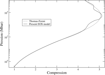
Figure 2: Standard Hugoniot curve for Fe ($\rho_{0}=$7.85 g/cm³) calculated from a model relying on Thomas-Fermi approximation and from our QSCF EOS model.

and $P_{xc}$ is the exchange-correlation pressure evaluated in the local density approximation [3]. The value of bound-electron pressure $P_{b}$ depends on the boundary conditions. This comes from the fact that the energy of an orbital depends on the value of the corresponding wavefunction and on its derivative at the boundary of the WS sphere. Table 1 represents the energies of the orbitals of iron (Fe, $Z$=26) obtained if the wavefunction cancels at the boundary (BC1), if the logarithmic derivative of the wavefunction cancels at the boundary (BC2) and if the wavefunction behaves like a decreasing exponential at the boundary (BC3). In this example, the mass density is equal to 34.83 g/cm³ and the temperature to 115.30 eV. Such conditions belong to the Hugoniot of Fe (see Fig. 2) calculated from the present QSCF model. The values of orbital energies displayed in table 1 show that the orbitals calculated with the three different boundary conditions will not be ionized for the same value of density. We chose to perform single-state calculations with boundary condition (BC3), since it allows the matching of wavefunctions with Bessel functions outside the WS sphere [4], where the potential is zero. Moreover, condition (BC3) is consistent with the fact that the bound-electron density vanishes at infinity. The internal energy is

$$E_{e} = \sum_{k}n_{k}\epsilon_{k}-\frac{1}{2}\int_{0}^{r_{ws}}n(r)\int_{0}^{r_{ws}}\frac{n(r^{\prime})}{|\vec{r}-\vec{r^{\prime}}|}d^{3}rd^{3}r^{\prime}$$ (11)

$$+E_{xc}-\int_{0}^{r_{ws}}n(r)V_{xc}(n(r))d^{3}r,$$

where $E_{xc}$ is the exchange-correlation internal energy and $n_{k}$ the population of state $k$ (either bound or free). The first term in (11) can be expressed by

$$\sum_{k}n_{k}\epsilon_{k}=\sum_{b}f_{l}(\epsilon_{b},\mu)\epsilon_{b}+E_{f,k}+E_{f,p}.$$ (12)

$E_{f,p}$ is the free-electron potential energy

$$E_{f,p}=\frac{\sqrt{2}(k_{B}T)^{3/2}}{\pi^{2}}\int_{0}^{r_{ws}}J_{1/2}\Big{(}-\bar{V}(r),\bar{\mu}-\bar{V}(r)\Big{)}\bar{V}(r)d^{3}r$$ (13)

and $E_{f,k}$ the free-electron kinetic energy

$$E_{f,k}=\frac{\sqrt{2}(k_{B}T)^{5/2}}{\pi^{2}}\int_{0}^{r_{ws}}J_{3/2}\Big{(}-\bar{V}(r),\bar{\mu}-\bar{V}(r)\Big{)}d^{3}r.$$ (14)

The ionic contribution to the EOS can be estimated in the ideal-gas approximation including non-ideality corrections to the thermal motion of ions. We used an approximation based on the calculation of the EOS of a one-component plasma (OCP) by the Monte Carlo method [6]. The ion contribution can be obtained using a formula based on the Virial theorem:

$$P_{i}(\rho,T)=\rho k_{B}T+\frac{\rho}{3}\Delta E_{i}(\rho,T),$$ (15)

where

$$\Delta E_{i}(\rho,T)=k_{B}T\;[\Gamma^{3/2}\sum_{i=1}^{4}\frac{a_{i}}{(b_{i}+\Gamma)^{i/2}}-a_{1}\Gamma]$$ (16)

and $E_{i}(\rho,T)=3k_{B}T/2+\Delta E_{i}(\rho,T)$ with $a_{1}=-0.895929$, $a_{2}=0.11340656$, $a_{3}=-0.90872827$, $a_{4}=0.11614773$, $b_{1}=4.666486$, $b_{2}=13.675411$, $b_{3}=1.8905603$ and $b_{4}=1.0277554$. $\Gamma$ is the plasma coupling parameter (ratio of ionic Coulomb interaction and thermal kinetic energy). In the present study, $\Gamma>1$.

The contributions $P_{e}(\rho,T)$ and $E_{e}(\rho,T)$ calculated from the QSCF model are not valid for $T\rightarrow 0$. Therefore, $P_{e}(\rho,0)$ and $E_{e}(\rho,0)$ must be substracted from total pressure and internal energy. They are replaced by $P_{c}(\rho)$ and $E_{c}(\rho)$, which constitute the cold curve. The total pressure reads now

$$P(\rho,T)=P_{e}(\rho,T)+P_{i}(\rho,T)-P_{e}(\rho,0)+P_{c}(\rho).$$ (17)

In our model, the cold curve is obtained either from Augmented Plane Waves (APW) [7] simulations, or using the Vinet [8] universal EOS. In many situations, Vinet EOS gives realistic results, and its accuracy is sufficient for most applications involving high pressure and high temperature situations.

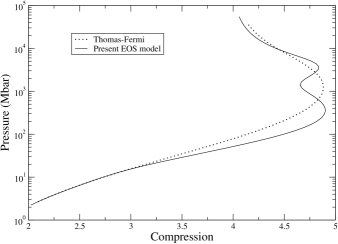
Figure 1: Standard Hugoniot curve for Al ($\rho_{0}=$2.70 g/cm³) calculated from a model relying on Thomas-Fermi approximation and from our QSCF EOS model.

Fig. 1 represents the principal Hugoniot curve for Al calculated from a model relying on Thomas-Fermi approximation and from the present QSCF model. Fig. 2 illustrates the same calculations in the case of Fe. One can check that the maximum compression is beyond the ideal-gas asymptote $\rho=4\rho_{0}$. The oscillations are a consequence of the competition between the release of energy stocked as internal energy within the shells and the free-electron pressure. When ionization begins, the energy of the shock is used mainly to depopulate the relevant shells and the material is very compressive. However, the pressure of free electrons in increasing number dominates again and the material becomes more difficult to compress. The two shoulders in the Hugoniot of Al are due to the successive ionization of L and K shells respectively. Similarly, the three shoulders in the Hugoniot of Fe are due to the successive ionization of M, L and K shells respectively. Table 2 illustrates the impact of the choice of the boundary conditions of the wavefunctions and of the calculation of the ionic part (perfect ideal gas (IG) with or without OCP corrections (15-16)) on the maximum compression rate. As for the eigen-energies (see table 1), (BC1) gives the highest value, (BC2) the lowest and (BC3) the intermediate one. The differences concerning the maximum compression rate appear to be less than 1 %. OCP corrections systematically increase the maximum compression rate.

3 Simple evaluation of maximum compression

The total energy can be written as the sum of kinetic and potential energies $E_{k}$ and $E_{p}$. Neglecting exchange-correlation contribution for a sake of simplicity, the virial theorem enables one to relate pressure, kinetic energy and potential energy:

$$3\frac{P}{\rho}=2E_{k}+E_{p}.$$ (18)

Using the Hugoniot relation (1), the compression rate $\eta=\rho/\rho_{0}$ for the standard Hugoniot ($P_{0}=0$, $\rho_{0}$ solid density and $T_{0}$=300 K) can be written

$$\eta=4+\frac{3}{1+2\frac{E_{k}-E_{k_{0}}}{E_{p}-E_{p_{0}}}}=4+\frac{3}{1+2\frac{\Delta E_{k}}{\Delta E_{p}}}.$$ (19)

At high compression, assuming that $E_{k}>>E_{k_{0}}$ and considering that all the electrons have been ionized and that all electrons have a kinetic energy equal to the Fermi energy, it is possible to write:

$$\Delta E_{k}=Z\frac{1}{2}(3\pi^{2}Z\rho\frac{N_{A}}{A})^{2/3}a_{0}^{2}.$$ (20)

At high compression, the excess potential energy can be estimated as the Coulomb interaction energy of two ionic spheres at close contact

$$\Delta E_{p}=\frac{1}{2}\frac{Z^{2}}{r_{ws}}\;\;\mbox{and}\;\;r_{ws}=\Big{[}\frac{3A}{4\pi N_{A}a_{0}^{3}}\Big{]}^{1/3}\rho^{-1/3},$$ (21)

where $r_{ws}$ is the WS radius defined by Eq. (3). Eqs. (20) and (21) are relevant for a strongly coupled gas of degenerate electrons. Therefore, putting Eqs. (20) and (21) in Eq. (19), the maximum compression rate $\eta_{m}$ obeys the following equation

$$\eta_{m}=4+\frac{3}{1+\gamma(\rho_{0},Z,A)\eta_{m}^{1/3}},$$ (22)

with

$$\gamma(\rho_{0},Z,A)=3\pi(2N_{A})^{1/3}a_{0}\Big{(}\frac{\rho_{0}}{ZA}\Big{)}^{1/3}.$$ (23)

Intermediate variable $X=\eta_{m}^{1/3}$ obeys the following fourth order equation

$$\gamma X^{4}+X^{3}-4\gamma X-7=0.$$ (24)

The solution is

$$\eta_{m}=\Big{[}\frac{-1+2\epsilon\gamma\sqrt{h(\gamma)}}{{4\gamma}}+\frac{1}{2}\sqrt{\frac{3}{4\gamma^{2}}-h(\gamma)+\epsilon\frac{32\gamma^{3}-1}{4\gamma^{3}\sqrt{h(\gamma)}}}\Big{]}^{3}$$ (25)

with $\epsilon=-1$ if $\gamma\leq 0.314980262473$ and $\epsilon=+1$ else,

$$h(\gamma)=\frac{1}{4\gamma^{2}}-\frac{2^{10/3}}{\Delta^{1/3}(\gamma)}+\frac{\Delta^{1/3}(\gamma)}{2^{1/3}\gamma},$$ (26)

and

$$\Delta(\gamma)=-7+16\gamma^{3}+\sqrt{49+1824\gamma^{3}+256\gamma^{6}}.$$ (27)

Neglecting cohesive and dissociation energies, and using fits for the total ionization energies, J.D. Johnson [9] has proposed an analytical formula for the maximum compression rate. Fig. 3 displays the maximum compression rate obtained from our analytical formula, from Ref. [9] and calculated with our QSCF model for Be, B, C, Na, Mg, Al, Fe and Cu. Exact values for those particular elements are indicated in table 3. It first confirms the fact that the maximum compression is always smaller than 7 [9], and strongly dependent on the density $\rho_{0}$. The most important point is that the maximum compression obtained with formula (25) is very close to the one obtained from our QSCF model. This means that Eq. (25), which does not rely on quantum mechanics, gives a good agreement with a quantum EOS model. At first sight, it seems difficult to decide in an unequivocal way which approach, between formula (25) and Ref. [9], is the most accurate. However, our estimate (25) does not rely on a particular form of the EOS and is fully analytical, since it does not require any data concerning the ionization energies, as in [9]. On the contrary to the formula proposed in [9], the maximum compression predicted by our analytical model is higher for Fe than for Al, which is consistent with the results presented in [10]. However, in [10] the authors notice that the maximum compression seems to increase with $Z$, even if they confess that they have no explanation for that. We believe this is only a global tendency, and Fig. 3 shows that the maximum compression, evaluated either from Ref. [9] or from Eq. (25), does not vary monotonically with atomic number $Z$.

4 Conclusion

A quantum equation-of-state model was presented. It consists in a self-consistent calculation of the electronic structure. Bound electrons are treated in the framework of quantum mechanics and bound-electron pressure is evaluated using the stress-tensor formula. Free electrons are described in the Thomas-Fermi approximation. Exchange-correlation effects at finite temperature are taken into account. The ionic part is described in the ideal-gas approximation with non-ideality corrections from the one-component plasma. It was shown that such a model is well suited for the computation of Hugoniot curves and exhibits oscillations due to the ionization of successive shells. A simple analytical estimate was proposed for the maximum compression attainable by a single shock, which is crucial for the diagnostic of high-pressure laser-induced shock waves. It relies on an expression for the increase of kinetic energy assuming degenerate electrons and the increase of potential energy is evaluated as Coulomb interation energy between hard spheres. Furthermore, the maximum compression obtained from this formula is in good agreement with the one calculated from our quantum EOS model.

Orbital	$\epsilon^{(BC1)}$ (a.u.)	$\epsilon^{(BC2)}$ (a.u.)	$\epsilon^{(BC3)}$ (a.u.)
1s	$-256.72931$	$-257.32658$	$-256.98981$
2s	$-29.891050$	$-30.363675$	$-30.094431$
2p	$-25.511960$	$-26.002778$	$-25.723564$
3s	$-2.3491653$	$-2.8962546$	$-2.5844217$
3p	$-1.0321504$	$-1.6990494$	$-1.3273471$

Table 1: Energies of orbitals of Fe at $\rho$=34.83 g/cm³ and T=115.30 eV for three boundary conditions: (BC1): the wavefunction is zero at the boundary, (BC2): the logarithmic derivative of the wavefunction is zero at the boundary and (BC3): the wavefunction behaves like a decreasing exponential at the boundary.

Boundary cond.	Ionic part	Max. compression rate
(BC1)	IG	$4.908$
(BC2)	IG	$4.891$
(BC3)	IG	$4.901$
(BC3)	IG+OCP corr.	$4.931$

Table 2: Impact of the boundary conditions of the bound-electron wavefunctions and of the treatment of ions on the maximum compression for Al.

Element	$Z$	$\eta_{m}[QSCF]$	$\eta_{m}[$Formula $(\ref{eta1})]$	$\eta_{m}[$Ref. $\cite[cite]{[\@@bibref{}{joh}{}{}]}]$
Beryllium	$4$	$4.56$	$4.70$	$4.31$
Boron	$5$	$4.61$	$4.73$	$4.36$
Carbon	$6$	$4.60$	$4.76$	$4.40$
Sodium	$11$	$5.07$	$5.23$	$5.63$
Magnesium	$12$	$5.20$	$5.13$	$5.27$
Aluminum	$13$	$4.90$	$5.07$	$5.06$
Iron	$26$	$5.12$	$5.15$	$5.02$
Copper	$29$	$5.14$	$5.18$	$5.04$

Table 3: Maximum compression rate for different elements calculated from our QSCF equation-of-state model, from our analytical formula (25) and from an estimate published in Ref. [9].

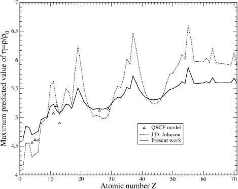
Figure 3: Maximum compression rate obtained from [9], from our model and compared to the maximum compression calculated from our QSCF model for Be, B, C, Na, Mg, Al, Fe and Cu.

References

- [1] R.P. Feynman, N. Metropolis, E. Teller, Phys. Rev. 75, 1561 (1949).
- [2] B.F. Rozsnyai, Phys. Rev. A 5, 231 (1972).
- [3] H. Iyetomi, S. Ichimaru, Phys. Rev. A 34, 433 (1986).
- [4] J.C. Pain, G. Dejonghe, T. Blenski, J. Quant. Spectrosc. Radiat. Transfer 99, 451 (2006).
- [5] J.C. Pain, G. Dejonghe, T. Blenski, J. Phys. A: Math. Gen. 39, 4659 (2006).
- [6] J.P. Hansen, Phys. Rev. A 8, 3096 (1973).
- [7] T.L. Loucks, Augmented Plane Wave Method: A Guide to Performing Electronic Structure Calculations (W.A. Benjamin, Inc., New York, 1967).
- [8] P. Vinet, J.H. Rose, J. Ferrante, J.R. Smith, J.Phys.: Condens. Matter 1, 1941 (1989).
- [9] J.D. Johnson, Phys. Rev. E 59, 3727 (1999).
- [10] B.F. Rozsnyai, J.R. Albritton, D.A. Young, V.N. Sonnad, D.A. Liberman, Phys. Lett. A 291, 226 (2001).