Electron operator at the edge of the 1/3 fractional quantum Hall liquid

Abstract

This study builds upon the work of Palacios and MacDonald (Phys. Rev. Lett. 76, 118 (1996)), wherein they identify the bosonic excitations of Wen’s approach for the edge of the 1/3 fractional quantum Hall state with certain operators introduced by Stone. Using a quantum Monte Carlo method, we extend to larger systems containing up to 40 electrons and obtain more accurate thermodynamic limits for various matrix elements for a short range interaction. The results are in agreement with those of Palacios and MacDonald for small systems, but offer further insight into the detailed approach to the thermodynamic limit. For the short range interaction, the results are consistent with the chiral Luttinger liquid predictions. We also study excitations using the Coulomb ground state for up to nine electrons to ascertain the effect of interactions on the results; in this case our tests of the chiral Luttinger liquid approach are inconclusive.

I Introduction

The low-energy excitations of an ordinary Landau Fermi liquid resemble electrons, and are perturbatively accessible from the free system. In recent years, there has been much interest in systems that do not conform to the Landau Fermi liquid paradigm. An example of a non-Landau Fermi liquid (NLFL) is the system of interacting fermions in one dimension, called a Tomonaga-Luttinger liquid, which is described by nonperturbative techniques such as bosonization [GiulianiVignale, ]. For Landau-Fermi liquids the electron spectral function has a sharp peak with a nonzero weight, called the quasiparticle renormalization factor. The quasiparticle renormalization factor vanishes for interacting electrons in one dimension.

For a FQHE state [Tsui, ], the excitations in the bulk are gapped, but arbirtarily low-energy excitations are available at the edge. The edge dynamics is one dimensional, and constitutes a realization of a chiral Luttinger liquid, which is a Luttinger liquid consisting of fermions moving only in one direction [WenIntJModPhy, ; Chang, ]. Here, only electrons at one edge of the FQHE system are considered; coupling with the oppositely moving electrons at the other edge is neglected, which is a good approximation for wide samples for which the two edges are spatially far separated. Wen has proposed an effective chiral Luttinger liquid (ECLL) model for the description of the FQHE edge [WenIntJModPhy, ], according to which the long distance properties at the edge are universal, described by a quantized exponent the value of which is determined by the quantized Hall resistance of the bulk FQHE state. The most direct probe of the properties of this liquid is tunneling of an external electron laterally into the edge of the FQHE system. Non-linear I-V characteristics have demonstrated NLFL behavior for the FQHE edge. The ECLL approach predicts an I-V behavior for the tunnel conductivity of the form $I\propto V^{\alpha}$, with a universal value for $\alpha$. In particular, for FQHE states at filling factors $\nu=n/(2pn+1)$, the effective approach predicts $\alpha=2p+1$. Experiments find a nontrivial value for $\alpha$ (i.e. $\alpha\neq 1$), but the observed $\alpha$ deviates from the predicted one [Grayson, ; Chang1, ; Chang2, ]. This discrepancy has motivated much work [Chang, ; Conti, ; MandalJain, ; ZulPalMacD, ; Lopez, ; Shytov, ], including the present paper.

The ECLL approach is built upon the idea of a one-to-one correspondence between the fermionic and bosonic Fock spaces in one dimension, and identifies a relationship between the operators of the two problems. In particular, the fermionic field operator $\hat{\psi}(x)$ is related to the bosonic field operator $\hat{\phi}(x)$ through the expression $\hat{\psi}(x)\sim\exp[-i\hat{\phi}(x)]$, which can be established rigorously for the ordinary one dimensional systems [GiulianiVignale, ]. A similar rigorous derivation has not been possible for the electron field operator at the edge of a FQHE system. Wen postulates that the electron operator at the edge of the $\nu=1/m$ FQHE system is given by

$$\hat{\psi}(x)\sim e^{-i\sqrt{m}\hat{\phi}(x)},$$ (1)

which has the virtue of satisfying the antisymmetry property when $m=2p+1$ is an odd integer [WenIntJModPhy, ]. This form leads to the quantized exponent for the I-V of the tunnel conductance. It is not known at the present what causes the discrepancy between the effective theory and experiment.

Our work is an outgrowth of the exact diagonalization studies of Palacios and MacDonald [PalaciosMacDonald, ] at $\nu=1/3$, the results of which were interpreted by the authors as confirming Wen’s ansatz. We now know, however, that the discrepancy is small at $\nu=1/3$ (the observed value of $\alpha\approx 2.7$ is close to the predicted $\alpha=3$), and the results of Ref. [PalaciosMacDonald, ] were not sufficiently accurate to capture such small deviations. We extend their calculations to larger systems, using a Monte Carlo method, to obtain more accurate thermodynamic extrapolations. Furthermore, Ref. [PalaciosMacDonald, ] assumed a short range interaction model; we also investigate to what extent the results are sensitive to the form of the interaction. Our results are consistent with the ECLL predictions for the short-range model, but inconclusive for the Coulomb interaction.

It should be stressed that the FQHE liquid itself provides a beautiful paradigm for a breakdown of the Landau-Fermi liquid concept. Here, strong interactions generate electron-vortex bound states called composite fermions, which are qualitatively distinct from, and perturbatively unrelated to, electrons [JainCFpaper, ; JainCFBook, ]. Composite fermions experience a greatly reduced effective magnetic field, and possess quantum numbers (for the local charge and braiding statistics) which are a fraction of the electron quantum numbers. The bulk properties of the composite fermion (CF) liquid have been investigated by a variety of means, and many experiments have directly verified the effective magnetic field, a clear indication of the NLFL nature of the state. The question of how an external electron, tunneling vertically in the CF liquid, couples to the system has been studied, and it has been predicted that it tunnels resonantly into an excited state, which is a bound state of several excited composite fermions, to produce a sharp peak in the electron spectral function [JainPet, ; Vignale, ]. The CF liquid therefore provides a different mechanism for the breakdown of the Landau-Fermi liquid concept: The electron renormalization factor remains nonzero, but lower energy states appear that are not described in terms of new quasiparticles.

The plan of the paper is as follows. Section II lists the connection between the bosonic approach and wave functions. The results are given in Sec. III, followed by conclusion in Sec. IV.

II Spectral weights

Following Palacios and MacDonald [PalaciosMacDonald, ] we test the validity of Eq. 1 by comparing the microscopically calculated spectral weights

$$C_{\{n_{l}\}}=\frac{\langle\{n_{l}\}|\hat{\psi}^{\dagger}(\theta)|0\rangle}{\langle 0|\hat{\psi}^{\dagger}(\theta)|0\rangle}$$ (2)

(where $\theta$ denotes the position in one dimension, wrapped into a circle via periodic boundary conditions) with the predictions of the ECLL approach. In the ECLL approach at filling factor $1/m$ [WenIntJModPhy, ], the vacuum state $|0\rangle$ contains no bosons and the various symbols have the following meaning:

$$\hat{\psi}^{\dagger}(\theta)=\sqrt{z}e^{i\sqrt{m}\hat{\phi}_{+}(\theta)}e^{-i\sqrt{m}\hat{\phi}_{-}(\theta)}$$ (3)

$$\hat{\phi}_{+}(\theta)=-i\sum_{l}\frac{1}{\sqrt{l}}a_{l}^{\dagger}e^{il\theta}$$ (4)

$$\hat{\phi}_{-}(\theta)=-i\sum_{l}\frac{1}{\sqrt{l}}a_{l}e^{-il\theta}$$ (5)

and

$$|\{n_{l}\}\rangle=\prod_{l=0}^{\infty}\frac{\left(a_{l}^{\dagger}\right)^{n_{l}}}{\sqrt{n_{l}!}}|0\rangle.$$ (6)

Here $a_{l}^{\dagger}$ and $a_{l}$ are creation and annihilation operators for a boson in the angular momentum $l$ state, with the total angular momentum given by

$$\Delta M=\sum_{l}l\,n_{l}.$$ (7)

By expanding $\exp[i\sqrt{m}\hat{\phi}_{+}(\theta)]$ and $\exp[-i\sqrt{m}\hat{\phi}_{-}(\theta)]$ in power series of products of $a_{l}$ and $a_{l}^{\dagger}$, it is straightforward to compute the analytical values for the spectral weights $C_{\{n_{l}\}}$. The square of the spectral weight $|C_{\{n_{l}\}}|^{2}$ is independent of the angular position parameter. The denominator in Eq. 2 eliminates the unknown normalization constant $\sqrt{z}$ in Eq. 3.

From the perspective of electrons, the vacuum state is the ground state of interacting electrons at $\nu=1/m$, and the field operator has the standard meaning of

$$\hat{\psi}^{\dagger}(\theta)=\sum_{l}\eta_{l}^{*}(\theta)c_{l}^{\dagger}\equiv\sum_{l}\psi_{l}^{\dagger}(\theta),$$ (8)

where $c_{l}^{\dagger}$ and $c_{l}$ are creation and annihilation operators for an electron in the angular momentum $l$ state, the wave function for which is $\eta_{l}$:

$$\eta_{l}(z)=\frac{z^{l}}{\sqrt{2\pi 2^{l}l!}}e^{-|z|^{2}/4},\;\;z=x-iy.$$ (9)

The denominator of Eq. 2 is interpreted as

$$\langle 0|\hat{\psi}^{\dagger}(\theta)|0\rangle=\langle\Psi_{0}^{N+1}|\hat{\psi}^{\dagger}(\theta)|\Psi_{0}^{N}\rangle$$ (10)

where $\Psi_{0}^{N}$ is the normalized ground state of $N$ interacting electrons at $\nu=1/m$. The numerator is interpreted as

$$\langle{\{n_{l}\}}|\hat{\psi}^{\dagger}(\theta)|0\rangle=\langle\Psi_{\{n_{l}\}}^{N+1}|\hat{\psi}_{L}^{\dagger}(\theta)|\Psi_{0}^{N}\rangle.$$ (11)

Here, we have,

$$\hat{\psi}_{L}^{\dagger}|\Psi_{0}^{N}\rangle=\mathcal{N}_{L}\mathcal{A}\left[z_{N+1}^{L}e^{-|z_{N+1}|^{2}/4}\Psi_{0}^{N}(z_{1},z_{2}\dots,z_{N})\right],$$ (12)

where ${\cal A}$ is the antisymmetrization operator and $\cal{N}_{L}$ is the normalization constant.

The wave function $\Psi_{\{n_{l}\}}^{N+1}$, the electronic counterpart of the bosonic state $|\{n_{l}\}\rangle$, represents an excited state that involves increasing the angular momentum of the $N$ particle ground state by $L$ units. It is not immediately obvious how to construct it for a general case. For the integral quantum Hall state at $\nu=1$, Stone showed [stone1, ; stone2, ; Oaknin, ] that it is obtained by multiplying the ($N+1$ particle) ground state by the factor $\prod_{l}S_{l}^{n_{l}}$, where $S_{l}$ are defined as:

$$S_{l}=\sum_{j=1}^{N}z_{j}^{l}.$$ (13)

The product increases the total angular momentum of the $N+1$ particle ground state by $\Delta M=\sum_{l}ln_{l}$. The composite-fermion analogy suggests the identification [PalaciosMacDonald, ]

$$|\Psi^{N+1}_{\{n_{l}\}}\rangle=\mathcal{N}_{n_{l}}\left(\prod_{l}(S_{l})^{n_{l}}\right)\Psi_{0}^{N}$$ (14)

at $\nu=1/m$, where $\mathcal{N}_{n_{l}}$ is the normalization constant. The angular momentum changes $L$ and $\Delta M$, defined relative to the $N$ and $N+1$ particle ground states, respectively, are related by

$$L=\Delta M+mN,$$ (15)

where the last term is the difference between the angular momenta of the ground states. We will assume the identification in Eq. 14 in what follows; further justification for it is given in the Appendix. In our calculations with exact diagonalization method, we will use that the second quantization representation for the operators $S_{l}$ is given by (apart from a constant factor)

$$S_{l}=\sum_{k=0}^{\infty}\sqrt{\frac{(k+l)!}{k!}}c_{k+l}^{\dagger}c_{k}.$$ (16)

III Results

III.1 Exact diagonalization: Short range interaction

Palacios and MacDonald [PalaciosMacDonald, ] computed the squared spectral weights $|C_{\{n_{l}\}}|^{2}$ defined in Eq. 2 by exact diagonalization for a short-range interaction model for which the Laughlin wave function [Laughlin, ] and the excited states in Eq. 14 are exact eigenstates. (This interaction takes a nonzero value for the $V_{1}$ pseudopotential [HaldanePseud, ] but sets all other pseudopotentials to zero.) They obtain results for systems containing up to eight electrons for $\Delta M=$1 to 4; from an extrapolation to the thermodynamic limit, they find approximate consistency with the predictions of the effective ECLL approach.

The results we obtained for $V_{1}$ interaction are shown in Table 1, and are identical to the results by Palacios and MacDonald [PalaciosMacDonald, ]. However, our extrapolation to thermodynamic limit differs slightly from theirs. The extrapolation assumes a leading finite size correction for $|C_{\{n_{l}\}}|^{2}$ proportional to $1/N$; this dependence has not been derived analytically, but matches the numerical data well for these particle numbers. The thermodynamic values are close to, but significantly different from, those predicted by the ECLL model.

III.2 “Exact” diagonalization: Coulomb interaction

A proper extension of the above results to the Coulomb interaction is not known. In the above, both the ground and excited states are exact eigenstates of the $V_{1}$ model. While the exact ground state for the Coulomb interaction can be obtained for small systems, no operators analogous to the $S_{l}$ of Eq. 13 are known that produce exact excited states. We use an approximate, “hybrid” approach, in which we take the exact Coulomb ground state, but use the same operators $S_{l}$ to create excited states. The above calculation can then be extended to the Coulomb interaction. The exact spectral weights with for angular momenta $\Delta M=1$ to 4 and particles $N=$4 to 9 are tabulated in Table 2. Again, there is a small, but significant, deviation from the ECLL results.

We mention here a technical point relating to the efficiency of the numerical calculation. The number of basis vectors increases rapidly with the number of particles. For example, for $\Delta M=0,N=8$ and $9$ and $10$, the number of basis vectors are 55,974, 403,016 and 2,977,866, respectively. During bosonic state creation and overlap calculation, the most time consuming step is searching for a given component from the ket vector $\psi^{\dagger}_{L}|\Psi_{0}^{N}\rangle$ and matching it with the corresponding bra vector component $\langle\Psi_{\{n_{l}\}}^{N+1}|$. We collect the fermionic states $|m_{1},m_{2},\dots,m_{N}\rangle$ into bins indexed by the smallest three angular momentum values $\{m_{1},m_{2},m_{3}\}$, which allows the search for a match to be restricted to a single bin. This reduces the computation time by a factor of 70, enabling computation of single boson states within 35 hours on our supercomputing cluster.

$\Delta M$	$\{n_{l}\}$	$N=4$	$N=5$	$N=6$	$N=7$	$N=8$	N$\rightarrow\infty$	ECLL
1	$\{1000\}$	2.6000	2.6667	2.7142	2.7500	2.778	2.9532	3
2	$\{2000\}$	3.6400	3.7778	3.8755	3.9531	4.012	4.3769	9/2
	$\{0100\}$	1.2585	1.2953	1.3224	1.3425	1.358	1.4562	3/2
3	$\{3000\}$	3.6400	3.7778	3.8775	3.9531	4.012	4.3777	9/2
	$\{1100\}$	3.6740	3.8133	3.9128	3.9860	4.041	4.4053	9/2
	$\{0010\}$	0.9356	0.9358	0.9390	0.9425	0.946	0.9543	1
4	$\{4000\}$	2.9120	2.9907	3.0466	3.088	3.121	3.3267	27/8
	$\{2100\}$	5.6503	5.8730	6.0247	6.131	6.209	6.7701	27/4
	$\{1010\}$	2.7489	2.7952	2.8284	2.852	2.869	2.9894	3
	$\{0200\}$	1.0184	1.0353	1.0484	1.058	1.064	1.1102	9/8
	$\{0001\}$	0.9044	0.8583	0.8302	0.8109	0.797	0.6881	3/4

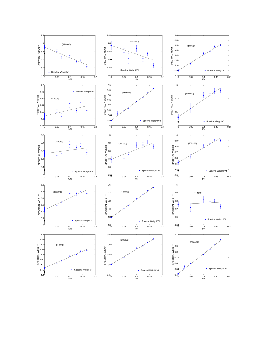
Figure 2: (Color online) Filled squares represent squared spectral weights $|C_{\{n_{l}\}}|^{2}$ obtained from Monte Carlo simulaton for $V_{1}$ interaction for $\Delta M=5,6$. The error bars indicate the statistical uncertainty in the Monte Carlo results. Thermodynamic extrapolation is also shown as a blue square on the vertical axis. Their numerical values are given in Table 3. ECLL predictions are shown as solid diamonds on the vertical axes.

Table 1: Squared spectral weights $|C_{\{n_{l}\}}|^{2}$ from exact diagonalization method for the short range model in which only the $V_{1}$ pseudopotential is nonzero. $N$ is the number of electrons in the study. For finite $N$, our numbers are identical to those in Ref. PalaciosMacDonald, , but our extrapolations to $N\rightarrow\infty$ are slightly different. ”(A linear extrapolation in $1/N$ is assumed for obtaining the thermodynamic limits in this table, in Tables II and III, and in Figs. 1 and 2 for the exact diagonalization results; the validity of this assumption is questioned by larger system Monte Carlo results shown in Fig. 1 for the short-range interaction.)

$\Delta M$	$\{n_{l}\}$	$N=4$	$N=5$	$N=6$	$N=7$	$N=8$	$N=9$	N$\rightarrow\infty$	ECLL
1	$\{1000\}$	2.6000	2.6670	2.7150	2.7514	2.7801	2.8031	2.9619	3
2	$\{2000\}$	3.6400	3.7783	3.8786	3.9553	4.0157	4.0644	4.3954	9/2
	$\{0100\}$	1.2871	1.3177	1.3504	1.3654	1.3744	1.3849	1.4658	3/2
3	$\{3000\}$	3.6400	3.7783	3.8786	3.9554	4.0157	4.0644	4.3954	9/2
	$\{1100\}$	3.7551	3.8768	3.9937	4.0522	4.0885	4.1265	4.4334	9/2
	$\{0010\}$	1.0029	0.9836	0.9925	0.9830	0.9780	0.9773	0.9588	1
4	$\{4000\}$	2.9120	2.9911	3.0475	3.0903	3.1233	3.1499	3.3365	27/8
	$\{2100\}$	5.7699	5.9657	6.1450	6.2311	6.2804	6.3315	6.8044	27/4
	$\{1010\}$	2.9313	2.9315	2.9843	2.9710	2.9636	2.9662	3.0087	3
	$\{0200\}$	1.0632	1.0700	1.0926	1.0935	1.0886	1.0898	1.1193	9/8
	$\{0001\}$	0.9676	0.9128	0.9095	0.8725	0.8420	0.8264	0.7259	3/4

Table 2: Squared spectral weights $|C_{\{n_{l}\}}|^{2}$ obtained from exact diagonalization method for the Coulomb interaction.

III.3 Monte Carlo simulation results

The exact diagonalization method has the drawback of being restricted to small numbers of particles. Fortunately with quantum Monte Carlo methods we can extend the results to much larger systems for the above-mentioned short-ranged $V_{1}$ interaction, for which all the wave functions in question are explicitly known. With the Monte Carlo calculation method we have obtained the spectral weights for up to 40 particles, for $\Delta M$ ranging from 1 to 6. The results are shown in Table 3 and Figs. 1 and 2.

III.4 Orthogonality

The ECLL approach also predicts orthogonality between states $|\Psi_{\{n_{l}\}}\rangle$ and $|\Psi_{\{n_{l}^{\prime}\}}\rangle$ for $\{n_{l}\}\neq\{n_{l}^{\prime}\}$. Such an orthogonality is not apparent from the wave function, and does not follow from any symmetry. We have numerically tested it for several cases; the results, summarized in Table 4, indicate that the overlap between different states rapidly diminishes with increasing number of particles. This also demonstrates that the states generated by the operators $S_{l}$ do not exactly represent free boson states for finite $N$, but are meaningful only in the thermodynamic limit.

IV Discussion and conclusions

The thermodynamic values of the spectral weights, obtained by assuming a linear fit as a function of $1/N$, lie within a few percent of the ECLL predictions (0.9 % to 18 % for single boson states; see Table 3), but the deviations between the two are often significant. However, deviations from linear fit are seen for large $N$. For example, for $\{1000\},\{0100\},\{3000\},\{1100\},\{0100\},\{0001\},\{010100\}$, $\{00001\},\{200100\},\{1000010\},\{01010\},\{002000\}$, $\{000001\}$ (Figs. 1 and 2), the actual fit is nonlinear, and tends toward the ECLL results with increasing $N$. A proper thermodynamic value is difficult to estimate accurately in many cases, partly because of the lack of analytic results regarding the $N$ dependence of $|C_{\{n_{l}\}}|^{2}$. However, the thermodynamic limits are in general agreement with the ECLL predictions. This is consistent with several previous studies [MandalJain, ; ZulPalMacD, ; Shytov, ] that confirm the validity of the ECLL model for the short range interaction.

With a partial inclusion of the Coulomb interaction, linear extrapolation of the results for up to nine particles again gives matrix elements that are close to the ECLL prediction but significantly different. The results are also in general quite different from those for short range interaction. Here, however, it is not possible to extend our study to larger systems. From our experience with the short range interaction, we cannot rule out deviation of the $|C_{\{n_{l}\}}|^{2}$ vs. $1/N$ plot from linearity for large $N$, and therefore consider our study as being inconclusive.

Our calculations essentially serve as a test of the identification of the operators $S_{l}$ with the boson operators $a_{l}$ for the short range interaction. This was first introduced by Palacios and MacDonald, and is further justified in the appendix, but not proven rigorously.

V Acknowledgement

One of us (S.J.) acknowledges Paul Lammert for many discussions and thanks Gun Sang Jeon and Csaba Töke for help with programming algorithm. We are grateful to A. H. MacDonald and J. J. Palacios for useful communications. The computational work was performed on the Lion-XO cluster of High Performance Computing Group, Pennsylvania State University. Partial support by the National Science Foundation under grant no. DMR-0240458 is acknowledged.

$\Delta M$	$\{n_{l}\}$	$|C_{\{n_{l}\}}|^{2}$	$|C^{ECLL}_{\{n_{l}\}}|^{2}$	% deviation
1	{1000}	2.9732(0.02)	3	0.89
2	{2000}	4.5136(0.02)	4.5	0.30
	{0100}	1.4760(0.01)	1.5	1.60
3	{3000}	4.4896(0.02)	4.5	0.23
	{1100}	4.4764(0.02)	4.5	0.52
	{0010}	0.9769(0.01)	1	2.31
4	{4000}	3.3833(0.03)	3.375	0.25
	{2100}	6.7928(0.05)	6.75	0.63
	{1010}	3.0005(0.02)	3	0.02
	{0200}	1.1273(0.01)	1.125	0.20
	{0001}	0.7210(0.01)	0.75	3.87
5	{50000}	2.0429(0.02)	2.025	0.88
	{31000}	6.9042(0.04)	6.75	2.28
	{20100}	4.5869(0.03)	4.5	1.93
	{10010}	2.2493(0.02)	2.25	0.03
	{01100}	1.5073(0.01)	1.5	0.49
	{00001}	0.5481(0.01)	0.6	8.65
6	{600000}	1.0303(0.01)	1.0125	1.76
	{410000}	5.2688(0.04)	5.0625	4.08
	{301000}	4.6980(0.04)	4.5	4.40
	{200100}	3.5203(0.03)	3.375	4.31
	{220000}	5.2251(0.04)	5.0625	3.21
	{100010}	1.7837(0.02)	1.8	0.91
	{111000}	4.7573(0.03)	4.5	5.72
	{010100}	1.1669(0.01)	1.125	3.72
	{002000}	0.5014(0.01)	0.5	0.28
	{000001}	0.4072(0.01)	0.5	18.56

Table 3: Monte Carlo simulation results for $V_{1}$ pseudopotential with 20 particles. Third column shows the thermodynamic extrapolation of squared spectral weight. The statistical errors are shown in parenthesis. ECLL predictions and deviation from ECLL predictions are shown in fourth and fifth columns, respectively.

$\Delta M$	$\{n_{l}\}$	$\{n_{l}^{\prime}\}$	$N=6$	$N=8$	$N=15$
2	$\{2000\}$	$\{0100\}$	6.90(0.1) $\times 10^{-3}$	4.3(0.12) $\times 10^{-3}$	1.3(0.06) $\times 10^{-3}$
3	$\{3000\}$	$\{1100\}$	2.1(0.05) $\times 10^{-2}$	1.2(0.03) $\times 10^{-2}$	4.0(0.06) $\times 10^{-3}$
	$\{3000\}$	$\{0010\}$	1.0(0.07) $\times 10^{-4}$	8.6(0.52) $\times 10^{-5}$	1.2(0.57) $\times 10^{-5}$
	$\{1100\}$	$\{0010\}$	4.3(0.03) $\times 10^{-2}$	2.7(0.10) $\times 10^{-2}$	7.7(0.24) $\times 10^{-3}$
4	$\{4000\}$	$\{2100\}$	4.0(0.05) $\times 10^{-2}$	2.5(0.03) $\times 10^{-2}$	8.1(0.20) $\times 10^{-3}$
	$\{4000\}$	$\{1010\}$	4.20(0.2) $\times 10^{-4}$	1.5(0.20) $\times 10^{-4}$	4.0(1.00) $\times 10^{-5}$
	$\{4000\}$	$\{0200\}$	1.0(0.05) $\times 10^{-4}$	5.0(0.30) $\times 10^{-5}$	5.5(1.40) $\times 10^{-6}$
	$\{4000\}$	$\{0001\}$	4.20(1.2) $\times 10^{-6}$	1.0(0.2.4) $\times 10^{-6}$	2.7(1.20) $\times 10^{-6}$
	$\{2100\}$	$\{1010\}$	8.1(0.05) $\times 10^{-2}$	5.0(0.04) $\times 10^{-2}$	1.6(0.01) $\times 10^{-2}$
	$\{2100\}$	$\{0200\}$	1.4(0.02) $\times 10^{-2}$	8.3(0.80) $\times 10^{-3}$	2.7(0.10) $\times 10^{-3}$
	$\{2100\}$	$\{0001\}$	1.8(0.05) $\times 10^{-3}$	6.8(0.30) $\times 10^{-4}$	8.0(1.10) $\times 10^{-5}$
	$\{1010\}$	$\{0200\}$	1.1(0.03) $\times 10^{-3}$	4.0(0.10) $\times 10^{-4}$	4.2(0.90) $\times 10^{-5}$
	$\{1010\}$	$\{0001\}$	8.8(0.05) $\times 10^{-2}$	5.3(0.04) $\times 10^{-2}$	1.6(0.02) $\times 10^{-2}$
	$\{0200\}$	$\{0001\}$	6.0(0.04) $\times 10^{-2}$	3.5(0.03) $\times 10^{-2}$	1.0(0.03) $\times 10^{-2}$

Table 4: Overlaps $|\langle\Psi_{\{n_{l}\}}|\Psi_{\{n_{l}^{\prime}\}}\rangle|^{2}$, where $\Psi_{\{n_{l}\}}$ is defined as in Eq. (14). Results are shown for $\Delta$M=1 to 4 for several values of $N$.

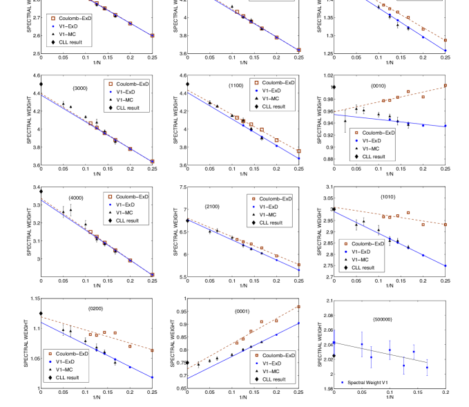
Figure 1: (Color online) Squared spectral weights $|C_{\{n_{l}\}}|^{2}$ obtained from several methods: exact diagonalization for short range interaction (labeled V1-ExD) and Coulomb interaction (Coulomb-ExD), and Monte Carlo evaluation for the short range interaction (V1-MC). The symbols are defined on the figures. The error bars indicate the statistical uncertainty in the Monte Carlo results. Results are shown for $\Delta M=1,2,3,4$ and 5. For $\Delta M=5$, $\{50000\}$ state we have only Monte Carlo results. The solid line and the dashed line are a linear fit for the exact diagonalization results for short range and Coulomb interactions, respectively. The chiral Luttinger liquid (CLL) predictions are marked by solid diamonds on the vertical axes.

Appendix A Bosonic operators

In the standard bosonization approach for one-dimensional Fermi systems, the density operators play the role of bosons. For the state at $\nu=1$, Stone observed [stone1, ] that the fermionic excitations at the edge can be mapped into linear combinations of products of symmetric polynomials $S_{l}$’s given in Eq. (13 ):

$$\Psi_{\{\lambda_{k}\}}^{N} = \left|\begin{array}[]{rrrr}z_{1}^{\lambda_{1}+N-1}&z_{1}^{\lambda_{2}+N-2}&\cdots&z_{1}^{\lambda_{N}}\\ z_{2}^{\lambda_{1}+N-1}&z_{2}^{\lambda_{2}+N-2}&\cdots&z_{2}^{\lambda_{N}}\\ \vdots&\vdots&\vdots&\vdots\\ z_{N}^{\lambda_{1}+N-1}&z_{N}^{\lambda_{2}+N-2}&\cdots&z_{N}^{\lambda_{N}}\\ \end{array}\right|e^{-\sum_{i=1}^{N}|z|_{i}^{2}/4}$$ (21)

$$= \sum_{\{n_{l}\}}C^{\{\lambda_{k}\}}_{\{n_{l}\}}\prod_{l}S_{l}^{n_{l}}\Phi_{\{0\}}^{N},$$ (22)

where $\Phi^{N}_{\{0\}}$ is the ground state at $\nu=1$, $C^{\{\lambda_{k}\}}_{\{n_{l}\}}$’s are the expansion coefficients (cf. Eq 4.12 in [stone1, ]), $\lambda_{1}\geq\lambda_{2}\geq\cdots\lambda_{N}$, and $\sum_{k}\lambda_{k}=\sum_{l}ln_{l}=\Delta M$ is the total angular momentum of the excited state, measured relative to the ground state. The symmetric polynomial $S_{l}$ is identified with bosonic operator $a^{\dagger}_{l}$ at angular momentum $l$. We now ask under what conditions the operators $S_{l}$ satisfy the canonical commutation relations. For this purpose, we use the form given in Eq.(16).

The commutation relation $[S_{k},S_{l}]=0$, where $k$ and $l$ denote angular momentum quantum numbers, follows from the fact that the $S$’s can be expressed as polynomials, and can also be verified straightforwardly using the operator form of $S$ in Eq. (16). Demonstration of

$$[S_{k},S_{l}^{\dagger}]\propto\delta_{kl}$$ (23)

is more tricky. An explicit evaluation gives

$$[S_{k},S_{l}^{\dagger}] = \sum_{m}\sqrt{\frac{(m+k)!(m+l)!}{m!^{2}}}c_{m+k}^{\dagger}c_{l+m}$$ (24)

$$-\sum_{m}\sqrt{\frac{(m+k)!^{2}}{m!(m+k-l)!}}c_{m+k-l}^{\dagger}c_{m},$$

the right hand side of which, in general, does not vanish for $k\neq l$.

To proceed further, we assume the idealized occupation number for the ground state $\Omega$:

$$\langle\Omega|c_{k}^{\dagger}c_{k}|\Omega\rangle=\left\{\begin{array}[]{ll}\nu&\textrm{ if $k\leq M$}\\ 0&\textrm{otherwise ,}\end{array}\right.$$

where $M$ is the angular momentum of the outermost occupied orbital. This is surely correct for $k<<M$, but only approximate near the edge. We further assume that the effect of the operators $S_{l}$ is confined to the edge; this is manifestly correct for $\nu=1$, but not obvious for the FQHE state $\nu=1/m$.

We first consider $k=l$. Defining normal ordering of operators in the usual manner (i.e., by subtracting the ground state expectation value), we get

$$[S_{k},S_{k}^{\dagger}] = \sum_{m=0}^{\infty}\frac{(m+k)!}{m!}\Big{(}:c_{m+k}^{\dagger}c_{m+k}:-:c_{m}^{\dagger}c_{m}:$$ (25)

$$+ \langle\Omega|c_{k+m}^{\dagger}c_{k+m}|\Omega\rangle-\langle\Omega|c_{k}^{\dagger}c_{k}|\Omega\rangle\Big{)}.$$

The dominant contribution comes from the last two terms on the right hand side. (When only terms near the edge contribute to the commutator, then for $m\approx M$, the factorial term varies as $M^{k}$, and the normal ordered terms cancel to the lowest order.) This gives

$$[S_{k},S_{k}^{\dagger}] \approx \sum_{m=0}^{\infty}\frac{(m+k)!}{m!}\left(\langle\Omega|c_{k+m}^{\dagger}c_{k+m}|\Omega\rangle-\langle\Omega|c_{k}^{\dagger}c_{k}|\Omega\rangle\right)$$ (26)

$$= \sum_{m=M-k+1}^{M}\frac{(m+k)!}{m!}\left(0-\nu\right)$$

$$\approx -\nu kM^{k}.$$

The canonical bosonic relations are obtained by defining

$$a_{k}^{\dagger}=\frac{1}{\sqrt{\nu kM^{k}}}S_{k},\;\;k>0.$$ (27)

Next we consider the case when $k\neq l$, assuming $k>l$ and $N\gg\{k,l\}$ (since only excitations near the edge are significant). The commutator can be expressed as

$$[S_{k},S_{l}^{\dagger}] \approx \sum_{m}\Bigg{(}\sqrt{\frac{(m+k-l)!m!}{(m-l)!^{2}}}$$ (28)

$$- \sqrt{\frac{(m+k)!^{2}}{m!(m+k-l)!}}\Bigg{)}:c_{m+k-l}^{\dagger}c_{m}:$$

We have used above that the vacuum expectation values of all combinations on the right hand side vanish due to angular momentum conservation. Only terms for which $m\approx M$ are significant in the summation. A little algebra using the asymptotic expansion

$$n^{q-p}\frac{\Gamma(n+p)}{\Gamma(n+q)} = 1+\frac{(p-q)(p+q-1)}{2n}$$ (29)

$$+\frac{1}{12n^{2}}\displaystyle{p-q\choose 2}\left(3(p+q-1)^{2}-p+q-1\right)$$

$$+\cdots$$

shows that the commutator vanishes to leading order, producing

$$[S_{k},S_{l}^{\dagger}]\approx\sum_{m\approx M}\sqrt{m^{k+l}}\mathcal{O}(1/m^{2})c_{m+k-l}^{\dagger}c_{m}.$$ (30)

For the bosonic operators defined in Eq. (27), this implies

$$[a_{k}^{\dagger},a_{l}]\approx\sum_{m\approx M}\sqrt{\left(\frac{m}{M}\right)^{k+l}}\mathcal{O}(1/m^{2})c_{m+k-l}^{\dagger}c_{m}\to 0,$$ (31)

thus completing the relationship between $S_{l}$ and $b_{l}^{\dagger}$. We note that these considerations are valid for arbitrary $\nu$, but assume that the effect of the operators $S_{l}$ is confined to the edge.

References

- (1) For review, see: G.D. Mahan, Many Particle Physics, third edition (Plenum, New York, 2000); G. F.Giuliani and G. Vignale, Quantum Theory of Electron Liquid, Cambridge University Press,(2005); J. von Delft and H. Schoeller, Ann. Phys. (Leipzig) 7, 225 (1998).
- (2) D. C. Tsui, H. L. Stormer, and A. C. Gossard, Phys. Rev. Lett. 48, 1559 (1982).
- (3) X.G.Wen, Int. J. Mod. Phys. B, 6, 1711 (1993).
- (4) A. M. Chang, Rev. Mod. Phys, 75, 1449 (2003).
- (5) M. Grayson , D.C. Tsui, L.N. Pfeiffer, K.W. West, and A. M. Chang , Phys. Rev. Lett. 80 , 1062 (1998).
- (6) A. M. Chang, L.N. Pfeiffer, and K.W. West, Phys. Rev. Lett. 77, 2538 (1996).
- (7) A. M. Chang, M.K. Wu, C.C. Chi, L.N. Pfeiffer, and K.W. West, Phys. Rev. Lett. 86, 143 (2001).
- (8) S. Conti and G. Vignale, Phys. Rev. B 54, R14309 (1996).
- (9) S. S. Mandal and J. K. Jain, Solid State Communication 118, 503 (2001); Phys. Rev. Lett. 89 , 096801 (2002).
- (10) U. Zülicke, J.J. Palacios, and A.H. MacDonald, Phys. Rev. B 67, 045303 (2003); X. Wan, F. Evers and E.H. Rezayi, Phys. Rev. Lett. 94, 166804 (2005).
- (11) A. Lopez and E. Fradklin, Phys. Rev. B 59, 15323 (1999).
- (12) A.V. Shytov, L.S. Levitov, and B. I. Halperin, Phys. Rev. Lett. 80, 141 (1998).
- (13) J.J Palacios and A.H. MacDonald , Phys. Rev. Lett. 76, 118 (1996)
- (14) J.K. Jain, Phys. Rev. Lett. 63 199 (1989).
- (15) J. K. Jain, Composite Fermions (Cambridge University Press, 2007).
- (16) J.K. Jain, M.R. Peterson, Phys. Rev. Lett, 94, 186808 (2005).
- (17) G. Vignale, Phys. Rev. B 73, 073306 (2006).
- (18) M. Stone, Phys.. Rev. B 42, 8399(1990).
- (19) M. Stone, H. W. Wyld, and R. L. Schult, Phys. Rev. B 45, 14156 (1992).
- (20) J. H. Oaknin, L. Mart n-Moreno, J. J. Palacios, and C. Tejedor, Phys. Rev. Lett. 74, 5120 (1995).
- (21) R.B. Laughlin, Phys. Rev. Lett. 50, 1395 (1983).
- (22) F.D.M. Haldane, in Quantum Hall Effect, edited by R. Prange and S.M. Girvin (Springer Verlag, New York, 1987).