Detecting spatial patterns with the cumulant function.
Part I: The theory

Zusammenfassung

In climate studies, detecting spatial patterns that largely deviate from the sample mean still remains a statistical challenge. Although a Principal Component Analysis (PCA), or equivalently a Empirical Orthogonal Functions (EOF) decomposition, is often applied on this purpose, it can only provide meaningful results if the underlying multivariate distribution is Gaussian. Indeed, PCA is based on optimizing second order moments quantities and the covariance matrix can only capture the full dependence structure for multivariate Gaussian vectors. Whenever the application at hand can not satisfy this normality hypothesis (e.g. precipitation data), alternatives and/or improvements to PCA have to be developed and studied.

To go beyond this second order statistics constraint that limits the applicability of the PCA, we take advantage of the cumulant function that can produce higher order moments information. This cumulant function, well-known in the statistical literature, allows us to propose a new, simple and fast procedure to identify spatial patterns for non-Gaussian data. Our algorithm consists in maximizing the cumulant function. To illustrate our approach, its implementation for which explicit computations are obtained is performed on three family of of multivariate random vectors. In addition, we show that our algorithm corresponds to selecting the directions along which projected data display the largest spread over the marginal probability density tails.

1 Introduction

In geosciences, Principal Component Analysis (PCA) has been an essential and powerful tool at detecting spatial structures amongst time series recorded at different locations. PCA aims at building a decorrelated representation of the data and it finds the spatial patterns responsible for the largest proportion of variability Rencher, (1998). PCA can also be viewed as a dimensionality reduction technique that extracts the most relevant components of data, i.e. the ones that maximize the variances. Hence, second order moments are the foundation of PCA. But relying exclusively on second moments implies that PCA is only optimal when applied to multivariate Gaussian vectors. Although rarely stated and even more rarely checked, this underlined normality assumption is not always satisfied in practice.

Recently, different approaches have been tested to extend the applicability of PCA in geosciences. In particular, NonLinear PCA (NLPCA) has been applied to several geophysical datasets (e.g., Hsieh,, 2004; Monahan et al.,, 2001). In the NLPCA algorithm, data are considered as the input of an auto-associative neural network with five layers, with a bottleneck in the third layer Kramer, (1991). Through the minimization of a cost function, the output is forced to be as close as possible to the input, and the bottleneck layer is a low dimensional representation of the input. Since this neural network is nonlinear, NLPCA goes automatically beyond correlations. However, NLPCA suffers the intrinsic limitations of multilayered networks (e.g., Christiansen,, 2005; Malthouse,, 1998): it is computationally expensive and does not always converge to a global solution. To overcome these difficulties, we pursue a less ambitious aim: instead of trying to find decompositions that can explain the entire body of data with respect to a criterion, we focus on the part of data responsible for large anomalous behaviors.

In contrast to PCA, our approach tends to give maximal weight to data points which largely deviate from the mean, and to find the corresponding representative spatial patterns, i.e. the directions along which such points are prominently distributed. The key element in our procedure is the expansion of the cumulant function that can provide information beyond the first two moments. By maximizing the cumulant function (Kenney and Keeping,, 1951) over growing hyperspheres in the data space, a set of components can be derived. We first apply our procedure to three types of multivariate random vectors (Normal, Skew-Normal, Gamma). Then we demonstrate in the general case that if a direction exists for which the marginal probability density of projected data display a larger tail than in all other directions, then our procedure is able to select that direction.

When finding the first component, we show that PCA is a special case of our approach whenever the Gaussian assumption is satisfied. Besides the Gaussian case we show that, for any probability density, the solution derived from the centered cumulant function can be transformed to the first principal component by decreasing the radius of the hypersphere. Other principal components could be found as well, by a generalization of the proposed method. Our method is computationally cheap, and the solutions are found in the form of unit (normalized) vectors, as in the case of PCA, allowing a unidimensional projection with an easy geometrical interpretation.

In summary, this paper focuses on the problem of characterizing spatial patterns associated to large anomalies, i.e. large deviations from the sample mean, when the data set under study cannot be assumed to be normally distributed.

2 Maximizing the cumulant function

In the univariate case, the cumulant function of the random variable $X$ with finite moments is defined as the following scalar function

$$\log\Big{\{}\mathbb{E}\big{[}\exp(sX)\big{]}\Big{\}}=\sum_{n=1}^{\infty}\kappa_{n}{s^{n}\over n!},$$

where $s\in\mathbb{R}$, $\mathbb{E}(.)$ represents the mean function and the scalar $\kappa_{n}$ corresponds to the $n^{th}$ cumulant of $X$.

The first two cumulants $\kappa_{1}$ and $\kappa_{2}$ are simply the mean and the variance of $X$, respectively. The third and fourth cumulants are classically called the skewness and the kurtosis parameters. Concerning the existence of cumulants, we assume in this paper that all the cumulant coefficients are finite and that the cumulant function is always well defined. The cumulant function and its coefficients have many interesting properties. For example, if $X$ and $Y$ are two independent random variables then the $n^{th}$ cumulant of the sum $X+Y$ is equal to the sum of the $n^{th}$ cumulant of $X$ and the $n^{th}$ cumulant of $Y$ for any integers $n$. If $X$ follows a Gaussian distribution, then all but the first two cumulants are equal to zero. In a multivariate framework, the cumulant function of the random vector ${\bf X}=(X_{1},\dots,X_{m})^{t}$ is simply defined as

$$\log\Big{\{}\mathbb{E}\big{[}\exp({\bf s}^{t}{\bf X})\big{]}\Big{\}}\mbox{, for all ${\mathbf{s}}^{t}=(s_{1},\dots,s_{m})\in\mathbb{R}^{m}$.}$$ (1)

As in the univariate case, the linear and Gaussian properties associated to the cumulant function defined by (1) still hold, but the cumulant coefficients formulas are more cumbersome to write down in a multivariate framework. For more information about cumulants, we refer the reader to Kenney and Keeping, (1951).

To identify possible favorite projection directions with respect to the multivariate cumulant function, we first rewrite the vector ${\mathbf{s}}=(s_{1},\dots,s_{m})^{t}$ in (1) as the product ${\mathbf{s}}=|{\mathbf{s}}|\times\mbox{\boldmath$\theta$}$, where $|{\mathbf{s}}|^{2}=\sum s_{i}^{2}$, the scalar $|{\mathbf{s}}|$ represents the norm (“radius”) of ${\mathbf{s}}$ and $\theta$ is the unit “angular/direction”vector defined as $\theta_{i}=s_{i}/|{\mathbf{s}}|$ (note that $\mbox{\boldmath$\theta$}^{t}\mbox{\boldmath$\theta$}=1$). Secondly, the cumulant function for our vector ${\bf X}=(X_{1},\dots,X_{m})^{t}$ projected along the direction vector $\theta$ is introduced as

$$G_{|{\mathbf{s}}|}(\mbox{\boldmath$\theta$}) = \log\Big{\{}\mathbb{E}\big{[}\exp(|{\mathbf{s}}|\;{\mbox{\boldmath$\theta$}}^{t}{\bf X})\big{]}\Big{\}},$$ (2)

$$= \sum_{n=1}^{\infty}k_{n}(\mbox{\boldmath$\theta$})\frac{|{\mathbf{s}}|^{n}}{n!}.$$

Our algorithmic strategy is to maximize the cumulant function at fixed non-small $|{\mathbf{s}}|$ with respect to the angular component $\theta$ that varies over an unit hypersphere. Practically, we have to find the optimal $\mbox{\boldmath$\theta$}_{s}$ directions defined by

$$\mbox{\boldmath$\theta$}_{s}=\mbox{argmax}\left[G_{|{\mathbf{s}}|}(\mbox{\boldmath$\theta$})\mbox{ such that }{\mbox{\boldmath$\theta$}^{t}\mbox{\boldmath$\theta$}=1}\right],\mbox{ for any $|{\mathbf{s}}|$.}$$ (3)

If the radius $|{\mathbf{s}}|$ is small enough, and the mean $k_{1}$ is zero, the variance $k_{2}(\mbox{\boldmath$\theta$})$ dominates the centered cumulant function and the contributions of other cumulants can be neglected. In this situation, finding the first PCA component can be viewed as a special case of this optimization procedure, because maximizing the cumulant function for small $|{\mathbf{s}}|$ is equivalent to maximize the variance. As the value of $|{\mathbf{s}}|$ grows, higher and higher order cumulants become more dominant. Our main goal is to find $\mbox{\boldmath$\theta$}_{s}$ in (3) for the largest admissible $|{\mathbf{s}}|$ and study their properties. We will call the solutions of such an optimization scheme the Maxima of the Cumulant Function (MCF) directions.

We anticipate that, since the scalar product ${\bf\theta}^{t}{\bf X}$ is invariant under orthogonal transformations, the cumulant function is invariant as well. Given that the unit hypersphere is also invariant, our algorithm is symmetric respect to orthogonal transformations. For instance, if data vectors are rotated by a given angle, the solutions of the algorithm, in terms of $\theta$, are rotated by the same amount. This symmetry implies that if the probability density is isotropic, then the cumulant function is isotropic as well, and no relative maxima of $G$ exist on the unit hypersphere. In that case no directions are selected: for a rotationally symmetric distribution there is indeed no preferred direction along which anomalies are prominent, they are distributed uniformly over all angles.

To illustrate our optimization procedure we derive explicit cumulant maximization schemes for three special cases of multivariate family distributions, see Section 3. For assessing the outputs of our algorithm when applied to real data, we refer the reader to the second part of this paper Bernacchia et al., (2007)).

3 Theoretical examples

To study the properties of the maximization method developed in Section 2, three examples of distribution functions are considered in this paper. We choose these three families because explicit results can be derived and they have been classically used in the statistical modeling of temperatures and precipitation data.

Without loss of generality, some relevant matrices are diagonal thereafter. However, since the solutions are invariant respect to orthogonal transformations, they may be rotated along with the corresponding coordinate change. Analytical calculations are performed for the general multivariate case, while figures are given for the bivariate case.

3.1 Multivariate Gaussian vectors

Suppose that the data at hand can be appropriately fitted by a multivariate Gaussian vector. We assume that the observations have been centered (zero) mean and we denote the covariance matrix as $\Sigma$. The cumulant function of the centered Gaussian vector (e.g., Kenney and Keeping,, 1951) is equal to

$$\log\Big{\{}\mathbb{E}\big{[}\exp({\bf s}^{t}{\bf X})\big{]}\Big{\}}={1\over 2}{\bf s}^{t}\Sigma{\bf s}.$$

Hence, it is easy to show that all cumulants but the second are equal to zero. The decomposition in Equation (2), ${\mathbf{s}}=|{\mathbf{s}}|\times\mbox{\boldmath$\theta$}$, implies that the cumulant function becomes

$$G_{|{\mathbf{s}}|}(\mbox{\boldmath$\theta$})=\frac{|{\mathbf{s}}|^{2}}{2}k_{2}(\mbox{\boldmath$\theta$})=\frac{|{\mathbf{s}}|^{2}}{2}\;\mbox{\boldmath$\theta$}^{t}{\bf\Sigma}\mbox{\boldmath$\theta$}$$

Our optimization problem is to maximize $G_{|{\mathbf{s}}|}(\mbox{\boldmath$\theta$})$ under the constraint $\mbox{\boldmath$\theta$}^{t}\mbox{\boldmath$\theta$}=1$. To find the optimal $\mbox{\boldmath$\theta$}_{s}$ defined by (3), we introduce a function to be maximized, constrained by the Lagrange multiplier $\lambda$, as

$$\frac{|{\mathbf{s}}|^{2}}{2}\;\mbox{\boldmath$\theta$}^{t}{\bf\Sigma}\mbox{\boldmath$\theta$}-\lambda(\mbox{\boldmath$\theta$}^{t}\mbox{\boldmath$\theta$}-1).$$

Setting the gradient with respect to $\theta$ to zero gives

$$2\frac{|{\mathbf{s}}|^{2}}{2}{\bf\Sigma}\mbox{\boldmath$\theta$}-2\lambda\mbox{\boldmath$\theta$}=0.$$ (4)

Let $\lambda_{\Sigma}$ be the largest eigenvalue of the covariance matrix ${\bf\Sigma}$ and $\mbox{\boldmath$\theta$}_{\Sigma}$ its associated eigenvector. Introducing $\lambda_{s}={|{\mathbf{s}}|^{2}\over 2}\lambda_{\Sigma}$, we can write ${|{\mathbf{s}}|^{2}\over 2}{\bf\Sigma}\mbox{\boldmath$\theta$}_{\Sigma}=\lambda_{s}\mbox{\boldmath$\theta$}_{\Sigma}$. Consequently, $\mbox{\boldmath$\theta$}_{\Sigma}$ is the solution of (4). Note that $\mbox{\boldmath$\theta$}_{\Sigma}$ depends on $\Sigma$ but not on $|\bf s|$. The optimal direction, for the Gaussian case, is $\mbox{\boldmath$\theta$}_{s}=\mbox{\boldmath$\theta$}_{\Sigma}$, and it corresponds to the classical first principal component.

To illustrate this result, a bivariate vector of the normal distribution is presented in Figure 1 (in which a contour plot is drawn in logarithmic scale). The matrix $\bf\Sigma$ is assumed to be diagonal, with entries 1.2 and 0.5143.

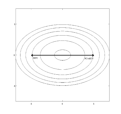
Abbildung 1: Isoprobability contours of the multivariate Gaussian distribution, with zero mean and variances $1.2$ and $0.5143$ (entries of the diagonal covariance matrix). The first principal component is shown (PC1), together with the two (opposite) maxima of the cumulant function (MCF1 and MCF2). All vectors are in arbitrary scale. The maxima of cumulant function are parallel to the first principal component, all pointing towards the large anomalies, in terms of high probability (at fixed vector norm). Probability contours are $10^{-1}$,$10^{-3}$,$10^{-5}\ldots 10^{-11}$

The first principal component (PC1), corresponding to the eigenvalue 1.2 is horizontal, while the second principal component, corresponding to the eigenvalue 0.5143 is vertical, and is not displayed. The two maxima of the cumulant function (MCF1 and MCF2) are just the positive and negative part of PC1. Indeed, both $\mbox{\boldmath$\theta$}_{\Sigma}$ and $-\mbox{\boldmath$\theta$}_{\Sigma}$ are solutions of (4). While this is always true for PCA, the maxima of the cumulant function may in general neither be parallel nor orthogonal.

PC1 is indeed the direction along which large anomalies are ditributed in the Gaussian case. In order to derive PC2 and other higher principal components from the cumulant function, one would have to determine not only its maxima, but also its minima and saddle points.

3.2 Multivariate Skew-Normal vectors

To introduce skewness to the Gaussian density, while keeping some of valuable properties of the normal distribution, Azzalini and his co-authors (e.g Azzalini and Dalla Valle,, 1996; Azzalini and Capitanio,, 1999; Gonzalez-Farias et al.,, 2004) have extended the normal density to a larger class called the Skew-Normal (SN) density, that is defined as

$$f(\mathbf{x})=2\phi_{\Sigma}(\mathbf{x})\Phi(\mbox{\boldmath$\alpha$}^{t}\mathbf{x})$$ (5)

where $\phi$ is a multivariate Normal probability density function with zero mean and covariance matrix $\Sigma$, and $\Phi$ is the cumulative density function of an univariate Gaussian random variable with zero mean and unit variance. The vector $\alpha$ corresponds to the degree of skewness. When $\alpha=0$, there is no skewness, and the SN distribution reduces to the Gaussian case. From (5), it is possible to derive the cumulant function (e.g Azzalini and Dalla Valle,, 1996) of a SN vector

$$\log\Big{\{}\mathbb{E}\big{[}\exp({\bf s}^{t}{\bf X})\big{]}\Big{\}}={1\over 2}{\bf s}^{t}\Sigma{\bf s}+\log\left(2\Phi({\scriptstyle\sqrt{\frac{\pi}{2}}}\mbox{\boldmath$\mu$}^{t}{\bf s})\right).$$

where $\mu$ represents the mean vector, and is equal to

$$\mbox{\boldmath$\mu$}=\frac{\Sigma\mbox{\boldmath$\alpha$}}{\sqrt{\frac{\pi}{2}(1+\mbox{\boldmath$\alpha$}^{t}\Sigma\mbox{\boldmath$\alpha$})}}.$$

Note that the covariance matrix of the SN distribution is not $\Sigma$ but $\Sigma-\mbox{\boldmath$\mu$}\mbox{\boldmath$\mu$}^{t}$ (Azzalini and Capitanio,, 1999).

A bivariate example of the SN distribution is presented in Figure 2, in which a contour plot is drawn in logarithmic scale. The matrix $\Sigma$ is chosen to be diagonal with entries $1.2$ and $0.5143$. The skewness vector $\alpha$ is taken to be equal to $(4.365,-1.455)$. The distribution in Figure 2 has been centered such that the mean vector is zero. In the bivariate example, $\mu$ is $(0.8367,-0.1195)$.

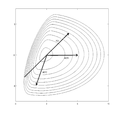
Abbildung 2: Isoprobability contours of the multivariate Skew-Normal distribution, with parameters $\alpha=(4.365,-1.455)$ and the matrix $\Sigma$ is chosen to be diagonal with entries $1.2$ and $0.5143$. The first principal component is shown (PC1), together with the two maxima of the cumulant function (MCF1 and MCF2). All vectors are in arbitrary scale. In this case, the two maxima of the cumulant function are not related to the first principal component, and point towards the (local) large anomalies, in terms of high probability (at fixed, and large, vector norm). Probability contours are $10^{-1}$,$10^{-3}$,$10^{-5}\ldots 10^{-19}$

From the SN cumulant function (Azzalini and Capitanio,, 1999), we can write the cumulant function of the centered vector $\mbox{\boldmath$\theta$}^{t}({\bf X}-\mbox{\boldmath$\mu$}$) as

$$G_{|{\mathbf{s}}|}(\mbox{\boldmath$\theta$})=-|{\mathbf{s}}|\mbox{\boldmath$\mu$}^{t}\mbox{\boldmath$\theta$}+{|{\mathbf{s}}|^{2}\over 2}\mbox{\boldmath$\theta$}^{t}\Sigma\mbox{\boldmath$\theta$}+\mbox{log}\Big{[}2\Phi({\scriptstyle\sqrt{\frac{\pi}{2}}}|{\mathbf{s}}|\mbox{\boldmath$\mu$}^{t}\mbox{\boldmath$\theta$})\Big{]}$$ (6)

While it is not possible to find explicit solutions of the maximization problem defined by (3) for (6), one can provide valuable approximated solutions for both small and large $|{\mathbf{s}}|$. In the former case, the following two Taylor expansions are the key elements to derive our results

$$\mbox{log}(1+s)=1+s-\frac{s^{2}}{2}+o(s^{3})\mbox{ and }$$ (7)

$$1+\mbox{erf}(s)=1+\;\frac{2s}{\sqrt{\pi}}+o(s^{3})$$ (8)

where erf corresponds to the error function defined by

$$2\Phi(s)=1+\mbox{erf}\Big{(}\frac{s}{\sqrt{2}}\Big{)}.$$

Then we can write the following approximation

$$\mbox{log}\Big{[}2\Phi({\scriptstyle\sqrt{\frac{\pi}{2}}}|{\mathbf{s}}|\mbox{\boldmath$\mu$}^{t}\mbox{\boldmath$\theta$})\Big{]} = \mbox{log}\Big{[}1+\mbox{erf}({\scriptstyle\frac{\sqrt{\pi}}{2}}|{\mathbf{s}}|\mbox{\boldmath$\mu$}^{t}\mbox{\boldmath$\theta$})\Big{]}$$

$$= \mbox{log}\Big{[}1+|{\mathbf{s}}|\mbox{\boldmath$\mu$}^{t}\mbox{\boldmath$\theta$}+o(|{\mathbf{s}}|^{3})\Big{]}\mbox{, by (\ref{log(1+s)})},$$

$$= |{\mathbf{s}}|\mbox{\boldmath$\mu$}^{t}\mbox{\boldmath$\theta$}-{|{\mathbf{s}}|^{2}\over 2}\mbox{\boldmath$\theta$}^{t}\mbox{\boldmath$\mu$}\mbox{\boldmath$\mu$}^{t}\mbox{\boldmath$\theta$}+o(|{\mathbf{s}}|^{3})\mbox{, by (\ref{erf})}.$$

From Equation (6), it follows that the cumulant function $G_{|{\mathbf{s}}|}(\mbox{\boldmath$\theta$})$ is approximately equal to

$$G_{|{\mathbf{s}}|}(\mbox{\boldmath$\theta$})\simeq{|{\mathbf{s}}|^{2}\over 2}\mbox{\boldmath$\theta$}^{t}(\Sigma-\mbox{\boldmath$\mu$}\mbox{\boldmath$\mu$}^{t})\mbox{\boldmath$\theta$}\mbox{, for small $|{\mathbf{s}}|$.}$$ (9)

As previously noticed, the matrix $\Sigma-$$\mu\mu$^t represents the covariance of the SN distribution Azzalini and Capitanio, (1999). Hence, the maximization of the right hand side of (9) is equivalent to solving the system defined by (4), but instead of working with $\Sigma$, we just need to replace $\Sigma$ by $\Sigma-$$\mu\mu$^t in (4). Consequently, the solution to maximize the SN cumulant function in the neighborhood of zero is the largest eigenvector of the matrix $\Sigma-$$\mu\mu$^t, i.e. the PC1 of the SN covariance matrix.

For large $|{\mathbf{s}}|$, this result does not hold and different directions are obtained. We need to recall the asymptotic expansion of the error function

$$1+\mbox{erf}(s)\simeq\left\{\begin{array}[]{ll}-\frac{1}{s\;\sqrt{\pi}}\;\mbox{exp}(-s^{2})\Big{[}1+o(s^{-3})\Big{]}&\mbox{, as $s\downarrow-\infty$,}\\ 2&\mbox{, as $s\uparrow+\infty$.}\end{array}\right.$$

If $\mbox{\boldmath$\mu$}^{t}\mbox{\boldmath$\theta$}<0$, the logarithm in Equation (6) can be expanded as

$$\mbox{log}\Big{[}2\Phi({\scriptstyle\sqrt{\frac{\pi}{2}}}|{\mathbf{s}}|\mbox{\boldmath$\mu$}^{t}\mbox{\boldmath$\theta$})\Big{]} = \mbox{log}\Big{[}1+\mbox{erf}({\scriptstyle\frac{\sqrt{\pi}}{2}}|{\mathbf{s}}|\mbox{\boldmath$\mu$}^{t}\mbox{\boldmath$\theta$})\Big{]}$$

$$\simeq -\frac{\pi}{2}\frac{|{\mathbf{s}}|^{2}}{2}\mbox{\boldmath$\theta$}^{t}\mbox{\boldmath$\mu$}\mbox{\boldmath$\mu$}^{t}\mbox{\boldmath$\theta$}+O\big{(}\mbox{log}(|{\mathbf{s}}|^{-1})\big{)}.$$

In this case, we have $G_{|{\mathbf{s}}|}(\mbox{\boldmath$\theta$})\simeq{|{\mathbf{s}}|^{2}\over 2}\mbox{\boldmath$\theta$}^{t}\Big{(}\Sigma-\frac{\pi}{2}\mbox{\boldmath$\mu$}\mbox{\boldmath$\mu$}^{t}\Big{)}\mbox{\boldmath$\theta$}.$ The direction that maximizes $G_{|{\mathbf{s}}|}(\mbox{\boldmath$\theta$})$ is again a eigenvector, but this time is the eigevector of the matrix $\Sigma-\frac{\pi}{2}\mbox{\boldmath$\mu$}\mbox{\boldmath$\mu$}^{t}$, pointing towards $\mu$${}^{t}\mbox{\boldmath$\theta$}<0$.

If $\mbox{\boldmath$\mu$}^{t}\mbox{\boldmath$\theta$}\geq 0$, we have

$$\mbox{log}\Big{[}2\Phi({\scriptstyle\sqrt{\frac{\pi}{2}}}|{\mathbf{s}}|\mbox{\boldmath$\mu$}^{t}\mbox{\boldmath$\theta$})\Big{]}\simeq\left\{\begin{array}[]{ll}\log 2&\mbox{, $\mbox{\boldmath$\mu$}^{t}\mbox{\boldmath$\theta$}>0$},\\ 0&\mbox{, if $\mbox{\boldmath$\mu$}^{t}\mbox{\boldmath$\theta$}=0$}.\\ \end{array}\right.$$

Then, the cumulant function $G_{|{\mathbf{s}}|}(\mbox{\boldmath$\theta$})$ can be approximated by $G_{|{\mathbf{s}}|}(\mbox{\boldmath$\theta$})\simeq{|{\mathbf{s}}|^{2}\over 2}\mbox{\boldmath$\theta$}^{t}\Sigma\mbox{\boldmath$\theta$}$ and maximizes by the largest eigenvector of $\Sigma$, pointing towards $\mu$${}^{t}\mbox{\boldmath$\theta$}\geq 0$.

In summary, depending on the size of $|{\mathbf{s}}|$ (small or large) and the sign $\mu$${}^{t}\mbox{\boldmath$\theta$}$ (positive or negative), the solutions of Equation (3) for the SN distribution can be viewed as the largest eigenvectors of three different matrices, $\Sigma-$$\mu$$\mu$^t, $\Sigma$ and $\Sigma-\frac{\pi}{2}$$\mu$$\mu$^t.

For the bivariate example of Figure 2, the PC1 is shown (in arbitrary scale), explaining 60% of the variance. The second PC (40% of the variance) is orthogonal to PC1 and is not displayed. Both maxima of the cumulant function for large $|{\mathbf{s}}|$, denoted as MCF1 and MCF2 (respectively for $\mu$${}^{t}\mbox{\boldmath$\theta$}\geq 0$ and $\mu$${}^{t}\mbox{\boldmath$\theta$}<0$ ), are presented in Figure 2 for the bivariate example (same scale as PC1). The two local maxima point towards the large anomalies of the distribution: this can be seen by noting that a point at the upper-right end of PC1 corresponds to a small probability, and hence is less likely to be found, than a point at the right end of MCF1 (the two points being of equal norm). Similarly, a point at the down-left end of PC1 is less likely, in probability, than a point at the down end of MCF2.

3.3 Multivariate Gamma vectors

This section investigates the multivariate Gamma distribution defined by Cheriyan and Ramabhadran (see Kotz et al.,, 1998). Each component of the data vector $\mathbf{X}$ is distributed following a Gamma distribution, and the components depend each other by means of an auxiliary variable $z$. The joint distribution is

$$f(\mathbf{x})=\int g(z;\alpha_{0})\prod_{i=1}^{n}g(x_{i}-z;\alpha_{i})dz$$ (10)

where $g$ is a gamma distribution, i.e.

$$g(z,\alpha)=\frac{e^{-z}z^{\alpha-1}}{\Gamma(\alpha)}$$

for $z\geq 0$, equal to zero otherwise. A bivariate example is presented in Figure 3, with $n=2$, $\alpha_{0}=2,\alpha_{1}=0.5$ and $\alpha_{2}=4$ in (10).

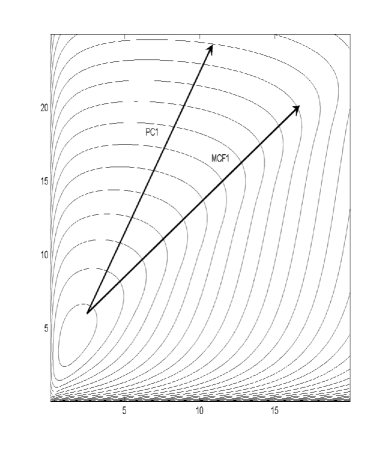
Abbildung 3: Isoprobability contours of the multivariate Gamma distribution, with parameters $\alpha_{0}=2$, $\alpha_{1}=0.5$, $\alpha_{2}=4$. The first principal component is shown (PC1), together with the maximum of the cumulant function (MCF1). All vectors are in arbitrary scale. Again, the maximum of the cumulant function is different from the first principal component, and points towards the large anomalies, in terms of high probability (at fixed, and large, vector norm). Probability contours are $10^{-1/2}$,$10^{-1}$,$10^{-3/2}\ldots$

The cumulant function for this multivariate Gamma distribution can be written (Kotz et al.,, 1998) as

$$\log\Big{\{}\mathbb{E}\big{[}\exp({\bf s}^{t}{\bf X})\big{]}\Big{\}}=-\alpha_{0}\mbox{log}\Big{(}1-\sum_{i=1}^{n}s_{i}\Big{)}-\sum_{i=1}^{n}\alpha_{i}\mbox{log}(1-s_{i})$$

and the mean of the $i^{th}$ component is $\mu_{i}=\alpha_{0}+\alpha_{i}$. By replacing ${\mathbf{s}}$ by $|{\mathbf{s}}|\times\mbox{\boldmath$\theta$}$, the cumulant function of the centered vector $\mbox{\boldmath$\theta$}^{t}({\bf X}-\mbox{\boldmath$\mu$})$ can be written as

$$G_{|{\mathbf{s}}|}(\mbox{\boldmath$\theta$}) = -\alpha_{0}\mbox{log}\Big{(}1-|{\mathbf{s}}|\sum_{i=1}^{n}\theta_{i}\Big{)}$$ (11)

$$- \sum_{i=1}^{n}\alpha_{i}\mbox{log}(1-|{\mathbf{s}}|\theta_{i})-|{\mathbf{s}}|\sum_{i=1}^{n}(\alpha_{0}+\alpha_{i})\theta_{i}.$$

For small $|{\mathbf{s}}|$, the logarithms are approximated by the truncated Taylor expansions, i.e.

$$\sum_{i=1}^{n}\alpha_{i}\mbox{log}\big{(}1-|{\mathbf{s}}|\theta_{i}\big{)}\simeq-|{\mathbf{s}}|\sum_{i=1}^{n}\alpha_{i}\theta_{i}+\frac{|{\mathbf{s}}|^{2}}{2}\sum_{i=1}^{n}\alpha_{i}\theta_{i}^{2}$$

and

$$\alpha_{0}\mbox{log}\big{(}1-|{\mathbf{s}}|\sum_{i=1}^{n}\theta_{i}\big{)}\simeq-|{\mathbf{s}}|\sum_{i=1}^{n}\alpha_{0}\theta_{i}+\frac{|{\mathbf{s}}|^{2}}{2}\alpha_{0}\Big{(}\sum_{i=1}^{n}\theta_{i}\Big{)}^{2}.$$

It follows that the cumulant function can be approximated by

$$G_{|{\mathbf{s}}|}(\mbox{\boldmath$\theta$})\simeq{|{\mathbf{s}}|^{2}\over 2}\mbox{\boldmath$\theta$}^{t}C\mbox{\boldmath$\theta$},$$ (12)

where the covariance matrix $C$ is defined by Kotz et al., (1998)

$$C=\left(\begin{array}[]{lll}\alpha_{0}+\alpha_{1}&&\alpha_{0}\\ &\ddots&\\ \alpha_{0}&&\alpha_{0}+\alpha_{n}\end{array}\right).$$

Hence, for small $|{\mathbf{s}}|$, the solution of (3) is the classical PC1 eigenvector of the covariance matrix $C$ associated with the largest eigenvalue. It is plotted in Figure 3 for the bivariate example. The negative part of PC1 is not displayed, as well as the second principal component which is just orthogonal to the first.

For large $|{\mathbf{s}}|$, the cumulant function is not defined, since the logarithms in Equation (11) must have positive arguments, for all unit vectors $\theta$. In particular, the following two inequalities have to be satisfied

$$|{\mathbf{s}}|\theta_{i}<1\mbox{ and }|{\mathbf{s}}|\sum_{i=1}^{n}\theta_{i}<1.$$

In other words,

$$|{\mathbf{s}}|<\min\left(\min\left({1\over\theta_{i}}\right),{1\over\sum\theta_{i}}\right).$$

However, we take the largest allowed value of $|{\mathbf{s}}|$, which is considered as a valid limit. Since $\theta$ is a unit vector, the maximum of each component $\theta_{i}$ is $1$, which holds when all the other components are zero, while the maximum for the sum $\sum\theta_{i}$ is $\sqrt{n}$, which holds when $\theta_{1}=\theta_{2}=\ldots=\theta_{n}=1/\sqrt{n}$. The largest allowed value of $|{\mathbf{s}}|$ is then $1/\sqrt{n}$: in that case $G$ remains finite for all $\theta$’s, except for $\theta_{1}=\theta_{2}=\ldots=\theta_{n}=1/\sqrt{n}$, where it diverges due to the first logarithm of Equation (11) (all the others remain finite). For larger values of $|{\mathbf{s}}|$, $G$ diverges over subspaces larger than a single point. Hence the boundary case $|{\mathbf{s}}|=1/\sqrt{n}$ is taken as representative for a “large” $|{\mathbf{s}}|$ limit, and the point $\theta_{1}=\theta_{2}=\ldots=\theta_{n}=1/\sqrt{n}$ is taken as the maximum of the cumulant function.

For the bivariate example, the maximum is plotted in Figure 3, denoted as MCF1, and scaled to PC1. Note that for high values of the probability distribution (e.g. the smallest contour), PC1 seems a representative direction of the egg-like shape of the distribution, but for low probabilities it becomes clear that the line $\theta_{1}=\theta_{2}$ is responsible for the large deviations. A point at the end of PC1 is indeed less probable than a point at the end of MCF1.

This result is understood by noting that the joint density (10) is the probability distribution of variables $x_{i}$ defined as $x_{i}=z_{0}+z_{i}$, where the variables $z_{0},z_{1},\ldots,z_{n}$ are independent and Gamma distributed with parameters $\alpha_{0},\alpha_{1},\ldots,\alpha_{n}$. Hence, a large deviation of $z_{0}$, which occurs independently on others $z$’s, corresponds to a large deviation of $\mathbf{x}$ which is placed on average along the line $x_{1}=x_{2}=\ldots=x_{n}$ (that corresponds to $\theta_{1}=\theta_{2}=\ldots=\theta_{n}$ for the cumulant function).

4 Maximizing the marginal density tail

We have seen that the multivariate cumulant function reduces to the variance if the radius $|{\mathbf{s}}|$ tends to zero. In that case, its maxima corresponds to the first principal component of data set. If $|{\mathbf{s}}|$ grows, higher order cumulants come into play, but is not clear what the corresponding maxima represent. In order to clarify this point, we rewrite the cumulant function defined by (2) in terms of the explicit integral over the probability density

$$G_{|{\mathbf{s}}|}(\mbox{\boldmath$\theta$})=\log\int_{\mathbb{R}^{n}}f({\mathbf{x}})\exp(|{\mathbf{s}}|\;\mbox{\boldmath$\theta$}^{t}{\mathbf{x}})d{\mathbf{x}}$$

This expression can be reduced to an unidimensional integral, by defining the projected data as $Z=\mbox{\boldmath$\theta$}^{t}{\mathbf{X}}$, and the marginal probability density of the projected data, $f_{\mbox{\boldmath$\theta$}}(z)$. The cumulant function is then

$$G_{|{\mathbf{s}}|}(\mbox{\boldmath$\theta$})=\log\int_{-\infty}^{+\infty}f_{\mbox{\boldmath$\theta$}}(z)\exp(|{\mathbf{s}}|z)dz,$$ (13)

which corresponds to the cumulant function of the univariate vector $Z=\mbox{\boldmath$\theta$}^{t}{\mathbf{X}}$ with distribution density $f_{\mbox{\boldmath$\theta$}}(z)$. In the light of this representation, our maximization procedure is better understood: we are looking for directions $\theta$ that correspond to a marginal probability density $f_{\mbox{\boldmath$\theta$}}(z)$ displaying maximal cumulant function, at fixed $|{\mathbf{s}}|$. We want to demonstrate that if $|{\mathbf{s}}|$ grows, a larger cumulant function corresponds to a marginal density with a fatter tail. Hence our procedure selects the directions corresponding to the marginal densities with fatter tails, where the anomalous behaviour is expected.

Specifically, consider two different directions $\theta$ and $\theta$^′: we want to demonstrate that if the marginal distribution along $\theta$ has a fatter tail than the distribution along $\theta$^′, then the cumulant function has also a fatter tail along $\theta$ respect to $\theta$^′. More formally, we have the following theorem.

Theorem 1.

Let $\theta$ and ${\mbox{\boldmath$\theta$}^{\prime}}$ be two directions. If there exists a real $z^{*}$ such that the density distribution $f_{\mbox{\boldmath$\theta$}}(z)$ of the random variable $\mbox{\boldmath$\theta$}^{t}{\mathbf{X}}$ is strictly larger than the density $f_{\mbox{\boldmath$\theta$}^{\prime}}(z)$ for all $z>z^{*}$, i.e.

$$f_{\mbox{\boldmath$\theta$}}(z)>f_{\mbox{\boldmath$\theta$}^{\prime}}(z),\;\;\mbox{ for all $z>z^{*}$},$$

then there exists a radius $|{\mathbf{s}}|^{*}$ such the cumulant function of $\mbox{\boldmath$\theta$}^{t}{\mathbf{X}}$ and $\mbox{\boldmath$\theta$}^{\prime t}{\mathbf{X}}$ satisfies

$$G_{|{\mathbf{s}}|}(\mbox{\boldmath$\theta$})>G_{|{\mathbf{s}}|}(\mbox{\boldmath$\theta$}^{\prime}),\;\;\mbox{ for all $|{\mathbf{s}}|>|{\mathbf{s}}|^{*}$.}$$

Beweis.

In order to prove the result, we start by noting that the following inequality holds

$$\exp(|{\mathbf{s}}|z)\big{[}f_{\mbox{\boldmath$\theta$}}(z)-f_{\mbox{\boldmath$\theta$}^{\prime}}(z)\big{]}>\exp(|{\mathbf{s}}|z^{*})\big{[}f_{\mbox{\boldmath$\theta$}}(z)-f_{\mbox{\boldmath$\theta$}^{\prime}}(z)\big{]}$$

for all $z>z^{*}$, where we have replaced the exponential function with its minimum value in the interval $z\in(z^{*},+\infty)$. The inequality holds because the density difference $f_{\mbox{\boldmath$\theta$}}(z)-f_{\mbox{\boldmath$\theta$}^{\prime}}(z)$ is positive in this interval, by assumption. Since the above inequality holds in the whole interval $z\in(z^{*},+\infty)$, it can be integrated over, i.e.

$$\int_{z^{*}}^{+\infty}\exp(|{\mathbf{s}}|z)\big{[}f_{\mbox{\boldmath$\theta$}}(z)-f_{\mbox{\boldmath$\theta$}^{\prime}}(z)\big{]}dz>$$

$$\;\;\;\;\;\;\exp(|{\mathbf{s}}|z^{*})\int_{z^{*}}^{+\infty}\big{[}f_{\mbox{\boldmath$\theta$}}(z)-f_{\mbox{\boldmath$\theta$}^{\prime}}(z)\big{]}dz.$$

Given that the two densities are normalized, i.e.

$$\int_{-\infty}^{+\infty}f_{\mbox{\boldmath$\theta$}}(z)dz=\int_{-\infty}^{+\infty}f_{\mbox{\boldmath$\theta$}^{\prime}}(z)dz=1$$

we can rewrite the right hand side (r.h.s.) of the last inequality by inverting the integration order and the marginal densities as

$$\exp(|{\mathbf{s}}|z^{*})\int_{z^{*}}^{+\infty}\big{[}f_{\mbox{\boldmath$\theta$}}(z)-f_{\mbox{\boldmath$\theta$}^{\prime}}(z)\big{]}dz=$$

$$\exp(|{\mathbf{s}}|z^{*})\int_{-\infty}^{z^{*}}\big{[}f_{\mbox{\boldmath$\theta$}^{\prime}}(z)-f_{\mbox{\boldmath$\theta$}}(z)\big{]}dz$$

Rearranging the four terms gives indeed the normalization condition times the exponential. Note that since the integral in the left hand side (l.h.s.) is, by assumption, positive, the integral in the r.h.s. must be positive as well, because they are multiplied by the same positive constant $\exp(|{\mathbf{s}}|z^{*})$.

Given the above inequalities, we only need to demonstrate that it exists an $|{\mathbf{s}}|^{*}$ such that, for all $|{\mathbf{s}}|>|{\mathbf{s}}|^{*}$,

$$\exp(|{\mathbf{s}}|z^{*})\int_{-\infty}^{z^{*}}\big{[}f_{\mbox{\boldmath$\theta$}^{\prime}}(z)-f_{\mbox{\boldmath$\theta$}}(z)\big{]}dz>$$ (14)

$$\int_{-\infty}^{z^{*}}\exp(|{\mathbf{s}}|z)\big{[}f_{\mbox{\boldmath$\theta$}^{\prime}}(z)-f_{\mbox{\boldmath$\theta$}}(z)\big{]}dz$$

where the value of $|{\mathbf{s}}|^{*}$ must be determined. Note that even if the integral in the l.h.s. is positive, the density difference $f_{\mbox{\boldmath$\theta$}^{\prime}}(z)-f_{\mbox{\boldmath$\theta$}}(z)$ is not guaranteed to be positive for all $z\in(-\infty,z^{*})$. If the integrand was positive as well, Equation (14) would hold trivially for all values of $|{\mathbf{s}}|$, because the exponential in the l.h.s. is always larger than that of r.h.s. This corresponds to the case in which, beside $f_{\mbox{\boldmath$\theta$}}(z)>f_{\mbox{\boldmath$\theta$}^{\prime}}(z)\;\;\;\forall z>z^{*}$, we assume also $f_{\mbox{\boldmath$\theta$}}(z)<f_{\mbox{\boldmath$\theta$}^{\prime}}(z)\;\;\;\forall z<z^{*}$. However, we do not need this additional request, and we just note that it would help our procedure by leaving the problem of using a large $|{\mathbf{s}}|$.

Since the exponential is positive, we can rewrite Equation (14) as

$$\int_{-\infty}^{z^{*}}\big{[}f_{\mbox{\boldmath$\theta$}^{\prime}}(z)-f_{\mbox{\boldmath$\theta$}}(z)\big{]}dz>$$

$$\int_{-\infty}^{z^{*}}\exp\big{(}|{\mathbf{s}}|(z-z^{*})\big{)}\big{[}f_{\mbox{\boldmath$\theta$}^{\prime}}(z)-f_{\mbox{\boldmath$\theta$}}(z)\big{]}dz$$

for all $|{\mathbf{s}}|>|{\mathbf{s}}|^{*}$. The integral in the l.h.s. is positive, as stated above, and is independent on $|{\mathbf{s}}|$, while the integral in the r.h.s. converges to zero for $|{\mathbf{s}}|\longrightarrow+\infty$, as long as the density difference remains finite, because the exponential tends to zero in the whole interval $z\in(-\infty,z^{*})$. If we define $|{\mathbf{s}}|^{*}$ as the largest possible value of $|{\mathbf{s}}|$ for which the two integrals are equal, then for all $|{\mathbf{s}}|>|{\mathbf{s}}|^{*}$ the integral in the l.h.s. is larger than that of r.h.s.

Finally, we have for all $|{\mathbf{s}}|>|{\mathbf{s}}|^{*}$

$$\int_{z^{*}}^{+\infty}dz\;\exp(|{\mathbf{s}}|z)\big{[}f_{\mbox{\boldmath$\theta$}}(z)-f_{\mbox{\boldmath$\theta$}^{\prime}}(z)\big{]}>$$

$$\int_{-\infty}^{z^{*}}dz\;\exp(|{\mathbf{s}}|z)\big{[}f_{\mbox{\boldmath$\theta$}^{\prime}}(z)-f_{\mbox{\boldmath$\theta$}}(z)\big{]}.$$

By rearranging terms, this is equivalent to $G_{|{\mathbf{s}}|}(\mbox{\boldmath$\theta$})>G_{|{\mathbf{s}}|}(\mbox{\boldmath$\theta$}^{\prime})$, and the theorem is demonstrated.

∎

Discussion

In this paper, we have introduced a novel method selecting the spatial patterns representative for the large deviations in the dataset. The method consists in finding the vectors in the space of data for which the cumulant function is maximal. As in the case of PCA, the spatial patterns are found as normalized directions in the space of data, and a linear projection can be performed, with an easy geometrical interpretation. If one is interested on the large deviations, the projection allows to safely perform Extreme Value Analysis (Coles, (2001)). In both cases the subspaces are ordered: in PCA the order follows the fraction of variance of each subspace; The maxima of the cumulant function are ordered by the value of $G$. However, while PCA accounts for the mass of the distribution, the cumulant function can cover the full range of the distribution.

Principal components are always symmetric, while large anomalous patterns, if generated by nonlinear processes, are expected to be neither specular nor orthogonal. Accordingly, the maxima of the cumulant function are not necessarily symmetric, since they account for the whole structure of dependencies, and not only covariances. Other nonsymmetric techniques, such as oblique Varimax rotations, generally depend on the frame of reference: vector solutions do not covary with the space of data under orthogonal transformations. Hence, solutions depend not only on the shape of the underlying probability distribution, but also on its orientation: an undesirable property for our purposes. The maxima of the cumulant function, instead, vary with the probability density whose shape is the only feature determining the maxima.

In the case of normally distributed data, the maximization of cumulant function yields the first principal component for all values of $|s|$: the elliptically symmetric distribution is characterized by the two tails along the major axis of the ellipse, i.e. the first principal component. When the method is applied to Skew-Normal and Gamma distributions, for non-small $|s|$, the maxima of the cumulant function determine large anomalies: high probability directions far from the center of mass. Note that the limit radius $|s|\rightarrow\infty$ is the innovative key from a technical point of view, allowing for analytical solutions. Using the limit, we were also able to demonstrate that the solutions of our algorithm correspond, in general, to the directions along which the marginal probability density display the fattest tails.

Using the cumulant function is computationally cheap, there is no free parameter, and has the advantage of searching for local solutions, all of which are of interest. When a solution is found, is always a good solution, in contrast with neural networks applications, for which it must be questioned if it is the global or just a local solution. In real applications (see Bernacchia et al.,, 2007), the radius $|s|$ must be taken as large as possible, until the expected error in the estimate of the cumulant function, due to the finite sample, reach a tolerance value (see Bernacchia et al.,, 2007). This corresponds to maximize a combination of cumulants which is of the highest reliable order with the given amount of data, accounting for the available set of anomalies.

The solutions of our algorithm are expected to transform continuously as the radius $|s|$ varies. Hence, even if the limit $|s|\rightarrow\infty$ cannot be taken in practice, the solutions for a finite value of $|s|$ are expected to represent a substantial departure from the PCA solution, towards the formal solution at $|s|\rightarrow\infty$. From the theoretical point of view, future work could be devoted to studying more in detail the nature of solutions at varying $|s|$. For instance, one could attempt to find under which conditions and to what extent the solutions are in between the PCA solution and the formal solution at infinite $|s|$. From the applicative point of view, we expect several datasets (e.g. Bernacchia et al.,, 2007) to be fruitfully analyzed with our new method.

Note that the logarithm is taken for illustrative purposes: the moment generating function could be used instead of the cumulant function, since the maximization is invariant under application of a monotonous function. The present definition is however confortable in avoiding extremely large numbers. Centering of data about the mean is also a practical step, related with the constraint of dealing with finite samples: if the limit $|s|\rightarrow\infty$ could be really taken, the mean would be irrelevant.

Results of our procedure are corrupted if variables are standardized by a rescaling, since the relative scale of different directions is the key in detecting anomalies and comparing the size of tails. If variables are standardized, our procedure reduce to a special case of Independent Component Analyisis (ICA, see Hyvarinen and Oja, (2007)), detecting independent components rather than large anomalies. Results are also corrupted if we try to get an empirical estimate of the cumulant function when the underlying probability density decays less than exponentially fast. In that case, the cumulant function diverge, and the variance of the empirical estimate increases with the size of the sample (Sornette, (2000)), implying that the estimate is always unreliable.