Selection of dominant multi-exciton transitions in disordered linear J-aggregates

Abstract

We show that the third-order optical response of disordered linear J-aggregates can be calculated by considering only a limited number of transitions between (multi-) exciton states. We calculate the pump-probe absorption spectrum resulting from the truncated set of transitions and show that, apart from the blue wing of the induced absorption peak, it agrees well with the exact spectrum.

1 Introduction

Since the discovery of the J-band of pseudoisocyanine (PIC) [1, 2], the study of the collective optical properties of molecular aggregates has received much attention. The collective nature of the excitations gives rise to narrow absorption lines (exchange narrowing) and ultra-fast spontaneous emission. The development of novel optical techniques, a continuously increasing theoretical understanding of the optical response of these systems, and the realization that this type of excitations play an important role in natural light harvesting systems have kept these materials in the spotlight.

During the past 15 years a topic of particular interest has been the effect of multi-exciton states on nonlinear optical spectroscopies. Amongst the latter are the nonlinear absorption spectrum [3, 4], photon echoes [5, 6], pump-probe spectroscopy [6, 7, 8], and two-dimensional spectroscopy [9, 10]. From a theoretical point of view, accounting for multi-exciton states requires the handling of large matrices, due to the extent of the associated Hilbert space. It is well-known, however, that for homogeneous linear aggregates, three states dominate the third-order response, namely the ground state, the lowest one-exciton state and the lowest two-exciton state. In practice, J-aggregates suffer from appreciable disorder, which leads to localization of the exciton states. It was shown in Ref. [7] that the three-state picture still holds to a good approximation, provided that one replaces the chain length by the typical exciton localization length. The existence of the so-called hidden structure of the Lifshits tail of the density of states (DOS) justifies this approach [11, 12].

In this paper, we put a firmer basis under the above idea, by systematically analyzing the dominant ground-state to one-exciton transitions and one- to two-exciton transitions in disordered linear aggregates. By comparison to exact spectra, we show that, indeed, the picture of three dominant states per localization segment holds.

2 Model

We model a single aggregate as a linear chain of $N$ coupled two-level monomers with parallel transition dipoles. We assume that the aggregate interacts with a disordered environment, resulting in random fluctuations in the molecular transition energies $\varepsilon_{n}$ (diagonal disorder), and restrict ourselves to nearest neighbor excitation transfer interactions $-J$. The optical excitations are described by the Frenkel exciton Hamiltonian,

$$H=\sum_{n=1}^{N}\varepsilon_{n}|n\rangle\langle n|-J\sum_{n=1}^{N-1}\left(|n\rangle\langle n+1|+h.c.\right).$$ (1)

Here, $|n\rangle$ denotes the state with the $n$th site excited and all other sites in the ground state. The monomer excitation energies $\varepsilon_{n}$ are modeled as uncorrelated Gaussian variables with zero mean and standard deviation $\sigma$. For J-aggregates $J>0$. Numerical diagonalization of the Hamilton yields the exciton energies $\varepsilon_{\nu}$ ($\nu=1,\ldots,N$) and exciton wavefunctions $|\nu\rangle=\sum_{n=1}^{N}\varphi_{\nu n}|n\rangle$ of the one-exciton states, where $\varphi_{\nu n}$ is the $n$th component of the wavefunction $|\nu\rangle$. The two exciton states are given by the Slater determinant of two different one-exciton states $|\nu_{1}\rangle$ and $|\nu_{2}\rangle$ [4]: $|\nu_{1},\nu_{2}\rangle=\sum_{n\leq m}^{N}(\phi_{\nu_{1}n}\phi_{\nu_{2}m}-\phi_{\nu_{1}m}\phi_{\nu_{2}n})|n,m\rangle$ with $|n,m\rangle$ the state in which the sites $n$ and $m$ are excited and all other sites are in the ground state. The corresponding two-exciton energy is given by $E_{\nu_{1}\nu_{2}}=E_{\nu_{1}}+E_{\nu_{2}}$.

3 Selecting dominant transitions

The physical size of a molecular aggregate can amount to thousands of monomers, but the disorder localizes the exciton states [13]. For J-aggregates a small number of states at the bottom of the one-exciton band contain almost all the oscillator strength. The states are localized on segments with a typical extension $N^{*}$, called the localization length, which depends on the magnitude of the disorder [14]. The wavefunctions of these states overlap weakly and consist of (mainly) a single peak (they have no node within the localization segment), see Fig. 2. For the remainder of this paper we will refer to these states as $s$ states, and $\mathcal{S}$ will denote the set of $s$ states.

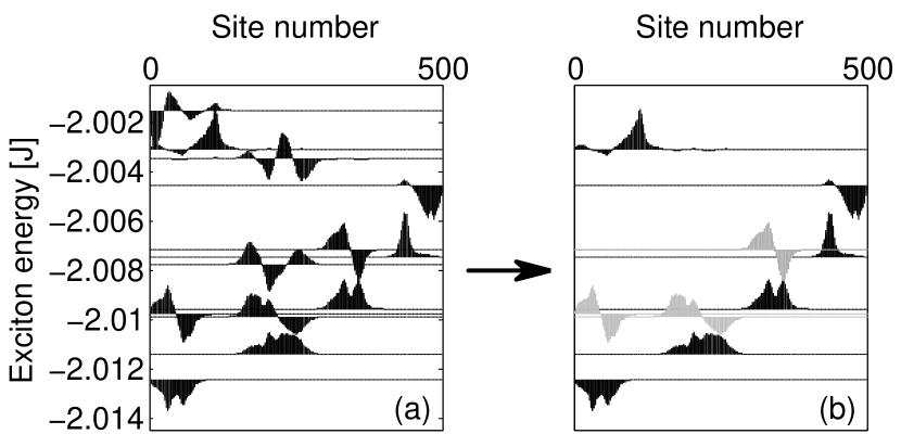
Figure 1:

Figure 2: (a) The lowest 12 one-exciton states of a chain of length $N=500$ for a particular disorder realization. (b) A subset of $s$ states (black) and $p$ states (gray) that mostly contribute to the one-to-two exciton transitions.

From the complete set of wavefunctions we select the $s$ states using the selection rule proposed in Ref. [12], $\big{|}\sum_{n}\varphi_{\nu n}|\varphi_{\nu n}|\big{|}\geq C_{0}$. For a disorder-free the lowest state contains 81% of the total oscillator strength between the ground state and the one-exciton band [14]. Numerically we found that the $s$ states selected by taking $C_{0}=0.75$ (for $0.05J<\sigma<0.3J$) together contain 76% of the total oscillator strength: ${\langle\sum_{s\in\mathcal{S}}\mu_{s}^{2}\rangle}/{N}\approx 0.76$. Here $\mu_{s}$ is the transition dipole moment from the ground state to the state $|s\rangle$. In Fig. 4(a) we show the absorption spectrum calculated only with the $s$ states and compare it to the exact spectrum.

We observe that the $s$ states give a good representation of this spectrum, except for its blue wing, where higher-energy exciton states, which contain one node within the localization segment, contribute as well [15, 16]. These so-called $p$ states may be identified as the second one-exciton state on a localization segment [11, 12].

The $p$ states play a crucial role in the third-order response. In order to analyze this, we have considered two-exciton states $|s,p\rangle$ given by the Slater determinant of a given $s$ state (selected as described above) with all other one-exciton states $\nu\notin\mathcal{S}$ (the two-exciton state consisting of two $s$ type states localized on different segments do not contribute to the nonlinear response), and calculate the corresponding transition dipole moments $\mu_{s\nu,s}$. From the whole set of $\mu_{s\nu,s}$, we select the largest one, denoted by $\mu_{sp_{s},s}$, were the substrict $s$ in $p_{s}$ indicates its relation with the state $|s\rangle$. It turns out that the one-exciton state $|p_{s}\rangle$ selected in this way is localized on the same segment as the state $|s\rangle$. Several of these doublets of $s$ and $p$ states are shown in Fig. 2(b). The partners of the lowest $s$ states indeed look like $p$ states, having a well-defined node within the localization segment. They form the hidden structure of the Lifshits tail of the DOS [11] we mentioned above. For higher lying $s$ states, these partners (not shown) are more delocalized and often do not have a $p$-like shape.

The average ratio of the oscillator strength of the transitions $|0\rangle\to|s\rangle$ and $|s\rangle\to|p_{s}\rangle$ turned out to be $\left\langle{\mu_{sp_{s},s}^{2}}/{\mu_{s}^{2}}\right\rangle\approx 1.4$. For the dominant ground-to-one and one-to-two exciton transition in a homogeneous chain, this ratio reads ${\mu_{12,1}^{2}}/{\mu_{1}^{2}}\approx 1.57$. This comparison suggests that our selection of two-exciton states well captures the dominant one-to-two exciton transitions in disordered chains. We have also found that the energy separation between the states $|s\rangle$ and $|p_{s}\rangle$ obeys $\left\langle E_{s}-{E_{p_{s}}}\right\rangle\approx 1.35\times{3\pi^{2}J}/{N^{*2}}$, with $N^{*}=\left\langle{\mu_{s}^{2}}/{0.81}\right\rangle$. This resembles the level spacing of a homogeneous chain: $E_{2}-{E_{1}}\approx{3\pi^{2}J}/{N^{2}}$, confirming that the separation between the one-exciton bleaching peak and the one-to-two-exciton induced absorption peak may be used to extract the typical localization size from experiment [8].

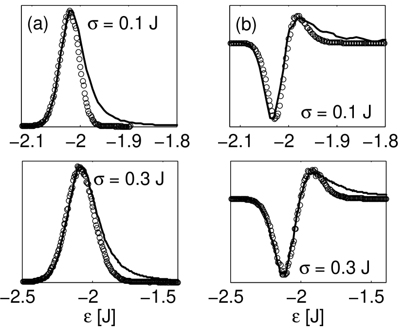
Figure 3:

Figure 4: (a) Absorption spectrum due to $s$ states (circles) compared to the exact one (solid line). (b) Pump-probe spectrum due to the selected $s$ and $p$ type states (circles) compared to the exact one (solid line). The spectra were calculated for $\sigma=0.1J$ (top) and $\sigma=0.3J$ (bottom).

To illustrate how the selected transitions, involving the ($s$,$p$) doublets, reproduce the optical response of the aggregate, we have calculated the pump-probe spectrum at zero temperature using only these transitions [10],

$$P(\omega)=\bigg{\langle}-2\mu_{s}^{4}\delta(\omega_{s}-\omega)+\mu_{s}^{2}\mu_{p_{s}}^{2}\delta(\omega_{p_{s}}-\omega)\bigg{\rangle},$$ (2)

and compared the result to the exact spectrum, see Fig. 4(b). Apart from a blue wing in the induced absorption part of the spectrum (the positive peak), the selected transitions reproduce the exact pump-probe spectrum very well. In particular the separation between the bleaching and induced absorption peaks is practically identical to the exact one.

4 Conclusion

We have shown that the third-order optical response of disordered linear J-aggregates is dominated by a very limited number of transitions. Considering only these transitions enormously reduces the computational effort necessary to simulate nonlinear experiments. We have used the procedure outlined above to calculate the optical bistable response of a thin film of J-aggregates, taking into account the one-to-two exciton transitions [16].

References

- [1] E. E. Jelley, Nature 139, 631 (1937).
- [2] G. Scheibe, Angew. Chem. 50, 212 (1937).
- [3] F. C. Spano , and S. Mukamel, Phys. Rev. A 40, 5783 (1989).
- [4] F. C. Spano, Phys. Rev. Lett. 67, 3424 (1991).
- [5] F. C. Spano, J. Chem. Phys. 96, 2845 (1992).
- [6] M. van Burgel, D. A. Wiersma, and K. Duppen, J. Chem. Phys.102, 20 (1995).
- [7] H. Fidder, J. Knoester, and D. A. Wiersma, J. Chem. Phys. 98, 6564 (1993).
- [8] L. Bakalis, and J. Knoester J. Phys. Chem. B 103, 6620 (1999).
- [9] T. Brixner et al, J. Phys. Chem. B 110, 20032 (2006).
- [10] D. J. Heijs, A. G. Dijkstra, and J. Knoester, accepted by Chem. Phys.
- [11] V. Malyshev and P. Moreno, Phys. Rev. B 51 14587 (1995).
- [12] A. V. Malyshev and V. A. Malyshev, Phys. Rev. B 63 195111 (2001).
- [13] E. Abrahams et. al., Phys. Rev. Lett. 42, 679 (1979).
- [14] H. Fidder, J. Knoester, and D. A. Wiersma, J. Chem. Phys. 95, 7880 (1991).
- [15] A. V. Malyshev, V. A. Malyshev and J. Knoester, Phys. Rev. Lett. 98, 087401 (2007).
- [16] J. A. Klugkist, V. A. Malyshev, and J. Knoester, in preparation.