Probabilistic Robustness Analysis — Risks, Complexity and Algorithms

Abstract.

It is becoming increasingly apparent that probabilistic approaches can overcome conservatism and computational complexity of the classical worst-case deterministic framework and may lead to designs that are actually safer. In this paper we argue that a comprehensive probabilistic robustness analysis requires a detailed evaluation of the robustness function and we show that such evaluation can be performed with essentially any desired accuracy and confidence using algorithms with complexity linear in the dimension of the uncertainty space. Moreover, we show that the average memory requirements of such algorithms are absolutely bounded and well within the capabilities of today’s computers.

In addition to efficiency, our approach permits control over statistical sampling error and the error due to discretization of the uncertainty radius. For a specific level of tolerance of the discretization error, our techniques provide an efficiency improvement upon conventional methods which is inversely proportional to the accuracy level; i.e., our algorithms get better as the demands for accuracy increase.

1. Introduction

In recent years, a number of researchers have proposed probabilistic control methods for overcoming the computational complexity and conservatism of the deterministic worst-case robust control framework (e.g., [1]–[7], [11]–[20] and the references therein).

The philosophy of probabilistic control theory is to sacrifice cases of extreme uncertainty. Such paradigm has lead to the concept of confidence degradation function (originated by Barmish, Lagoa and Tempo [2]), which has demonstrated to be extremely powerful for the robustness analysis of uncertain systems. Such function, $\mathscr{P}(.)$, is defined as $\mathscr{P}(r)=\inf_{0<\rho\leq r}\mathbb{P}(\rho)$ with

$$\mathbb{P}(\rho)=\mathrm{vol}\{\text{$X\in\mathcal{B}_{\rho}\mid$ The robustness requirement is guaranteed for $X$}\}/\mathrm{vol}\{\mathcal{B}_{\rho}\}$$

where the volume function $\mathrm{vol}\{.\}$ is the Lebesgue measure, and $\mathcal{B}_{\rho}$ denotes the uncertainty bounding set with radius $\rho$. Interestingly, it was discovered in [2] that such function is not necessarily monotone decreasing in the uncertainty radius. In view of this fact and for the purpose of avoiding the confusion with the concept of confidence band, used in the evaluation of the accuracy of the estimate of $\mathbb{P}(r)$, the confidence degradation function is referred to as the robustness function in this paper. Accordingly, a graph representation of the robustness function is called the robustness curve. It can be seen that the robustness function is a natural extension of the concept of robustness margin. From the robustness curve, one can determine the probabilistic robustness margin [2] and estimate the deterministic robustness margin.

In addition to overcoming the NP hard complexity and conservatism of deterministic robustness analysis methods, the robustness function can address very complex problems which are intractable by deterministic worst-case methods. Moreover, the probability that the robustness requirement is guaranteed can be inferred from the robustness function, while the deterministic margin losses the connection with such probability. Based on the assumption that the density function of uncertainty is radially symmetric and non-increasing with respect to the norm of uncertainty, it has been shown in [2] that the probability that the robustness requirement is guaranteed is no less than $\mathscr{P}(r)=\inf_{\rho\in(0,r]}\mathbb{P}(\rho)$ when the uncertainty is included in a bounding set with radius $r$. The underlying assumption is supported by modeling and manufacturing considerations that the uncertainty is unstructured so that all directions are equally likely and that small perturbations from the nominal model are more likely than large perturbations. Since $\mathbb{P}(.)$ is not monotonically decreasing [2], the lower bound of the probability depends on $\mathbb{P}(\rho)$ for all $\rho\in(0,r]$. It is not clear whether it is feasible to estimate $\mathscr{P}(r)$ since the estimation of $\mathbb{P}(\rho)$ for every $\rho$ relies on intensive Monte Carlo simulation and $\mathbb{P}(\rho)$ needs to be estimated for numerous values of $\rho$. For such probabilistic method to overcome the NP hard of worst-case methods, it is necessary to show that the complexity for estimating $\mathscr{P}(r)$ for a given $r$ is polynomial in terms of computer running time and memory space. In this paper, we demonstrate that the complexity in terms of space and time is surprisingly low and is linear in the uncertainty dimension and the logarithm of the relative width of the range of uncertainty radius.

In the next section we argue that both the deterministic robustness margin and its risk-adjusted version – the probabilistic robustness margin have inherent limitations. We address those limitations through the use of the robustness function that can describe the performance of a system over a wide range of uncertainties. In order to construct the robustness function for wide range of uncertainty radii, the conventional method independently estimate $\mathbb{P}(r_{i})$ for each grid points of uncertainty. If there are $m$ grid points and $N$ is the sample size for each radius, then the total number of simulations is $Nm$. In Section 3, we use the sample reuse principle and demonstrate that the robustness curve for arbitrarily wide range of uncertainty radii can be accurately constructed with surprisingly low complexity. Clearly, the number of grid points, $m$, must tend to infinity as the tolerance tends to zero. However, we show that with our algorithms, the equivalent number of grid points (ENGP), $m_{eq}$, is strictly bounded from above in the sense that in order to guarantee the same level of accuracy for the estimation of the robustness function, the required average computational effort is the same as that of a conventional grid with $m_{eq}$ points. Moreover, we show that the average memory requirement is also absolutely bounded and is well within the reach of modern computers.

The remainder of the paper is organized as follows. Section 2 provides an example illustrating the pitfalls of deterministic robustness margin and the probabilistic robustness margin. Section 4 discusses the control of estimation error of the robustness function and the required complexity. Section 5 investigates the difficulties of the conventional data structure. Section 6 describes our new algorithms, analyzes the complexity of data processing and memory space, and introduces the concept of confidence band. The proofs of all the theorems are included in the Appendices.

2. The Risk of Robustness Margins

In this section we make the case for the need to have a robustness function in order to properly estimate how well a control system tolerates uncertainties. Conventional robust control approaches the issue with a “worst case” philosophy. In this regard, it has been demonstrated (Chen, Aravena and Zhou, [5]) that it is not uncommon for a probabilistic controller to be significantly less risky than a deterministic worst-case control. The reasons are the “uncertainty in modeling uncertainties” and the fact that the worst-case design cannot, in some instances, be “all encompassing.” Therefore, the worst-case approach has an associated risk that usually is overlooked, while the probabilistic approach acknowledges the risk and manages it.

From manufacturing and modeling considerations, it is sensible to assume that the density of the distribution of uncertainty decreases with increasing uncertainty norm. Such assumption leads to the worst-case property of uniform distribution in robustness analysis [2]. However, the decay rate of density is generally unknown to the designer. Therefore, for a given uncertainty radius $r$, one does not have good knowledge about the coverage probability of the uncertainty set $\mathcal{B}_{r}$. It is important to note that the system robustness depends critically on the distribution of uncertainty norm.

Attempts to improve the analysis have led to the definitions of a deterministic robustness margin and a probabilistic robustness margin. Both are numbers that purportedly allow the user to estimate the tolerance to uncertainties. We contend that both can be misleading, and for essentially the same reason. To demonstrate this view point, we consider a feedback system shown in Figure 1.

Figure 1. Standard Feedback Configuration

The transfer function of the plant is $G(s)=\frac{q}{s-p}$ where $p$ and $q$ are uncertain parameters. The uncertainty bounding set with radius $r>0$ is

$$\mathcal{B}_{r}=\{(x,y):\;|x-q_{0}|\leq r,\quad|y-p_{0}|\leq r\},\qquad p_{0}<0,\qquad q_{0}>0.$$

Consider two controllers $C_{A}=\frac{K_{A}}{s+\sigma},\quad\sigma>0$ and $C_{B}=K_{B}$ such that

$$1<K_{B}<\frac{K_{A}}{\sigma},\qquad\frac{K_{A}\;q_{0}-\sigma\;p_{0}}{K_{A}+\sigma}<\sigma-p_{0}.$$

Suppose that the robustness requirement is stability. It can be shown that the robustness function for controller $A$ is

$$\mathscr{P}^{A}(r)=\begin{cases}1&\text{for}\quad 0<r<\rho_{A};\\ \frac{1}{2}-\frac{K_{A}\left(r+\frac{\sigma\;\beta}{K_{A}}-q_{0}\right)^{2}}{8\sigma\;r^{2}}-\frac{p_{0}-\beta}{2r}&\text{for}\quad\rho_{A}\leq r\leq\rho_{A}^{*};\\ \frac{1}{2}-\frac{(r+\beta-p_{0})\left(r+\frac{\sigma(\beta+p_{0}-r)}{2K_{A}}-q_{0}\right)}{4r^{2}}-\frac{(p_{0}-\beta)}{2r}&\text{for}\quad r>\rho_{A}^{*}\end{cases}$$

where

$$\rho_{A}=\frac{K_{A}\;q_{0}-\sigma\;p_{0}}{K_{A}+\sigma}$$

is the deterministic robustness margin, $\beta=\min(\sigma,p_{0}+r)$, and $\rho_{A}^{*}=\frac{K_{A}\;q_{0}-\sigma\;p_{0}}{K_{A}-\sigma}$. It can be shown that the robustness function for controller $B$ is given by

$$\mathscr{P}^{B}(r)=\begin{cases}1&\text{for}\quad 0<r<\rho_{B};\\ 1-\frac{K_{B}\left(r+\frac{p_{0}+r}{K_{B}}-q_{0}\right)^{2}}{8r^{2}}&\text{for}\quad\rho_{B}\leq r\leq\rho_{B}^{*};\\ \frac{1}{2}-\frac{\frac{p_{0}}{K_{B}}-q_{0}}{2r}&\text{for}\quad r>\rho_{B}^{*}\end{cases}$$

where

$$\rho_{B}=\frac{K_{B}\;q_{0}-p_{0}}{K_{B}+1}$$

is the deterministic robustness margin and $\rho_{B}^{*}=\frac{K_{B}\;q_{0}-p_{0}}{K_{B}-1}$.

We consider an example with $p_{0}=-10,\;q_{0}=50,\;\sigma=40,\;K_{A}=100\sigma,\;K_{B}=10$. The corresponding robustness functions are displayed in Figure 2. We obtained deterministic margins $\rho_{A}=49.6040,\;\rho_{B}=46.3636$. Since $\rho_{A}>\rho_{B}$, a comparison based on the deterministic margin simply suggests that controller $A$ is more robust than controller $B$. Quite contrary, a judgement based on the robustness curves indicates that controller $B$ may be more robust. The risk of the probabilistic robustness margin can also be illustrated by this example.

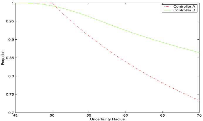
Figure 2. Comparison of Controller Alternatives.

Robust analysis should be able to help a designer to reliably determine which controller design is more robust. However, it appears that the concepts of robustness margin fail to meet such fundamental needs of control engineering. On the other hand, the robustness curve serves the purpose of giving the designer complete information on how well a control system tolerates uncertainties.

From the previous discussion, it can be seen that there are two crucial factors to be considered in order to make a reliable judgment about the system robustness:

(i):

How fast the robustness curve rolls off.

(ii):

The dependency of coverage probability of uncertainty bounding set $\mathcal{B}_{r}$ on the radius $r$.

The second factor can be a difficulty since a designer generally lacks knowledge of the coverage probability corresponding to a bounding set of fixed radius. To overcome such difficulty, the only choice is to construct the robustness curve for a wide range of uncertainty radius. The construction of the robustness curve may be seen as a computationally challenging task since the probability of guaranteeing robustness requirement needs to be estimated for many values of uncertainty radius. However, as we demonstrate in the next section, using the sample reuse principle one can construct the robustness curve for virtually the entire scope of uncertainty range $(0,\infty)$ with absolutely bounded average computational requirements, regardless of the size of the grid. For example, we shall show that for an uncertainty range as large as $(10^{-10},\;10^{10})$, in the average, one needs less than 50 times memory and computational resources than those needed to evaluate the uncertainty range $(1,\;e)$ with the same resolution.

3. Equivalent Number of Grid Points

Throughout this paper, we assume that the uncertainty sets are homogeneous star-shaped (e.g., [2]). That is, the uncertainty bounding set with radius $r$ is $\mathcal{B}_{r}=\{rX\mid X\in\mathcal{B}_{1}\}$ where $\mathcal{B}_{1}$ denotes the uncertainty bounding set such that $cX\in\mathcal{B}_{1}$ for any $X\in\mathcal{B}_{1}$ and any $c\in[0,1]$. Clearly, most of the commonly used uncertainty bounding sets such as the $l_{p}$ balls and spectral norm balls are homogeneous star-shaped.

We shall consider the problem of constructing the robustness curve for arbitrary robustness requirement $\mathbf{P}$ under such assumption of uncertainty sets. Conventionally, the robustness curve for a range of uncertainty radii $\left[\frac{a}{\lambda},\;a\right]$ with $a>0,\;\lambda>1$ is constructed by choosing a set of grid points $\frac{a}{\lambda}=r_{1}<r_{2}<\cdots<r_{m}=a$ and, for every grid point, performing $N$ i.i.d. Monte Carlo simulations. Hence, the total number of simulations is a deterministic constant $mN$. To reduce computational complexity, we shall make use of the following intuitive concept:

Let $X$ be an observation of a random variable with uniform distribution over $\mathcal{B}_{\rho}\supseteq\mathcal{B}_{r}$ such that $X\in\mathcal{B}_{r}$. Then $X$ can also be viewed as an observation of a random variable with uniform distribution over $\mathcal{B}_{r}$.

In order to apply such concept, it is necessary to perform the simulation in a backward direction so that appropriate evaluations of the robust requirement for larger uncertainty sets can be saved for the use of later simulations on smaller uncertainty sets [6]. The sample reuse principle allows a single simulation to be used for multiple radii. Thus, the actual total number of simulations is significantly reduced. In order to quantify this reduction we introduce the equivalent number of grid points (ENGP), $m_{eq}$, defined as

$$m_{eq}=\frac{\mbox{expected total number of simulations}}{N}.$$

In our approach, the number of simulations required at uncertainty radius $r_{i}$, denoted by ${\bf n}_{i}$ for $i=1,\cdots,m$, is a random number. The total number of simulations can be represented by the random variable $\boldsymbol{n}=\sum_{i=1}^{m}{\bf n}_{i}$. The expected value of the total number of simulations is $\mathbb{E}[\boldsymbol{n}]=\sum_{i=1}^{m}\mathbb{E}[{\bf n}_{i}]$ where $\mathbb{E}[X]$ denotes the expectation of random variable $X$. Hence, we can formally define

$$m_{eq}=\frac{\mathbb{E}[\boldsymbol{n}]}{N}.$$

Due to sample reuse, we can achieve a substantial reduction of simulations, i.e., $\mathbb{E}[\boldsymbol{n}]<<mN$. To quantify the reduction of the computational effort, we have introduced the notion of sample reuse factor [6], which is defined as

(3.1) $$\mathcal{F}_{\mathrm{reuse}}\stackrel{{\scriptstyle\mathrm{def}}}{{=}}\frac{mN}{\mathbb{E}[\boldsymbol{n}]}=\frac{m}{m_{eq}}.$$

In our approach, $N$ i.i.d simulation results are collected for each grid point. Hence, the accuracy of estimation is the same as that of the conventional method. However, the average number of simulations in our approach is $\mathbb{E}[\boldsymbol{n}]$, which is equivalent to the complexity of $m_{eq}$ grid points in the conventional scheme. As a direct consequence of Theorem 1 of [6], we have that, for any discretization scheme, $m_{eq}$ is independent of the sample size $N$. Moreover, we have the following general results.

Theorem 1.

Let $d$ be the dimension of uncertainty parameter space. Then, for arbitrary gridding scheme, the equivalent number of grid points based on the principle of sample reuse is strictly bounded from above by $1+d\;\ln\lambda$, i.e.,

$$m_{\mathrm{eq}}<1+d\;\ln\lambda.$$

See Appendix A for a proof. By an “arbitrary” discretization scheme, we mean two things: i) the number of grid points can be arbitrarily large; ii) the grid points can be distributed arbitrarily over the specified range of uncertainty radius.

A fundamental question of robust control is whether randomized algorithms have polynomial complexity. In light of the fact the cost of each simulation depends on problem cases, the computational complexity is usually measured in terms of the number of simulations. This theorem reveals the following important facts:

(a):

The complexity is linear in the dimension of the uncertainty space. Thus our algorithms overcome the curse of dimensionality.

(b):

The complexity depends linearly in the logarithm of the “relative” width, $\lambda$, of the interval of uncertainty radii. This proves that our algorithms are capable of estimating the robustness function for a wide range of uncertainty.

(c):

Our algorithms can arbitrarily reduce the grid error, while keeping the complexity strictly below a constant bound.

In order to illustrate these points, Figure 3 displays the variation of $m_{eq}$ for various dimensions of the uncertainty space and for values of $\lambda$ up to $\lambda=10^{20}$ corresponding to the uncertainty range $(10^{-10},10^{10})$ (which may be deemed a good approximation to $(0,\infty)$). Notice that even for dimensions as high as $d=1024$ the equivalent number of grid points, $m_{eq}$, is very reasonable.

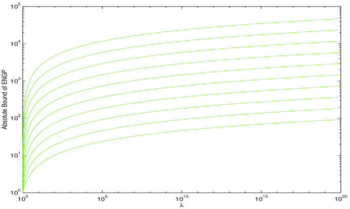
Figure 3. Absolute Bounds for $m_{eq}$ (ENGP) ($d=2^{i},\;i=1,\cdots,10$).

Finally in this section, we consider the case where we need to estimate $\mathbb{P}(r)$ for $r\in[\gamma,U]$ where $\gamma>0$ is a constant, and $U$ is an estimate of the probabilistic robustness margin calculated by randomized algorithms. Clearly, $U$ is a random variable. If $U$ depends on samples which are independent of the samples generated from the uncertainty set with radius $r\in[\gamma,U]$ we have the following result:

For any gridding scheme,

(3.2) $$m_{eq}<1+d\ln\frac{\mathbb{E}[U]}{\gamma}.$$

To prove (3.2), notice that $\mathbb{E}[\mathbb{E}[X\mid Y]]=\mathbb{E}[X]$ for any random variables $X$ and $Y$. Hence, by Theorem 1,

$$m_{\mathrm{eq}} = \mathbb{E}[\mathbb{E}[m_{\mathrm{eq}}\mid U]]<\mathbb{E}\left[1+d\ln\frac{U}{\gamma}\right]=1+d\;\mathbb{E}\left[\ln\frac{U}{\gamma}\right]<1+d\ln\frac{\mathbb{E}[U]}{\gamma}$$

where the last inequality is obtained from applying the Jensen’s inequality to the concave function $\ln(.)$.

4. Error Control

In addition to efficiency, another important issue in any numerical approach is error control. This point has been emphasized in many control engineering problems. For instance, when computing the $H_{\infty}$ norm of a system, a lower bound and an upper bound are obtained and is required that the gap between them be less than a prescribed tolerance. A similar situation arises in the computation of the structured singular value $(\mu)$.

For the specific case of the estimation of the robustness function, there are two sources of error: i) the statistical sampling error due to the finiteness of the sample size, $N$ (sample size error); ii) the discretization error due to the finite number of points in any partition. Control of the sample size error has been well studied and emphasized. Existing techniques include the Chernoff bounds [8], binomial confidence interval [7, 9], etc. However, we claim that control of discretization error is not sufficiently emphasized. In fact, one can argue that controlling the sample size error can be meaningless if the discretization error is not controlled. This will be the case, for example, for those situations where a risk at the level of a small $\varepsilon$ (e.g., $\varepsilon=0.001$) may be significant or unacceptable. How can any estimation be useful if the discretization error is not ensured to be less than the tolerance $\varepsilon$ ?

In this section, we first introduce an interpolation result necessary to analyze error control methods. Afterward, we discuss two different schemes which insure a discretization error less than a given $\epsilon\in(0,1)$. The first is a uniform partition whereby the uncertainty radius interval $[\frac{a}{\lambda},a]$ is partitioned by $m$ points

(4.1) $$r_{i}=a-\frac{(m-i)(\lambda-1)}{(m-1)\lambda}a,\qquad i=1,\cdots,m.$$

In the second scheme we consider a geometric type partition of the form

(4.2) $$r_{i}=a\left(\frac{1}{\lambda}\right)^{\frac{m-i}{m-1}},\qquad i=1,\cdots,m.$$

For any partition of the uncertainty radius interval, we have the following linear interpolation results.

Theorem 2.

Given an arbitrary partition of the uncertainty radius interval $\left[\frac{a}{\lambda},\;a\right]$ with $\frac{a}{\lambda}=r_{1}<r_{2}<\cdots<r_{m}=a$, define

$$\mathbb{P}^{*}(r)=\frac{(r-r_{i})\;\mathbb{P}(r_{i+1})+(r_{i+1}-r)\;\mathbb{P}(r_{i})}{r_{i+1}-r_{i}},$$

$$g(r)=(r_{i+1}-r)\left(\frac{r}{r_{i}}\right)^{-d}+(r-r_{i})\left(\frac{r_{i+1}}{r}\right)^{-d}.$$

Then, for all $r\in[r_{i},r_{i+1}]$,

$$|\mathbb{P}(r)-\mathbb{P}^{*}(r)|\leq 1-\frac{g(r_{\star})}{r_{i+1}-r_{i}}\leq\frac{d}{2r_{i}}(r_{i+1}-r_{i})$$

where $r_{\star}\in(r_{i},r_{i+1})$ is the unique solution of equation

$$\left(\frac{r_{i+1}}{r}\right)^{-d}\left[1+\left(1-\frac{r_{i}}{r}\right)d\right]-\left(\frac{r}{r_{i}}\right)^{-d}\left[1+\left(\frac{r_{i+1}}{r}-1\right)d\right]=0$$

with respect to $r$, which can be solved by a bisection search.

See Appendix B for a proof. As mentioned before, these interpolation results will be used in the construction of a tight confidence band for the robustness function.

Remark 1.

To guarantee a prescribed tolerance $\epsilon\in(0,1)$, the number of grid points must be larger than a certain number. It has been shown by Barmish, Lagoa and Tempo [2] that if

(4.3) $$m\geq 1+\frac{2(\lambda-1)d}{\epsilon}$$

then $|\mathbb{P}(r)-\mathbb{P}(r_{i})|<\epsilon\quad\forall r\in[r_{i},r_{i+1}]$ for $i=1,\cdots,m-1$. This bound shows that, for fixed error $\epsilon$, the complexity is polynomial. From another perspective, it also shows that the number of grid points and computational complexity tend to infinity as the tolerance tends to zero. For example, the robustness analysis problem for complex uncertainty of size $30\times 30$ over an interval of uncertainty with $\lambda=10$, requires $m\geq 3,240,000,001$ in order to guarantee $\epsilon\leq 10^{-5}$. The bound, however, does not account for the sample reuse principle. Using our approach the equivalent number of grid points for this case is bounded from above by $1+1800\times\ln(10)$.

The following result is our extension of the result by Barmish et al., cited above, and quantifies the advantage of using linear interpolation.

Theorem 3.

Let

(4.4) $$m=2+\left\lfloor\frac{(\lambda-1)d}{2\epsilon}\right\rfloor$$

where $\lfloor.\rfloor$ denotes the floor function. Then, for a uniform gridding scheme,

$$|\mathbb{P}(r)-\mathbb{P}^{*}(r)|<\epsilon\qquad\forall r\in[r_{i},r_{i+1}]$$

for $i=1,\cdots,m-1$. Moreover, the equivalent number of grid points is

$$m_{\mathrm{eq}}(\epsilon)=m-\sum_{i=1}^{m-1}\left(1-\frac{1}{\frac{m-1}{\lambda-1}+i}\right)^{d}.$$

See Appendix C for a proof.

Remark 2.

We point out that when using linear interpolation the number of grid points given by (4.4) is approximately $\frac{1}{4}$ of the bound given by (4.3).

We now analyze a discretization scheme whereby the partition of the uncertainty interval under study is defined by a geometric series.

Theorem 4.

For a geometric discretization scheme with

$$m=2+\left\lfloor\frac{\ln\lambda}{\ln\left(1+\frac{2\epsilon}{d}\right)}\right\rfloor$$

and

$$r_{i}=a\left(\frac{1}{\lambda}\right)^{\frac{m-i}{m-1}}$$

for $i=1,\cdots,m$, the following statements hold true:

(I):

$$|\mathbb{P}(r)-\mathbb{P}^{*}(r)|<\epsilon\qquad\forall r\in[r_{i},r_{i+1}],\qquad i=1,\cdots,m-1.$$

(II):

$$m_{\mathrm{eq}}(\epsilon)=1+\left(1+\left\lfloor\frac{\ln\lambda}{\ln\left(1+\frac{2\epsilon}{d}\right)}\right\rfloor\right)\;\left[1-\left(\frac{1}{\lambda}\right)^{\frac{d}{1+\left\lfloor\frac{\ln\lambda}{\ln\left(1+\frac{2\epsilon}{d}\right)}\right\rfloor}}\right].$$

(III):

$$\mathcal{F}_{\mathrm{reuse}}>\frac{1}{2\epsilon}\left(1-\frac{1}{1+d\;\ln\lambda}\right).$$

See Appendix D for a proof.

Remark 3.

Since $1+d\;\ln\lambda>>1$ in many situations, the sample reuse factor for the geometric discretization scheme may be written in a more elegant form. That is,

$$\mathcal{F}_{\mathrm{reuse}}\approx\frac{1}{2\epsilon}$$

which is inversely proportional to the tolerance of the discretization error. For example, to ensure that the discretization error is less than $10^{-4}$, which is a rather weak requirement for many applications, our algorithm reduces the computational effort by a factor of $5,000$ when compared to a conventional approach.

The two discretization schemes considered here, and others, have bounded complexity, but the distributions of the total number of simulations are different. Hence it is reasonable to ask if there is a “best discretization.” Our results indicate that the geometric scheme is generally more efficient, as shown by the comparison of grid points in Figure 4 and the comparison of ENGP in Figure 5.

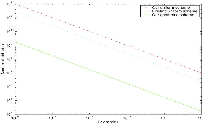
Figure 4. Comparison of Number of Grid Points ($\lambda=10^{3},\;d=500$)

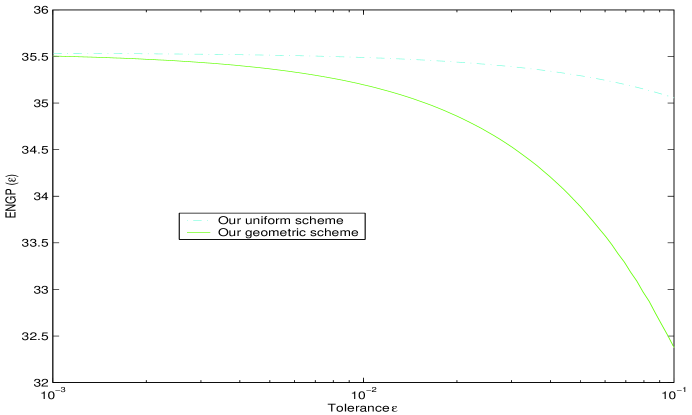
Figure 5. Comparison of $m_{eq}$ ($\lambda=10^{3},\;d=5,\;1+d\ln\lambda=35.5388$)

5. The Difficulties of Conventional Data Structure

Our previous sample reuse algorithm [6] uses the same data structure as that of the conventional algorithm. That is, the data structure for implementing the algorithms is basically a matrix of fixed size. In such data structure, for each grid point $r_{i}$, there is a record $(k_{i},n_{i})$ where $k_{i}$ represents the number of cases guaranteeing (or violating) the robustness requirement among $n_{i}$ simulations. In the course of experiment, the number $n_{i}$ is increment from $0$ to sample size $N$. In the following two subsections, we demonstrate that the conventional data structure is not suitable for controlling the error due to finite gridding.

5.1. The Issue of Data Processing

Clearly, the total number of records is exactly the number of grid points $m$. For the conventional method, to accomplish $N$ simulations for each grid points, the total number of updating the data record is $Nm$. As illustrated in Section 4, to control the error due to finite gridding requires an extremely large number, $m$, of grid points even for moderate requirement of $\epsilon$. Therefore, $Nm$ is usually a very large number. It can be shown that if the sample reuse algorithm employs the same data structure as that of the conventional method, then, for any gridding scheme with $m$ grid points, the total number of times of updating the data record is also $Nm$. This is true because, for every time a record $(k_{i},n_{i})$ is updated, the number $n_{i}$ can only be increased by $1$, and the number $n_{i}$ must be $N$ when the experiment is completed. To have a feeling that the data processing with the conventional data structure is a severe challenge, one can consider the example discussed in Remark 1 of Section 4. With $m\geq 3,240,000,001$ and normal sample size $10^{4}<N<10^{6}$, it can be seen that $Nm$ will be in the range of $3\times 10^{13}$ to $3\times 10^{15}$. This is an enormous burden for today’s computing technology. For a modern computer with $1.9$ GHz CPU and $256$ M bytes RAM, it takes about $20$ seconds to execute $10^{7}$ times the command $n_{i}\leftarrow n_{i}+1$ written in the MATLAB language. It can be reasonably inferred that updating the data record for $3\times 10^{13}$ times will take about $20\times 10^{-7}\times 3\times 10^{13}$ seconds (i.e., about $700$ days).

5.2. The Issue of Memory Space

For the conventional data structure, the total number of records is $m$. To execute the sample reuse algorithm or the conventional one with such data structure, each record must occupy some physical addresses. Such addresses are necessary for storing and visualizing the outcome of simulations. Of course, to obtain the outcome simulations may require a much higher amount of computer internal memory to execute the algorithm. Since $m$ is usually a very large number, the consumption of memory to store and visualize the output of simulation can be enormous. To illustrate, consider again the example discussed in Remark 1 of Section 4. Since a floating point number occupies $2$ bytes, storing a tuple of the form $(k_{i},n_{i})$ needs $4$ bytes. For $m\geq 3,240,000,001$, the data record will consumes $4\times 3,240,000,001\approx 13\times 10^{9}$ bytes (i.e., about $13$ giga bytes) of RAM. Such requirement, just for visualizing the outcome of the simulations, is a challenging task even for modern computers.

6. New Techniques of Sample Reuse

In the last section, we have shown that any algorithm using the conventional data structure suffer from the problems of the complexity of data processing and memory space. This is because, the sample size $N$ is usually very large and the number, $m$, of points in the partition of uncertainty radius approaches infinity as the tolerance, $\epsilon$, approaches zero (see Theorem 3). In this section, we shall demonstrate that, by introducing a dynamic data structure and a new sample reuse algorithm, the average requirement of memory and the computational effort devoted to data processing are absolutely bounded, independent of the tolerance, and well within the power of modern computers.

6.1. Data Structure

In order to address the memory issue and minimize the effort devoted to data processing, an appropriate data structure is critical. The key idea is to make use of the observation that, for a set of consecutive grid points with identical records of simulation results, it suffices to store the information of the smallest and the largest grid points. To illustrate our techniques, we enumerate, in a chronicle order of generation, the samples generated from various uncertainty bounding sets as $X_{1},X_{2},\cdots$. When samples $X_{1},X_{2},\cdots,X_{j}$ have been generated, the state of the experiment is completely represented by functions $\boldsymbol{s}(i,j)$ and $\boldsymbol{v}(i,j)$, where

$$\boldsymbol{s}(i,j)=\sum_{k=1}^{\boldsymbol{l}(i,j)}Y_{i}^{k},\qquad\boldsymbol{v}(i,j)=\sum_{k=1}^{\boldsymbol{l}(i,j)}Z_{i}^{k}$$

with

$$Y_{i}^{k}=\begin{cases}1&\text{if $X_{k}\in\mathcal{B}_{r_{i}}$};\\ 0&\text{otherwise}\end{cases}$$

(6.1) $$\boldsymbol{l}(i,j)=\max\left\{\ell:\;1\leq\ell\leq j,\;\sum_{k=1}^{\ell}Y_{i}^{k}\leq N\right\}$$

and

$$Z_{i}^{k}=\begin{cases}1&\text{if $X_{k}\in\mathcal{B}_{r_{i}}$ and $\mathbf{P}$ is violated for $X_{k}$};\\ 0&\text{otherwise}\end{cases}$$

for $i=1,\cdots,m$ and $k=1,\cdots,j$. The reason we introduce variable $\boldsymbol{l}(i,j)$ by (6.1) is that, for grid point $r_{i}$, once $N$ equivalent simulations are available, the subsequent simulations can be ignored. By the principle of sample reuse, $\boldsymbol{s}(i,j)$ and $\boldsymbol{v}(i,j)$ are, respectively, the accumulated numbers of samples and violations for uncertainty bounding set with radius $r_{i}$. When the experiment is completed, we have $\boldsymbol{n}$ samples $X_{1},X_{2},\cdots,X_{\boldsymbol{n}}$ and

$$\boldsymbol{s}(i,\boldsymbol{n})=N,\qquad\mathbb{P}(r_{i})=1-\frac{\boldsymbol{v}(i,\boldsymbol{n})}{N},\qquad i=1,\cdots,m.$$

It can be seen that $\boldsymbol{s}(i,j)$ is piece-wise constant (with respect to $i$) and there exists a matrix $S^{j}$ such that, for $i=1,\cdots,m$,

(6.2) $$\boldsymbol{s}(i,j)=\begin{cases}[S^{j}]_{\ell,2}&\text{for}\quad[S^{j}]_{\ell,1}\leq i<[S^{j}]_{\ell+1,1}\quad\text{with}\quad 1\leq\ell\leq\kappa-1;\\ [S^{j}]_{\kappa,2}&\text{for}\quad[S^{j}]_{\kappa,1}\leq i\leq m\end{cases}$$

where $\kappa$ is the number of rows of $S^{j}$ and $[A]_{\imath,\jmath}$ denotes the element of matrix $A$ in the $\imath$-th row and the $\jmath$-th column. Roughly speaking, the first column of matrix $S^{j}$ records the indexes of grid points for which the accumulated numbers of samples are jumping to different values. The second column of matrix $S^{j}$ records the corresponding accumulated numbers of samples.

Similarly, $\boldsymbol{v}(i,j)$ is piece-wise constant (with respect to $i$) and there exists a matrix $V^{j}$ such that, for $i=1,\cdots,m$,

(6.3) $$\boldsymbol{v}(i,j)=\begin{cases}[V^{j}]_{\ell,2}&\text{for}\quad[V^{j}]_{\ell,1}\leq i<[V^{j}]_{\ell+1,1}\quad\text{with}\quad 1\leq\ell\leq\tau-1;\\ [V^{j}]_{\tau,2}&\text{for}\quad[V^{j}]_{\tau,1}\leq i\leq m\end{cases}$$

where $\tau$ is the number of rows of $V^{j}$. Loosely speaking, the first column of matrix $V^{j}$ records the indexes of grid points for which the accumulated numbers of violations are jumping to different values. The second column of matrix $V^{j}$ records the corresponding accumulated numbers of violations.

In this paper, matrices $S^{j}$ and $V^{j}$ are, respectively, referred to as the matrix of sample sizes and the matrix of violations. At any stage that samples $X_{1},\cdots,X_{j}$ have been generated, the status of the experiment is completely characterized by matrices $S^{j},\;V^{j}$. Both matrices are of two columns but of varying number of rows in the course of experiment.

To save memory and data processing effort, we shall take advantage of the piece-wise constant property of the accumulated numbers of samples and violations. Hence, we shall construct matrices $S^{j}$ and $V^{j}$ when we have generated $X_{1},\cdots,X_{j}$. As can be seen in the sequel, such matrices can be constructed recursively. Once we have $S^{j}$ and $V^{j}$, we can generate sample $X_{j+1}$ and update $S^{j},\;V^{j}$ as $S^{j+1},\;V^{j+1}$ in accordance with equations (6.2) and (6.3).

6.2. Sample Reuse Algorithm

In this section, we present our sample reuse algorithms as follows.

Initialization:

We initialize the matrices of sample sizes and violations as follows:

$\quad\diamondsuit$ Generate sample $X_{1}$ uniformly from uncertainty set with radius $r_{m}$.

$\quad\diamondsuit$ Compute $\jmath$ such that $X_{1}\in\mathcal{B}_{r_{i}}$ for $\jmath\leq i\leq m$ and $X_{1}\notin\mathcal{B}_{r_{i}}$ for $1\leq i\leq\jmath-1$.

$\quad\diamondsuit$ Let $S^{1}=\begin{bmatrix}1&1\end{bmatrix}$ if $\jmath=1$ and $S^{1}=\begin{bmatrix}1&0\\ \jmath&1\end{bmatrix}$ if $\jmath>1$.

$\quad\diamondsuit$ Let $V^{1}=\begin{bmatrix}1&0\end{bmatrix}$ if $\mathbb{I}(X_{1})=0$ and $V^{1}=S^{1}$ if $\mathbb{I}(X_{1})=1$, where $\mathbb{I}(X)=1$ if the robustness requirement is violated for $X$ and otherwise $\mathbb{I}(X)=0$.

Sample generation:

If $[S^{j}]_{\kappa,1}<N$ then generate sample $X_{j+1}$ uniformly from uncertainty set with radius $r_{m}$, otherwise generate sample $X_{j+1}$ uniformly from uncertainty set with radius $[S^{j}]_{\kappa-1,1}$.

Updating matrices:

Update $S^{j}$ as $S^{j+1}$ by the method described in Section 6.2.1. If $\mathbb{I}(X_{j+1})=0$ then let $V^{j+1}=V^{j}$, otherwise update $V^{j}$ as $V^{j+1}$ by the method described in Section 6.2.2.

Stopping criterion:

The sampling process is terminated if $S^{j}$ has only one row and $[S^{j}]_{1,2}=N$.

6.2.1. Sample Sizes Tracking

In this section, we describe how to update the matrix of sample sizes. The key idea is to ensure condition (6.2). Let $\kappa$ be the number of rows of $S^{j}$. We proceed as follows.

Step (1):

Compute an index $\jmath^{*}$ such that $X_{j+1}\in\mathcal{B}_{r_{i}}$ for $\jmath^{*}\leq i\leq m$ and $X_{j+1}\notin\mathcal{B}_{r_{i}}$ for $1\leq i\leq\jmath^{*}-1$ (Note that explicit formulas for computing $\jmath^{*}$ are available when using uniform or geometric grid scheme).

Step (2):

Modify $S^{j}$ as a temporary matrix $\widehat{S}^{j+1}$ based on the following three cases.

Case (1): $[S^{j}]_{\ell^{*},1}<\jmath^{*}<[S^{j}]_{\ell^{*}+1,1}$ for some $\ell^{*}\in\{1,\cdots,\kappa-1\}$;

Case (2): $\jmath^{*}=[S^{j}]_{\ell^{*},1}$ for some $\ell^{*}\in\{1,\cdots,\kappa\}$;

Case (3): $\jmath^{*}>[S^{j}]_{\kappa,1}$.

In Case (1), define $\widehat{S}^{j+1}$ as a $(\kappa+1)\times 2$ matrix such that

$$\begin{array}[]{ll}[\widehat{S}^{j+1}]_{\ell,1}=[S^{j}]_{\ell,1},&\qquad[\widehat{S}^{j+1}]_{\ell,2}=[S^{j}]_{\ell,2},\quad\ell=1,\cdots,\ell^{*}\\ {[\widehat{S}^{j+1}]}_{\ell^{*}+1,1}=\jmath^{*},&\qquad[\widehat{S}^{j+1}]_{\ell^{*}+1,2}=1+[S^{j}]_{\ell^{*},2}\\ {[\widehat{S}^{j+1}]}_{\ell+1,1}=[S^{j}]_{\ell,1},&\qquad[\widehat{S}^{j+1}]_{\ell+1,2}=1+[S^{j}]_{\ell,2},\quad\ell=\ell^{*}+1,\cdots,\kappa.\end{array}$$

In Case (2), define $\widehat{S}^{j+1}$ as a $\kappa\times 2$ matrix such that

$$\begin{array}[]{ll}{[\widehat{S}^{j+1}]}_{\ell,1}=[S^{j}]_{\ell,1},&\qquad[\widehat{S}^{j+1}]_{\ell,2}=[S^{j}]_{\ell,2},\quad\ell=1,\cdots,\ell^{*}-1\\ {[\widehat{S}^{j+1}]}_{\ell,1}=[S^{j}]_{\ell,1},&\qquad[\widehat{S}^{j+1}]_{\ell,2}=1+[S^{j}]_{\ell,2},\quad\ell=\ell^{*},\cdots,\kappa.\end{array}$$

In Case (3), define $\widehat{S}^{j+1}$ as a $(\kappa+1)\times 2$ matrix such that

$$\begin{array}[]{ll}{[\widehat{S}^{j+1}]}_{\ell,1}=[S^{j}]_{\ell,1},&\qquad[\widehat{S}^{j+1}]_{\ell,2}=[S^{j}]_{\ell,2},\quad\ell=1,\cdots,\kappa\\ {[\widehat{S}^{j+1}]}_{\kappa+1,1}=\jmath^{*},&\qquad[\widehat{S}^{j+1}]_{\kappa+1,2}=1+[S^{j}]_{\kappa,2}.\end{array}$$

Step (3):

Let $\widehat{\kappa}$ denote the number of rows of $\widehat{S}^{j+1}$. If $[\widehat{S}^{j+1}]_{\widehat{\kappa},2}<N$ then let $S^{j+1}=\widehat{S}^{j+1}$, otherwise find index $\ell_{\star}$ by a bisection search such that $[\widehat{S}^{j}]_{\ell_{\star}-1,2}<N\leq[\widehat{S}^{j}]_{\ell_{\star},2}$ and define $S^{j+1}$ as an $\ell_{\star}\times 2$ matrix such that

$$\begin{array}[]{ll}{[S^{j+1}]}_{\ell,1}=[\widehat{S}^{j+1}]_{\ell,1},&\qquad[S^{j+1}]_{\ell,2}=[\widehat{S}^{j+1}]_{\ell,2},\quad\ell=1,\cdots,\ell_{\star}-1\\ {[S^{j+1}]}_{\ell_{\star},1}=[\widehat{S}^{j+1}]_{\ell_{\star},1},&\qquad[S^{j+1}]_{\ell_{\star},2}=[\widehat{S}^{j+1}]_{\ell_{\star},2}.\end{array}$$

6.2.2. Violations Tracking

In this section, we describe how to update the matrix of violations in the case of $\mathbb{I}(X_{j+1})=1$. The key idea is to ensure condition (6.3). Let $\kappa$ be the number of rows of $S^{j}$. Let $\tau$ be the number of rows of $V^{j}$. Let $\jmath^{*}$ be the index obtained in the process of updating $S^{j}$ such that $X_{j+1}\in\mathcal{B}_{r_{i}}$ for $\jmath^{*}\leq i\leq m$ and $X_{j+1}\notin\mathcal{B}_{r_{i}}$ for $1\leq i\leq\jmath^{*}-1$. We proceed as follows.

Step (i):

Identify the maximal index $\iota$ such that the experiment for uncertainty radius $r_{\iota}$ has not been completed by the following method.

$\diamondsuit$ If $[S^{j}]_{\kappa,2}<N$, then let $\iota=\kappa$, otherwise find $\iota$ by a bisection search such that $[V^{j}]_{\iota,1}<[S^{j}]_{\kappa,1},\quad[V^{j}]_{\iota+1,1}\geq[S^{j}]_{\kappa,1}$.

Step (ii):

Modify $V^{j}$ as a temporary matrix $\widehat{V}^{j}$ based on the following two cases.

Case(a) : $[S^{j}]_{\kappa,2}<N$ or $[S^{j}]_{\kappa,2}=N,\quad[V^{j}]_{\iota+1,1}=[S^{j}]_{\kappa,1}$.

Case(b) : $[S^{j}]_{\kappa,2}\geq N$ and the index $\iota$ guarantees $[V^{j}]_{\iota+1,1}>[S^{j}]_{\kappa,1}$.

In Case (a), we define $\widehat{V}^{j}=V^{j}$. In Case (b), we define $\widehat{V}^{j}$ as a $(\tau+1)\times 2$ matrix such that

$$\begin{array}[]{ll}{[\widehat{V}^{j}]}_{\ell,1}=[V^{j}]_{\ell,1},&\qquad[\widehat{V}^{j}]_{\ell,2}=[V^{j}]_{\ell,2},\quad\ell=1,\cdots,\iota\\ {[\widehat{V}^{j}]}_{\iota+1,1}=[S^{j}]_{\kappa,1},&\qquad[\widehat{V}^{j}]_{\iota+1,2}=[V^{j}]_{\iota,2}\\ {[\widehat{V}^{j}]}_{\ell+1,1}=[V^{j}]_{\ell,1},&\qquad[\widehat{V}^{j}]_{\ell+1,2}=[V^{j}]_{\ell,2},\quad\ell=\iota+1,\cdots,\tau.\end{array}$$

Step (iii):

Obtain $V^{j+1}$ by modifying $\widehat{V}^{j}$ based on the following three cases.

Case (i): $[\widehat{V}^{j}]_{\ell^{*},1}<\jmath^{*}<[\widehat{V}^{j}]_{\ell^{*}+1,1}$ for some $\ell^{*}\in\{1,\cdots,\iota-1\}$;

Case (ii): $\jmath^{*}=[\widehat{V}^{j}]_{\ell^{*},1}$ for some $\ell^{*}\in\{1,\cdots,\iota\}$;

Case (iii): $\jmath^{*}>[\widehat{V}^{j}]_{\iota,1}$.

Let $\widehat{\tau}$ be the number of rows of $\widehat{V}^{j}$. In Case (i), define $V^{j+1}$ as a $(\widehat{\tau}+1)\times 2$ matrix such that

$$\begin{array}[]{ll}{[V^{j+1}]}_{\ell,1}=[\widehat{V}^{j}]_{\ell,1},&\qquad[V^{j+1}]_{\ell,2}=[\widehat{V}^{j}]_{\ell,2},\quad\ell=1,\cdots,\ell^{*}\\ {[V^{j+1}]}_{\ell^{*}+1,1}=\jmath^{*},&\qquad[V^{j+1}]_{\ell^{*}+1,2}=1+[\widehat{V}^{j}]_{\ell^{*},2}\\ {[V^{j+1}]}_{\ell+1,1}=[\widehat{V}^{j}]_{\ell,1},&\qquad[V^{j+1}]_{\ell+1,2}=1+[\widehat{V}^{j}]_{\ell,2},\quad\ell=\ell^{*}+1,\cdots,\iota\\ {[V^{j+1}]}_{\ell+1,1}=[\widehat{V}^{j}]_{\ell,1},&\qquad[V^{j+1}]_{\ell+1,2}=[\widehat{V}^{j}]_{\ell,2},\quad\ell=\iota+1,\cdots,\widehat{\tau}.\end{array}$$

In Case (ii), define $V^{j+1}$ as a $\widehat{\tau}\times 2$ matrix such that

$$\begin{array}[]{ll}{[V^{j+1}]}_{\ell,1}=[\widehat{V}^{j}]_{\ell,1},&\qquad[V^{j+1}]_{\ell,2}=[\widehat{V}^{j}]_{\ell,2},\quad\ell=1,\cdots,\ell^{*}-1\\ {[V^{j+1}]}_{\ell,1}=[\widehat{V}^{j}]_{\ell,1},&\qquad[V^{j+1}]_{\ell,2}=1+[\widehat{V}^{j}]_{\ell,2},\quad\ell=\ell^{*},\cdots,\iota\\ {[V^{j+1}]}_{\ell,1}=[\widehat{V}^{j}]_{\ell,1},&\qquad[V^{j+1}]_{\ell,2}=[\widehat{V}^{j}]_{\ell,2},\quad\ell=\iota+1,\cdots,\widehat{\tau}.\end{array}$$

In Case (iii), define $V^{j+1}$ as a $(\widehat{\tau}+1)\times 2$ matrix such that

$$\begin{array}[]{ll}{[V^{j+1}]}_{\ell,1}=[\widehat{V}^{j}]_{\ell,1},&\qquad[V^{j+1}]_{\ell,2}=[\widehat{V}^{j}]_{\ell,2},\quad\ell=1,\cdots,\iota\\ {[V^{j+1}]}_{\iota+1,1}=\jmath^{*},&\qquad[V^{j+1}]_{\iota+1,2}=1+[\widehat{V}^{j}]_{\iota,2}\\ {[V^{j+1}]}_{\ell+1,1}=[\widehat{V}^{j}]_{\ell,1},&\qquad[V^{j+1}]_{\ell+1,2}=[\widehat{V}^{j}]_{\ell,2},\quad\ell=\iota+1,\cdots,\widehat{\tau}.\end{array}$$

6.3. Complexity of Data Processing and Memory

It can be seen that the memory requirement and the computation due to data processing are determined by the sizes of matrices $S^{j}$ and $V^{j}$. To quantify the complexity, we have the following results.

Theorem 5.

For any $j$, the following statements hold true:

(I):

The number of rows of matrix $S^{j}$ is no more than $N$;

(II):

The expected number of rows of matrix $V^{j}$ is no greater than

(6.4) $$1+N\left[P_{e}(a)+2d\int_{\frac{a}{\hbar}}^{a}\frac{P_{e}(x)}{x}dx\right]\leq 1+NP_{e}(a)\left(1+2d\ln\hbar\right)$$

where $P_{e}(x)=1-\min_{y\in[\frac{a}{\lambda},\;x]}\mathbb{P}(y),\;\forall x\in\left[\frac{a}{\lambda},\;a\right]$ and

$$\hbar=\max\left(\min\left(\lambda,\frac{a}{\rho_{0}}\right),\;1\right)$$

with $\rho_{0}=\sup\{r\mid\mathbb{P}(r)=1\}$.

See Appendix F for a proof. We now revisit the robustness analysis problem discussed in Remark 1 of Section 4 from the perspective of memory complexity. Assume that each data record $(k_{i},n_{i})$ (or each row of $V^{j}$) occupies $4$ bytes of computer internal memory (RAM). As illustrated in Section $5.2$, when using the conventional data structure, it takes $13$G (giga bytes) of RAM to save the data and visualize the results. On the other hand, in our new algorithm, if the smallest proportion is $p_{*}=\min_{r\in\left[\frac{a}{\lambda},a\right]}\mathbb{P}(r)>0.999$ and $\hbar<\frac{3}{2}$, the RAM requirement will be equivalent to

$$4\times\left[1+(1-p_{*})\left(1+2d\ln\hbar\right)N\right]$$

$$= 4\times\left[1+(1-0.999)\times\left(1+2\times 1800\times\ln\frac{3}{2}\right)\times 10^{6}\right]$$

$$< 6.2\times 10^{6}\;\text{bytes}\approx 6.2\;\text{M}\;\text{bytes}.$$

It can be seen that such requirement of memory is extremely low as compared to that of the conventional method. Theorem 5 also reveals that the complexity of data processing is very low.

6.4. Confidence Band

To be useful, any numerical techniques should provide a method for error assessment. Monte Carlo simulation is no exception. The following results allows us to construct confidence band for the robustness curve. Such post-experimental statistical inference can remedy the conservatism of a priori choice of sample size $N$ based on the Chernoff bound. In order to overcome the computational complexity of the Clopper-Pearson’s confidence interval [9], we have developed new methods to facilitate the construction of the confidence band.

Theorem 6.

Let $\delta\in(0,1)$. Let $\mathcal{L}(k)=\frac{k}{N}+\frac{3}{4}\;\frac{1-\frac{2k}{N}-\sqrt{1+4\theta\;k(1-\frac{k}{N})}}{1+\theta N}$ and $\mathcal{U}(k)=\frac{k}{N}+\frac{3}{4}\;\frac{1-\frac{2k}{N}+\sqrt{1+4\theta\;k(1-\frac{k}{N})}}{1+\theta N}$ with $\theta=\frac{9}{8\ln\frac{2}{\delta}}$. Let $\zeta=\frac{r-r_{i}}{r_{i+1}-r_{i}}$. Let

$$K_{i}=N-\boldsymbol{v}(i,\boldsymbol{n}),\qquad i=1,\cdots,m.$$

Let $\varsigma=1-\frac{g(r_{\star})}{r_{i+1}-r_{i}}$. Define $\overline{\mathbb{P}}(r)=\zeta\;\mathcal{U}(K_{i})+(1-\zeta)\;\mathcal{U}(K_{i+1})+\varsigma$ and $\underline{\mathbb{P}}(r)=\zeta\;\mathcal{L}(K_{i})+(1-\zeta)\;\mathcal{L}(K_{i+1})-\varsigma$. Then

$$\Pr\{\underline{\mathbb{P}}(r)<\mathbb{P}(r)<\overline{\mathbb{P}}(r),\;\forall r\in[r_{i},r_{i+1}]\}>1-\delta.$$

See Appendix G for a proof. The family of intervals $[\underline{\mathbb{P}}(r),\;\overline{\mathbb{P}}(r)],\;r\in[a/\lambda,\;a]$ is referred to as the confidence band. It is important to note that the confidence band can be efficiently constructed by making use of the piece-wise constant property of $\boldsymbol{v}(i,\boldsymbol{n})$. It can be shown that the computational complexity of constructing the confidence band is also absolutely bounded.

7. Conclusion

It is possible to make a case for the statement that the probabilistic robustness analysis is essentially the study of the robustness function, especially about its probabilistic implications, efficient evaluation and computational complexity. We have addressed these issues in this paper. In particular, we have developed randomized algorithms which offer more insights for system robustness. We rigorously show that, in both aspects of computer running time and memory requirement, the complexity of such randomized algorithms is not only linear in the dimension of uncertainty space, but also surprisingly low. While the complexity of conventional method grows linearly with the number of grid points and the error due to interpolation is not well controlled, our techniques completely resolve such issues. In short, our method guarantees accuracy and efficiency.

Appendix A Proof of Theorem 1

We first establish a basic inequality that will be used to prove the theorem.

Lemma 1.

For any $x>1$,

$$\frac{1}{x}+\ln x>1.$$

Proof. Let

$$f(x)=\frac{1}{x}+\ln x.$$

Then $f(1)=1$ and

$$\frac{d\;f(x)}{dx}=\frac{x-1}{x^{2}}>0,\qquad\forall x>1.$$

It follows that $f(x)>1,\;\forall x>1$. $\Box$

Now we are in the position to prove Theorem 1. Observing that

$$\left(\frac{r_{m}}{r_{1}}\right)^{d}=\prod_{i=1}^{m-1}\left(\frac{r_{i+1}}{r_{i}}\right)^{d},$$

we have

$$\ln\left(\frac{r_{m}}{r_{1}}\right)^{d}=\sum_{i=1}^{m-1}\ln\left(\frac{r_{i+1}}{r_{i}}\right)^{d}.$$

Therefore,

$$\sum_{i=1}^{m-1}\left(\frac{r_{i}}{r_{i+1}}\right)^{d}+\ln\left(\frac{r_{m}}{r_{1}}\right)^{d} = \sum_{i=1}^{m-1}\left[\frac{1}{\left(\frac{r_{i+1}}{r_{i}}\right)^{d}}+\ln\left(\frac{r_{i+1}}{r_{i}}\right)^{d}\right].$$

Since $\left(\frac{r_{i+1}}{r_{i}}\right)^{d}>1,\;i=1,\cdots,m-1$, it follows from Lemma 1 that

$$\frac{1}{\left(\frac{r_{i+1}}{r_{i}}\right)^{d}}+\ln\left(\frac{r_{i+1}}{r_{i}}\right)^{d}>1,\qquad i=1,\cdots,m-1.$$

Hence,

$$\sum_{i=1}^{m-1}\left(\frac{r_{i}}{r_{i+1}}\right)^{d}+\ln\left(\frac{r_{m}}{r_{1}}\right)^{d}>m-1,$$

or equivalently,

$$m-\sum_{i=1}^{m-1}\left(\frac{r_{i}}{r_{i+1}}\right)^{d}<1+\ln\left(\frac{r_{m}}{r_{1}}\right)^{d}=1+d\ln\lambda.$$

Finally, by Theorem 1 of [6] and the definition of $m_{\mathrm{eq}}$, we have

$$m_{\mathrm{eq}}=m-\sum_{i=1}^{m-1}\left(\frac{r_{i}}{r_{i+1}}\right)^{d}<1+d\ln\lambda.$$

Appendix B Proof of Theorem 2

To prove the theorem, we need some preliminary results. It is derived in [2] that $\left|\frac{d\mathbb{P}(r)}{dr}\right|<\frac{2d}{r}$ when $\mathbb{P}(.)$ is differentiable. The following lemma indicates that the bound on the rate of variation of $\mathbb{P}(.)$ can be much tighter.

Lemma 2.

For arbitrary robustness requirement,

$$\left|\mathbb{P}(r+\varDelta r)-\mathbb{P}(r)\right|\leq 1-\left(1+\frac{\varDelta r}{r}\right)^{-d}<\frac{d}{r}\;\varDelta r$$

for any $r>0$ and any $\varDelta r>0$.

Proof.

Let $\mathcal{Q}_{r}\subseteq\mathcal{B}_{r}$ be the set such that the robustness requirement is satisfied. Let

$$I_{1}=\frac{\text{vol}(\mathcal{Q}_{r+\varDelta r})}{\text{vol}(\mathcal{B}_{r+\varDelta r})}-\frac{\text{vol}(\mathcal{Q}_{r})}{\text{vol}(\mathcal{B}_{r+\varDelta r})},\qquad I_{2}=\frac{\text{vol}(\mathcal{Q}_{r})}{\text{vol}(\mathcal{B}_{r+\varDelta r})}-\frac{\text{vol}(\mathcal{Q}_{r})}{\text{vol}(\mathcal{B}_{r})}.$$

Let “$\setminus$” denote the operation of set minus. Observing that $\mathcal{Q}_{r+\varDelta r}\setminus\mathcal{Q}_{r}\subseteq\mathcal{B}_{r+\varDelta r}\setminus\mathcal{B}_{r}$, we have $\text{vol}(\mathcal{Q}_{r+\varDelta r})-\text{vol}(\mathcal{Q}_{r})\leq\text{vol}(\mathcal{B}_{r+\varDelta r})-\text{vol}(\mathcal{B}_{r})$. Using this fact and the identity $\text{vol}(\mathcal{B}_{r})=r^{d}\;\text{vol}(\mathcal{B}_{1})$, we have

$$0\leq I_{1}\leq\frac{\text{vol}(\mathcal{B}_{r+\varDelta r})-\text{vol}(\mathcal{B}_{r})}{\text{vol}(\mathcal{B}_{r+\varDelta r})}=1-\left(1+\frac{\varDelta r}{r}\right)^{-d}$$

and

$$-\left[1-\left(1+\frac{\varDelta r}{r}\right)^{-d}\right]\leq-\frac{\text{vol}(\mathcal{Q}_{r})}{\text{vol}(\mathcal{B}_{r})}\frac{\text{vol}(\mathcal{B}_{r+\varDelta r})-\text{vol}(\mathcal{B}_{r})}{\text{vol}(\mathcal{B}_{r+\varDelta r})}=I_{2}\leq 0.$$

Therefore, $\left|\mathbb{P}(r+\varDelta r)-\mathbb{P}(r)\right|=|I_{1}+I_{2}|\leq 1-\left(1+\frac{\varDelta r}{r}\right)^{-d}<\frac{d}{r}\varDelta r$ where the last inequality follows from inequality $1-\left(1+\frac{x}{r}\right)^{-d}<\frac{dx}{r},\;\forall x>0$. To prove this inequality, we can define function $h(x)\stackrel{{\scriptstyle\mathrm{def}}}{{=}}1-\left(1+\frac{x}{r}\right)^{-d}-\frac{dx}{r},\;x>0$ and check that $h(0)=0$ and $\frac{\partial h(x)}{\partial x}=\frac{d}{r}\left[\left(1+\frac{x}{r}\right)^{-(d+1)}-1\right]<0,\;\forall x>0$.

$\Box$

We are now in the position to prove the theorem. It can be shown that

(B.1) $$|\mathbb{P}(r)-\mathbb{P}^{*}(r)| = \left|\frac{(r_{i+1}-r)[\mathbb{P}(r)-\mathbb{P}(r_{i})]+(r-r_{i})[\mathbb{P}(r)-\mathbb{P}(r_{i+1})]}{r_{i+1}-r_{i}}\right|$$

$$\leq \frac{(r_{i+1}-r)|\mathbb{P}(r)-\mathbb{P}(r_{i})|+(r-r_{i})|\mathbb{P}(r)-\mathbb{P}(r_{i+1})|}{r_{i+1}-r_{i}}.$$

By Lemma 2 and inequality (B.1), we have

$$|\mathbb{P}(r)-\mathbb{P}^{*}(r)| \leq \frac{(r_{i+1}-r)\left[1-\left(\frac{r}{r_{i}}\right)^{-d}\right]+(r-r_{i})\left[1-\left(\frac{r_{i+1}}{r}\right)^{-d}\right]}{r_{i+1}-r_{i}}$$

$$= 1-\frac{g(r)}{r_{i+1}-r_{i}}.$$

Note that

$$\frac{\partial g(r)}{\partial r}=\Phi(r)-\Psi(r)$$

where

$$\Phi(r)=\left(\frac{r_{i+1}}{r}\right)^{-d}\left[1+\left(1-\frac{r_{i}}{r}\right)d\right],\qquad\Psi(r)=\left(\frac{r}{r_{i}}\right)^{-d}\left[1+\left(\frac{r_{i+1}}{r}-1\right)d\right].$$

It can be verified that

$$\Phi(r_{i})=\left(\frac{r_{i+1}}{r_{i}}\right)^{-d}<1,\qquad\Psi(r_{i})=1+\left(\frac{r_{i+1}}{r_{i}}-1\right)d>1,\qquad\left.\frac{\partial g(r)}{\partial r}\right|_{r=r_{i}}<0,$$

$$\Phi(r_{i+1})=1+\left(1-\frac{r_{i}}{r_{i+1}}\right)d>1,\quad\Psi(r_{i+1})=\left(\frac{r_{i+1}}{r_{i}}\right)^{-d}<1,\quad\left.\frac{\partial g(r)}{\partial r}\right|_{r=r_{i+1}}>0.$$

It can be checked that $\Phi(r)$ is a monotone increasing function of $r$ and that $\Psi(r)$ is a monotone decreasing function of $r$. Hence, $\frac{\partial g(r)}{\partial r}$ is a monotone increasing function of $r$. Moreover, there exists an unique $r_{\star}\in(r_{i},\;r_{i+1})$ such that $\left.\frac{\partial g(r)}{\partial r}\right|_{r=r_{\star}}=0$, i.e., $\Phi(r_{\star})=\Psi(r_{\star})$. Furthermore, $g(r)$ is a convex function of $r$. Consequently,

$$\min_{r\in[r_{i},\;r_{i+1}]}g(r)=g(r_{\star})$$

and we have shown

$$|\mathbb{P}(r)-\mathbb{P}^{*}(r)|\leq 1-\frac{g(r_{\star})}{r_{i+1}-r_{i}}\qquad\forall r\in[r_{i},\;r_{i+1}].$$

Since $\frac{\partial g(r)}{\partial r}$ is a monotone increasing function of $r$, we can compute $r_{\star}$ by a bisection search over interval $(r_{i},\;r_{i+1})$.

By Lemma 2 and inequality (B.1), we have

$$|\mathbb{P}(r)-\mathbb{P}^{*}(r)| \leq \frac{(r_{i+1}-r)(r-r_{i})\frac{d}{r_{i}}+(r-r_{i})(r_{i+1}-r)\frac{d}{r}}{r_{i+1}-r_{i}}$$

$$\leq \frac{(r_{i+1}-r)(r-r_{i})\frac{d}{r_{i}}+(r-r_{i})(r_{i+1}-r)\frac{d}{r_{i}}}{r_{i+1}-r_{i}}$$

$$\leq \frac{2d}{r_{i}(r_{i+1}-r_{i})}\;\max_{r\in[r_{i},r_{i+1}]}(r_{i+1}-r)(r-r_{i})$$

$$= \frac{2d}{r_{i}(r_{i+1}-r_{i})}\;\frac{(r_{i+1}-r_{i})^{2}}{4}$$

$$= \frac{d(r_{i+1}-r_{i})}{2r_{i}}.$$

Appendix C Proof of Theorem 3

By Theorem 2, $|\mathbb{P}(r)-\mathbb{P}^{*}(r)|\leq\frac{d\;(r_{i+1}-r_{i})}{2r_{i}},\quad\forall r\in[r_{i},r_{i+1}]$. Thus, it suffices to show $\frac{d\;(r_{i+1}-r_{i})}{2r_{i}}<\epsilon$, i.e.,

(C.1) $$\frac{r_{i+1}}{r_{i}}<1+\frac{2\epsilon}{d}.$$

By definition (4.1), for $i=1,\cdots,m-1$,

$$\frac{r_{i+1}}{r_{i}} = \frac{a-\frac{(m-i-1)(\lambda-1)}{(m-1)\lambda}a}{a-\frac{(m-i)(\lambda-1)}{(m-1)\lambda}a}$$

$$= 1+\frac{\lambda-1}{m-1+(\lambda-1)(i-1)}$$

$$\leq 1+\frac{\lambda-1}{m-1}.$$

By virtue of (C.1), to guarantee that the gridding error is less than $\epsilon$, it suffices to ensure $1+\frac{\lambda-1}{m-1}<1+\frac{2\epsilon}{d}$, i.e., $m>1+\frac{d(\lambda-1)}{2\epsilon}$. Hence, it suffices to have

$$m\geq 2+\left\lfloor\frac{(\lambda-1)d}{2\epsilon}\right\rfloor.$$

It can be verified that

$$\frac{r_{i}}{r_{i+1}}=1-\frac{1}{\frac{m-1}{\lambda-1}+i},\qquad i=1,\cdots,m-1.$$

By Theorem 1 of [6], the sample reuse factor is given by

$$\mathcal{F}_{\mathrm{reuse}} = \frac{m}{m-\sum_{i=1}^{m-1}\left(\frac{r_{i}}{r_{i+1}}\right)^{d}}$$

$$= \frac{m}{m-\sum_{i=1}^{m-1}\left(1-\frac{1}{\frac{m-1}{\lambda-1}+i}\right)^{d}}.$$

Therefore,

$$m_{\mathrm{eq}}(\epsilon)=\frac{m}{\mathcal{F}_{\mathrm{reuse}}}=m-\sum_{i=1}^{m-1}\left(1-\frac{1}{\frac{m-1}{\lambda-1}+i}\right)^{d}.$$

Appendix D Proof of Theorem 4

By virtue of (4.2), we have $\frac{r_{i+1}}{r_{i}}=\lambda^{\frac{1}{m-1}}$. Hence, by (C.1), it suffices to show $\lambda^{\frac{1}{m-1}}<1+\frac{2\epsilon}{d}$, which can be reduced to $m>1+\frac{\ln\lambda}{\ln\left(1+\frac{2\epsilon}{d}\right)}$. This inequality is equivalent to $m\geq 2+\left\lfloor\frac{\ln\lambda}{\ln\left(1+\frac{2\epsilon}{d}\right)}\right\rfloor$. By equation (3.1) and Theorem 1 of [6], we have $\mathbb{E}[\boldsymbol{n}]=\left[m-(m-1)\left(\frac{1}{\lambda}\right)^{\frac{d}{m-1}}\right]N$ and hence obtain $m_{\mathrm{eq}}(\epsilon)$. Note that

$$\mathcal{F}_{\mathrm{reuse}}=\frac{m}{m_{\mathrm{eq}}(\epsilon)}>\frac{m}{1+d\;\ln\lambda}=\frac{2+\left\lfloor\frac{\ln\lambda}{\ln\left(1+\frac{2\epsilon}{d}\right)}\right\rfloor}{1+d\;\ln\lambda}>\frac{\frac{\ln\lambda}{\ln\left(1+\frac{2\epsilon}{d}\right)}}{1+d\;\ln\lambda}.$$

Making use of the inequality $\ln(1+x)<x,\;\forall x>0$, we have $\ln\left(1+\frac{2\epsilon}{d}\right)<\frac{2\epsilon}{d}$. Therefore,

$$\mathcal{F}_{\mathrm{reuse}}>\frac{\frac{\ln\lambda}{\frac{2\epsilon}{d}}}{1+d\;\ln\lambda}\\ =\frac{1}{2\epsilon}\left(1-\frac{1}{1+d\;\ln\lambda}\right).$$

Appendix E Proof of Theorem 5

Proof of statement (I):

Obviously, $[S^{j}]_{1,2}\geq 1,\quad[S^{j}]_{\kappa,2}\leq N$. From the rules of sampling, we can perform induction with respect to $j$ and have $[S^{j}]_{\ell+1,2}-[S^{j}]_{\ell,2}\geq 1,\;\ell=1,\cdots,\kappa-1$. Observing that

$$[S^{j}]_{\kappa,2} = [S^{j}]_{1,2}+\sum_{\ell=1}^{\kappa-1}\left([S^{j}]_{\ell+1,2}-[S^{j}]_{\ell,2}\right)$$

$$\geq 1+\sum_{\ell=1}^{\kappa-1}\left([S^{j}]_{\ell+1,2}-[S^{j}]_{\ell,2}\right)$$

$$\geq 1+\kappa-1$$

$$= \kappa,$$

we have $\kappa\leq[S^{j}]_{\kappa,2}\leq N$.

Proof of statement (II):

We need some preliminary results.

Lemma 3.

Let $1\leq i\leq m-1$. Then

$$\left|\left[1-\left(\frac{r_{i}}{r_{i+1}}\right)^{d}\right]-\frac{d(r_{i+1}-r_{i})}{r_{i+1}}\right|\leq\frac{d(d-1)}{2}\;\left(\frac{r_{i+1}-r_{i}}{r_{i+1}}\right)^{2}.$$

Proof.

Note that

$$\left|\left[1-\left(\frac{r_{i}}{r_{i+1}}\right)^{d}\right]-\frac{d(r_{i+1}-r_{i})}{r_{i+1}}\right| = \left|\left(\frac{r_{i}}{r_{i+1}}\right)^{d}-\left(1-\frac{d(r_{i+1}-r_{i})}{r_{i+1}}\right)\right|$$

$$= \left|\left(1-t\right)^{d}-\left(1-d\;t\right)\right|$$

where $t=\frac{r_{i+1}-r_{i}}{r_{i+1}}$. It can be checked that $\left|\left(1-t\right)^{d}-\left(1-d\;t\right)\right|=\frac{d(d-1)}{2}t^{2}$ for $d=1,2$. For $d\geq 3$, by Taylor’s expansion formula, there exists $\xi\in(0,t)$ such that

$$(1-t)^{d}=1-d\;t+\frac{d(d-1)}{2}(1-\xi)^{d-2}\;t^{2}.$$

Observing that $0<t<1$ since $0<r_{i}<r_{i+1}$, we hence have $0<(1-\xi)^{d-2}<1$ and $\left|\left(1-t\right)^{d}-\left(1-d\;t\right)\right|<\frac{d(d-1)}{2}t^{2}$ for $d\geq 3$. Therefore, for any $d\geq 1$,

$$\left|\left[1-\left(\frac{r_{i}}{r_{i+1}}\right)^{d}\right]-\frac{d(r_{i+1}-r_{i})}{r_{i+1}}\right|\leq\frac{d(d-1)}{2}t^{2}=\frac{d(d-1)}{2}\;\left(\frac{r_{i+1}-r_{i}}{r_{i+1}}\right)^{2}.$$

$\Box$

Lemma 4.

Define the maximum gap between grid points as

$$\varpi=\max_{1\leq i\leq m-1}\;(r_{i+1}-r_{i}).$$

Then

$$\sum_{i=1}^{m-1}\left(\frac{r_{i+1}-r_{i}}{r_{i+1}}\right)^{2}<\frac{\lambda(\lambda-1)\varpi}{a}.$$

Proof.

Note that

$$\sum_{i=1}^{m-1}\left(\frac{r_{i+1}-r_{i}}{r_{i+1}}\right)^{2}\leq\varpi\sum_{i=1}^{m-1}\frac{r_{i+1}-r_{i}}{r_{i+1}^{2}}<\varpi\sum_{i=1}^{m-1}\frac{r_{i+1}-r_{i}}{\left(\frac{a}{\lambda}\right)^{2}}.$$

By successive cancelation,

$$\sum_{i=1}^{m-1}(r_{i+1}-r_{i})=r_{m}-r_{1}=a-\frac{a}{\lambda}.$$

Hence,

$$\sum_{i=1}^{m-1}\left(\frac{r_{i+1}-r_{i}}{r_{i+1}}\right)^{2}<\varpi\sum_{i=1}^{m-1}\frac{r_{i+1}-r_{i}}{\left(\frac{a}{\lambda}\right)^{2}}=\varpi\;\frac{a-\frac{a}{\lambda}}{\left(\frac{a}{\lambda}\right)^{2}}=\frac{\lambda(\lambda-1)\varpi}{a}.$$

$\Box$

Lemma 5.

The expected number of rows of the matrix of violations $V^{\boldsymbol{n}}$ is no greater than $1+NP_{e}(a)+2N\sum_{j=1}^{m-1}P_{e}(r_{j})\left[1-\left(\frac{r_{j}}{r_{j+1}}\right)^{d}\right]$.

Proof.

Let $X_{1}^{j},\cdots,X_{\mathbf{n}_{j}}^{j}$ be the samples generated from uncertainty set with radius $r_{j}$. Let $Y_{i}^{j}=\mathbb{I}(X_{i}^{j}),\quad i=1,\cdots,\mathbf{n}_{j}$. By the principle of sample reuse, the value of $\mathbf{n}_{j}$ depends only on the samples generated from uncertainty sets with radius $r_{k},\;j+1\leq k\leq m$. Consequently, event $\{\mathbf{n}_{j}=\nu\}$ is independent of event $\{Y_{i}^{j}=1\}$ and $\Pr\{Y_{i}^{j}=1,\;\mathbf{n}_{j}=\nu\}=\Pr\{Y_{i}^{j}=1\}\Pr\{\mathbf{n}_{j}=\nu\}$. By the definitions of $Y_{i}^{j}$ and $P_{e}(.)$, we have $\Pr\{Y_{i}^{j}=1\}=1-\mathbb{P}(r_{j})\leq P_{e}(r_{j})$. Therefore,

$$\mathbb{E}\left[\sum_{i=1}^{\mathbf{n}_{j}}Y_{i}^{j}\right] = \sum_{\nu=1}^{N}\sum_{i=1}^{\nu}\Pr\{Y_{i}^{j}=1,\;\mathbf{n}_{j}=\nu\}$$

$$= \sum_{\nu=1}^{N}\sum_{i=1}^{\nu}\Pr\{Y_{i}^{j}=1\}\Pr\{\mathbf{n}_{j}=\nu\}$$

$$\leq \sum_{\nu=1}^{N}\nu\;P_{e}(r_{j})\Pr\{\mathbf{n}_{j}=\nu\}$$

$$= P_{e}(r_{j})\;\mathbb{E}[\mathbf{n}_{j}]$$

for $j=1,\cdots,m$. We now consider $V^{\boldsymbol{n}}$ with $\boldsymbol{n}=\sum_{i=1}^{m}\mathbf{n}_{i}$. By the mechanism of the sample reuse algorithms, for $j=1,\cdots,m-1$, every new sample from uncertainty set with radius $r_{j}$ at most creates $2Y_{i}^{j},\;i=1,\cdots,\mathbf{n}_{j}$ new rows for the matrix of violations (see Section $6.2.2$). Note that $X_{1}$ create at most $1+Y_{1}^{m}$ rows for $V^{1}$. Every new sample from uncertainty set with radius $r_{m}$ at most creates $Y_{i}^{m},\;i=2,\cdots,\mathbf{n}_{m}$ new rows for the matrix of violations. Hence

$$\mathbb{E}[\text{The number of rows of matrix $V^{\boldsymbol{n}}$}]$$

$$\leq 1+\mathbb{E}\left[\sum_{i=1}^{\mathbf{n}_{m}}Y_{i}^{m}\right]+2\;\mathbb{E}\left[\sum_{j=1}^{m-1}\sum_{i=1}^{\mathbf{n}_{j}}Y_{i}^{j}\right]$$

$$\leq 1+P_{e}(r_{m})\;\mathbb{E}[\mathbf{n}_{m}]+2\sum_{j=1}^{m-1}P_{e}(r_{j})\;\mathbb{E}[\mathbf{n}_{j}].$$

By Lemma 6 of [6], we have

(E.1) $$\mathbb{E}[\mathbf{n}_{j}]=\left[1-\left(\frac{r_{j}}{r_{j+1}}\right)^{d}\right]N,\qquad j=1,\cdots,m-1.$$

By (E.1) and using the fact that $\mathbb{E}[\mathbf{n}_{m}]=N,\;P_{e}(r_{m})=P_{e}(a)$, we have

$$\mathbb{E}[\text{The number of rows of matrix $V^{\boldsymbol{n}}$}]\leq 1+NP_{e}(a)+2N\sum_{j=1}^{m-1}P_{e}(r_{j})\left[1-\left(\frac{r_{j}}{r_{j+1}}\right)^{d}\right].$$

$\Box$

Lemma 6.

For any grid scheme,

$$\left|\sum_{i=1}^{m-1}P_{e}(r_{i})\left[1-\left(\frac{r_{i}}{r_{i+1}}\right)^{d}\right]-d\sum_{i=1}^{m-1}\frac{P_{e}(r_{i+1})(r_{i+1}-r_{i})}{r_{i+1}}\right|$$

$$< \frac{d(d-1)\lambda(\lambda-1)\varpi}{2a}+\frac{\lambda d}{a}\;\sum_{i=1}^{m-1}P_{e}(r_{i+1})(r_{i+1}-r_{i})-\frac{\lambda d}{a}\;\sum_{i=1}^{m-1}P_{e}(r_{i})(r_{i+1}-r_{i}).$$

Proof.

Note that

$$\left|\sum_{i=1}^{m-1}P_{e}(r_{i})\left[1-\left(\frac{r_{i}}{r_{i+1}}\right)^{d}\right]-d\sum_{i=1}^{m-1}\frac{P_{e}(r_{i+1})(r_{i+1}-r_{i})}{r_{i+1}}\right|$$

$$\leq \sum_{i=1}^{m-1}\left|P_{e}(r_{i})\left[1-\left(\frac{r_{i}}{r_{i+1}}\right)^{d}\right]-d\frac{P_{e}(r_{i})(r_{i+1}-r_{i})}{r_{i+1}}\right|$$

$$+\sum_{i=1}^{m-1}\left|d\frac{P_{e}(r_{i})(r_{i+1}-r_{i})}{r_{i+1}}-d\frac{P_{e}(r_{i+1})(r_{i+1}-r_{i})}{r_{i+1}}\right|$$

$$< \sum_{i=1}^{m-1}\left|\left[1-\left(\frac{r_{i}}{r_{i+1}}\right)^{d}\right]-\frac{d(r_{i+1}-r_{i})}{r_{i+1}}\right|$$

$$+\frac{\lambda d}{a}\sum_{i=1}^{m-1}\left[P_{e}(r_{i+1})(r_{i+1}-r_{i})-P_{e}(r_{i})(r_{i+1}-r_{i})\right]$$

where the last inequality follows from the facts that $0\leq P_{e}(r_{i})\leq P_{e}(r_{i+1})\leq 1$ and $r_{i+1}>\frac{a}{\lambda}$. Making use of Lemma 3 and Lemma 4, we have

$$\left|\sum_{i=1}^{m-1}P_{e}(r_{i})\left[1-\left(\frac{r_{i}}{r_{i+1}}\right)^{d}\right]-d\sum_{i=1}^{m-1}\frac{P_{e}(r_{i+1})(r_{i+1}-r_{i})}{r_{i+1}}\right|$$

$$\leq \frac{d(d-1)}{2}\;\sum_{i=1}^{m-1}\left(\frac{r_{i+1}-r_{i}}{r_{i+1}}\right)^{2}$$

$$+\frac{\lambda d}{a}\;\sum_{i=1}^{m-1}P_{e}(r_{i+1})(r_{i+1}-r_{i})-\frac{\lambda d}{a}\;\sum_{i=1}^{m-1}P_{e}(r_{i})(r_{i+1}-r_{i})$$

$$\leq \frac{d(d-1)\lambda(\lambda-1)\varpi}{2a}+\frac{\lambda d}{a}\;\sum_{i=1}^{m-1}P_{e}(r_{i+1})(r_{i+1}-r_{i})-\frac{\lambda d}{a}\;\sum_{i=1}^{m-1}P_{e}(r_{i})(r_{i+1}-r_{i}).$$

$\Box$

Lemma 7.

For a set of grid points $\mathcal{G}=\{r_{\ell}\mid 1\leq\ell\leq m\}$ with $\frac{a}{\lambda}=r_{1}<r_{2}<\cdots<r_{m}=a$, define function $\aleph(.)$ such that

$$\aleph(\mathcal{G})=\sum_{\ell=1}^{m-1}P_{e}(r_{\ell})\left[1-\left(\frac{r_{\ell}}{r_{\ell+1}}\right)^{d}\right].$$

Then for any two sets of grid points $\mathcal{G}_{1}$ and $\mathcal{G}_{2}$ such that $\mathcal{G}_{1}\subset\mathcal{G}_{2}$,

$$\aleph(\mathcal{G}_{1})\leq\aleph(\mathcal{G}_{2}).$$

Proof.

Consider two sequences of grid points $\mathcal{G}_{1}=\{r_{\ell}\mid 1\leq\ell\leq m\}$ and $\mathcal{G}_{2}=\{\widehat{r}_{\ell}\mid 1\leq\ell\leq m+1\}$ such that

$$\frac{a}{\lambda}=r_{1}<r_{2}<\cdots<r_{m}=a,\qquad\frac{a}{\lambda}=\widehat{r}_{1}<\widehat{r}_{2}<\cdots<\widehat{r}_{m+1}=a,$$

and that $\mathcal{G}_{2}$ is obtained from $\mathcal{G}_{1}$ by adding a grid point $\widehat{r}_{i+1}$ to interval $(r_{i},r_{i+1})$ where $1\leq i\leq m-1$, i.e., $\widehat{r}_{j}=r_{j},\;j=1,\cdots,i$ and $\widehat{r}_{j+1}=r_{j},\;j=i+1,\cdots,m$. By the definition of function $\aleph(.)$, we have

$$\aleph(\mathcal{G}_{2})-\aleph(\mathcal{G}_{1})$$

$$= \sum_{\tau=1}^{m}P_{e}(\widehat{r}_{\tau})\left[1-\left(\frac{\widehat{r}_{\tau}}{\widehat{r}_{\tau+1}}\right)^{d}\right]-\sum_{\tau=1}^{m-1}P_{e}(r_{\tau})\left[1-\left(\frac{r_{\tau}}{r_{\tau+1}}\right)^{d}\right]$$

$$= P_{e}(r_{i})\left[1-\left(\frac{r_{i}}{\widehat{r}_{i+1}}\right)^{d}\right]+P_{e}(\widehat{r}_{i+1})\left[1-\left(\frac{\widehat{r}_{i+1}}{r_{i+1}}\right)^{d}\right]-P_{e}(r_{i})\left[1-\left(\frac{r_{i}}{r_{i+1}}\right)^{d}\right].$$

By virtue of the fact that $P_{e}(\widehat{r}_{i+1})\geq P_{e}(r_{i})$, we have

$$\aleph(\mathcal{G}_{2})-\aleph(\mathcal{G}_{1})$$

$$\geq P_{e}(r_{i})\left[1-\left(\frac{r_{i}}{\widehat{r}_{i+1}}\right)^{d}\right]+P_{e}(r_{i})\left[1-\left(\frac{\widehat{r}_{i+1}}{r_{i+1}}\right)^{d}\right]-P_{e}(r_{i})\left[1-\left(\frac{r_{i}}{r_{i+1}}\right)^{d}\right]$$

$$= P_{e}(r_{i})\left[1-\left(\frac{r_{i}}{\widehat{r}_{i+1}}\right)^{d}-\left(\frac{\widehat{r}_{i+1}}{r_{i+1}}\right)^{d}+\left(\frac{r_{i}}{r_{i+1}}\right)^{d}\right].$$

Recall that $r_{i}<\widehat{r}_{i+1}<r_{i+1}$, we have

$$1-\left(\frac{r_{i}}{\widehat{r}_{i+1}}\right)^{d}-\left(\frac{\widehat{r}_{i+1}}{r_{i+1}}\right)^{d}+\left(\frac{r_{i}}{r_{i+1}}\right)^{d}$$

$$= \frac{\widehat{r}_{i+1}^{d}-r_{i}^{d}}{\widehat{r}_{i+1}^{d}}-\frac{\widehat{r}_{i+1}^{d}-r_{i}^{d}}{r_{i+1}^{d}}$$

$$= \frac{(\widehat{r}_{i+1}^{d}-r_{i}^{d})(r_{i+1}^{d}-\widehat{r}_{i+1}^{d})}{\widehat{r}_{i+1}^{d}r_{i+1}^{d}}$$

$$> 0.$$

It follows that $\aleph(\mathcal{G}_{2})-\aleph(\mathcal{G}_{1})\geq 0$.

$\Box$

We are now in the position to prove statement (II) of the theorem. For any set of grid points, we can reduce the maximal gap between grid points by adding grid points. Every new grid point is placed at the middle of one of the previous intervals which possess the largest width in order to ensure that, as more grid points added, the maximal gap of grid points tends to zero. In this process, we create a series of nested sets of grid points $\mathcal{G}_{k},\;k=1,2,\cdots,\infty$ such that $\mathcal{G}_{1}\subset\mathcal{G}_{2}\subset\mathcal{G}_{3}\subset\cdots$. Note that

$$\left|\sum_{i=1}^{m-1}P_{e}(r_{i})\left[1-\left(\frac{r_{i}}{r_{i+1}}\right)^{d}\right]-d\int_{\frac{a}{\lambda}}^{a}\frac{P_{e}(x)}{x}dx\right|$$

$$\leq \left|\sum_{i=1}^{m-1}P_{e}(r_{i})\left[1-\left(\frac{r_{i}}{r_{i+1}}\right)^{d}\right]-d\sum_{i=1}^{m-1}\frac{P_{e}(r_{i+1})(r_{i+1}-r_{i})}{r_{i+1}}\right|$$

$$+\left|d\sum_{i=1}^{m-1}\frac{P_{e}(r_{i+1})(r_{i+1}-r_{i})}{r_{i+1}}-d\int_{\frac{a}{\lambda}}^{a}\frac{P_{e}(x)}{x}dx\right|$$

$$\leq \frac{d(d-1)\lambda(\lambda-1)\varpi}{2a}+\frac{\lambda d}{a}\;\sum_{i=1}^{m-1}P_{e}(r_{i+1})(r_{i+1}-r_{i})$$

$$-\frac{\lambda d}{a}\;\sum_{i=1}^{m-1}P_{e}(r_{i})(r_{i+1}-r_{i})$$

$$+d\left|\sum_{i=1}^{m-1}\frac{P_{e}(r_{i+1})(r_{i+1}-r_{i})}{r_{i+1}}-\int_{\frac{a}{\lambda}}^{a}\frac{P_{e}(x)}{x}dx\right|$$

where inequality (Proof of statement (II): ) follows from Lemma 6. By Lemma 2, $\mathbb{P}(.)$ is a continuous function with respect to $r$. Consequently, $\frac{P_{e}(x)}{x}$ is Riemann integrable over interval $\left[\frac{a}{\lambda},a\right]$ and

$$\lim_{\varpi\to 0}\;\sum_{i=1}^{m-1}\frac{P_{e}(r_{i+1})(r_{i+1}-r_{i})}{r_{i+1}}=\int_{\frac{a}{\lambda}}^{a}\frac{P_{e}(x)}{x}dx.$$

Moreover, since $P_{e}(x)$ is Riemann integrable, we have

$$\lim_{\varpi\to 0}\;\sum_{i=1}^{m-1}P_{e}(r_{i+1})(r_{i+1}-r_{i})=\lim_{\varpi\to 0}\;\sum_{i=1}^{m-1}P_{e}(r_{i})(r_{i+1}-r_{i})=\int_{\frac{a}{\lambda}}^{a}P_{e}(x)dx.$$

Hence, the right hand side of inequality (Proof of statement (II): ) can be made arbitrarily small by successively cutting the gap between grid points in half with new grid points. This proves that

$$\lim_{k\to\infty}\aleph(\mathcal{G}_{k})=d\int_{\frac{a}{\lambda}}^{a}\frac{P_{e}(x)}{x}dx.$$

On the other hand, by Lemma 7, we have $\aleph(\mathcal{G}_{1})\leq\aleph(\mathcal{G}_{2})\leq\aleph(\mathcal{G}_{3})\leq\cdots$. Combining the convergency and the monotone property of sequence $\left\{\aleph(\mathcal{G}_{k})\right\}_{k=1}^{\infty}$, we can conclude that $\aleph(\mathcal{G})\leq d\int_{\frac{a}{\lambda}}^{a}\frac{P_{e}(x)}{x}dx$ for any set of grid points $\mathcal{G}$. By Lemma 5, the expected number of rows of the matrix of violations $V^{\boldsymbol{n}}$ is no greater than

$$1+NP_{e}(a)+2N\aleph(\mathcal{G}) \leq 1+NP_{e}(a)+2Nd\int_{\frac{a}{\lambda}}^{a}\frac{P_{e}(x)}{x}dx$$

$$= 1+NP_{e}(a)+2Nd\int_{\frac{a}{\hbar}}^{a}\frac{P_{e}(x)}{x}dx$$

for any $\mathcal{G}$. Such bound applies to any $V^{j}$ because the number of rows of $V^{j}$ is non-decreasing with respect to $j$. Finally, the inequality of (6.4) can be proved by making use of the observation that $P_{e}(x)\leq P_{e}(a),\;\forall x\in\left[\frac{a}{\hbar},\;a\right]$.

Appendix F Proof of Theorem 6

We need the following lemma, which has recently been obtained in [7].

Lemma 8.

Let $X_{i},\;i=1,\cdots,N$ be i.i.d. Bernoulli random variables such that $\Pr\{X_{i}=1\}=1-\Pr\{X_{i}=0\}=\mathbb{P}_{X}>0$. Let $K=\frac{\sum_{i=1}^{N}X_{i}}{N}$. Then

$$\Pr\left\{\mathcal{L}(K)<\mathbb{P}_{X}<\mathcal{U}(K)\right\}>1-\delta.$$

Applying Lemma 8, we have $\Pr\{\mathcal{L}(K_{i+1})<\mathbb{P}(r_{i+1})<\mathcal{U}(K_{i+1})\}>1-\frac{\delta}{2}$ and $\Pr\{\mathcal{L}(K_{i})<\mathbb{P}(r_{i})<\mathcal{U}(K_{i})\}>1-\frac{\delta}{2}$. Hence by the Bonferroni’s inequality,

$$\Pr\{\mathcal{L}(K_{i+1})<\mathbb{P}(r_{i+1})<\mathcal{U}(K_{i+1}),\quad\mathcal{L}(K_{i})<\mathbb{P}(r_{i})<\mathcal{U}(K_{i})\}>1-\delta.$$

By the definitions of $\mathbb{P}^{*}(r),\;\overline{\mathbb{P}}(r)$ and $\underline{\mathbb{P}}(r)$, we have that event $\{\mathcal{L}(K_{i+1})<\mathbb{P}(r_{i+1})<\mathcal{U}(K_{i+1}),\;\mathcal{L}(K_{i})<\mathbb{P}(r_{i})<\mathcal{U}(K_{i})\}$ implies event $\{\underline{\mathbb{P}}(r)+\varsigma<\mathbb{P}^{*}(r)<\overline{\mathbb{P}}(r)-\varsigma,\;\forall r\in[r_{i},r_{i+1}]\}$. Hence, $\Pr\{\underline{\mathbb{P}}(r)+\varsigma<\mathbb{P}^{*}(r)<\overline{\mathbb{P}}(r)-\varsigma,\;\forall r\in[r_{i},r_{i+1}]\}>1-\delta$. By Theorem 2 and the gridding scheme, $\Pr\{|\mathbb{P}^{*}(r)-\mathbb{P}(r)|<\varsigma,\;\forall r\in[r_{i},r_{i+1}]\}=1$. Applying Bonferroni’s inequality, we have

(F.1) $$\Pr\{\underline{\mathbb{P}}(r)+\varsigma<\mathbb{P}^{*}(r)<\overline{\mathbb{P}}(r)-\varsigma,\;|\mathbb{P}^{*}(r)-\mathbb{P}(r)|<\varsigma,\;\forall r\in[r_{i},r_{i+1}]\}>1-\delta.$$

Finally, the theorem is proved by observing that the left hand side of inequality (F.1) is no greater than $\Pr\{\underline{\mathbb{P}}(r)<\mathbb{P}(r)<\overline{\mathbb{P}}(r),\;\forall r\in[r_{i},r_{i+1}]\}$.

References

- [1] E. W. BAI, R. TEMPO, AND M. FU, “Worst-case properties of the uniform distribution and randomized algorithms for robustness analysis,” Mathematics of Control, Signals and Systems, vol. 11, pp.183-196, 1998.
- [2] B. R. BARMISH, C. M. LAGOA, AND R. TEMPO, “Radially truncated uniform distributions for probabilistic robustness of control systems,” Proc. of American Control Conference, pp. 853-857, Albuquerque, New Mexico, June 1997.
- [3] B. R. BARMISH AND C. M. LAGOA, “The uniform distribution: a rigorous justification for its use in robustness analysis,” Mathematics of Control, Signals and Systems, vol. 10, pp. 203-222, 1997.
- [4] B. R. BARMISH AND P. S. SHCHERBAKOV, “On avoiding vertexization of robustness problems: The approximate feasibility concept,” IEEE Transactions on Automatic Control, vol. 42, pp. 819-824, 2002.
- [5] X. CHEN, J. ARAVENA, AND K. ZHOU, “Risk analysis in robust control — making the case for probabilistic robust control,” Proc. of American Control Conference, pp. 1533-1538, Portland, Oregon, June 2005.
- [6] X. CHEN, K. ZHOU, AND J. ARAVENA, “Fast construction of robustness degradation function,” SIAM Journal on Control and Optimization, vol. 42, pp. 1960-1971, 2004.
- [7] X. CHEN, K. ZHOU AND J. ARAVENA, “Fast universal algorithms for robustness analysis,” Proceedings IEEE Conference on Decision and Control, pp. 1926-1931, Maui, December 2003.
- [8] H. CHERNOFF, “A measure of asymptotic efficiency for tests of a hypothesis based on the sum of observations,” Annals of Mathematical Statistics, vol. 23, pp. 493-507, 1952.
- [9] C. J. CLOPPER AND E. S. PEARSON, “The use of confidence or fiducial limits illustrated in the case of the binomial,” Biometrika, vol. 26, pp. 404-413, 1934.
- [10] W. FELLER, An Introduction to Probability Theory and Its Applications, Wiley, 1968.
- [11] P. F. HOKAYEM AND C. T. ABDALLAH, “Quasi-Monte Carlo methods in robust control design,” Proceedings IEEE Conference on Decision and Control, pp. 2435-2440, Maui, December 2003.
- [12] S. KANEV, B. De SCHUTTER, AND M. VERHAEGEN, “An ellipsoid algorithm for probabilistic robust controller design,” Systems and Control Letters, vol. 49, pp. 365-375, 2003.
- [13] V. KOLTCHINSKII, C.T. ABDALLAH, M. ARIOLA, P. DORATO, AND D. PANCHENKO, “Improved sample complexity estimates for statistical learning control of uncertain systems,” IEEE Transactions on Automatic Control, vol. 46, pp. 2383-2388, 2000.
- [14] C. M. LAGOA, “Probabilistic enhancement of classic robustness margins: a class of none symmetric distributions,” Proc. of American Control Conference, pp. 3802-3806, Chicago, Illinois, June 2000.
- [15] C. M. LAGOA, X. LI, M. C. MAZZARO, AND M. SZNAIER, “Sampling random transfer functions,” Proceedings IEEE Conference on Decision and Control, pp. 2429-2434, Maui, December 2003.
- [16] C. MARRISON AND R. F. STENGEL, “Robust control system design using random search and genetic algorithms,” IEEE Transaction on Automatic Control, vol. 42, pp. 835-839, 1997.
- [17] L. R. RAY AND R. F. STENGEL, “A monte carlo approach to the analysis of control systems robustness,” Automatica, vol. 3, pp. 229-236, 1993.
- [18] S. R. ROSS AND B. R. BARMISH, “Distributionally robust gain analysis for systems containing complexity,” Proceedings of Conference on Decision and Control, pp. 5020-5025, Orlando, Florida, December 2001.
- [19] R. F. STENGEL AND L. R. RAY, “Stochastic robustness of linear time-invariant systems,” IEEE Transaction on Automatic Control, vol. 36, pp. 82-87, 1991.
- [20] Q. WANG AND R. F. STENGEL, “Robust control of nonlinear systems with parametric uncertainty,” Automatica, vol. 38, pp. 1591-1599, 2002.