Supersonic flow onto a solid wedge

Abstract

We consider the problem of 2D supersonic flow onto a solid wedge, or equivalently in a concave corner formed by two solid walls. For mild corners, there are two possible steady state solutions, one with a strong and one with a weak shock emanating from the corner. The weak shock is observed in supersonic flights. A long-standing natural conjecture is that the strong shock is unstable in some sense.

We resolve this issue by showing that a sharp wedge will eventually produce weak shocks at the tip when accelerated to a supersonic speed. More precisely we prove that for upstream state as initial data in the entire domain, the time-dependent solution is self-similar, with a weak shock at the tip of the wedge. We construct analytic solutions for self-similar potential flow, both isothermal and isentropic with arbitrary $\gamma\geq 1$.

In the process of constructing the self-similar solution, we develop a large number of theoretical tools for these elliptic regions. These tools allow us to establish large-data results rather than a small perturbation. We show that the wave pattern persists as long as the weak shock is supersonic-supersonic; when this is no longer true, numerics show a physical change of behaviour. In addition we obtain rather detailed information about the elliptic region, including analyticity as well as bounds for velocity components and shock tangents.

1 Introduction

1.1 Background

Gas flow onto a solid wedge, like forward edges of airplane wings or engine inlets, is a fundamental problem for aerodynamics (see Figure 2). An equivalent problem is flow in a convex corner of an otherwise straight wall (see Figure 1). For supersonic flow and sufficiently small $\tau$, it is well-known that this problem has steady solutions with a straight shock emanating from the corner, separating two constant-state regions (“upstream” and ”downstream”). The shock is the consequence of compression of the gas by the downstream wall.

Figure 1: Two steady solutions of supersonic flow along an infinite wall with a corner.

Figure 2: Reflect either part of Figure 1 across the upstream wall. There are four combinations; each is a steady solutions to supersonic flow onto a solid wedge. The one with two weak shocks is the one observed in nature and numerics.

A longstanding open and puzzling problem is that, for $\tau$ close to $0$ (corresponding to a sharp wedge resp. a mild corner), there are two possible steady solutions of the corner flow, one with a strong and one with a (comparatively) weak shock (see Figure 1). Both shocks satisfy the entropy condition. However, only the weak shocks are observed in nature. To quote [CF48]: “The question arises which of the two actually occurs. It has frequently been stated that the strong one is unstable and that, therefore, only the weak one could occur. A convincing proof of this instability has apparently never been given.”

The goal of the present paper is to understand this.

For many purposes, in particular for many questions concerning flow around airplane wings, viscosity, heat conduction and kinetic effects can be neglected. It is natural to consider inviscid models, such as the full or isentropic compressible Euler equations or compressible potential flow. The appropriate boundary condition at solid surfaces is the slip condition: the gas velocity is tangential.

In each model the shock and its upstream and downstream states satisfy the Rankine-Hugoniot relations, a system of nonlinear algebraic equations. These relations determine the shock polar: the curve of downstream velocities that result when varying the shock normal while holding the shock steady and the upstream velocity and density fixed (see Figure 3).

Figure 3: Curve: downstream velocities for all possible shock normals. The left branch corresponds to compression shocks, the right branch to unphysical expansion shocks. The black $+$ is exactly sonic, points left of it are subsonic, right of it supersonic. Solid line: there are three solutions; strong shock $K$, weak shock $L$, unphysical. Dotted line: still three solutions, but the weak shock is supersonic-subsonic now. Dashed line: critical angle; weak and strong shock coincide. Dashed-dotted line: $\tau$ above critical, no physical solution.

In Figure 3 the upstream velocity is $(1,0)$, labelled $I$. Possible downstream velocities are intersections of the shock polar with the ray at a counterclockwise angle $\tau$ from the positive horizontal axis. Obviously for small $\tau$ there are three intersection points. The leftmost intersection, called $K$, corresponds to the strong shock. The rightmost is an unphysical expansion shock which need not be considered. The middle point, called $L$, is the weak shock. (The shock normals are parallel to the difference between downstream velocity (intersection point) and upstream velocity $(1,0)$.)

For $\tau\downarrow 0$, the strong shock approaches a normal shock, whereas the weak shock vanishes ($L$ approaches $I$).

There is a critical angle $\tau=\tau_{*}$ where $L$ and $K$ coincide; for larger $\tau$ no steady entropy-satisfying shock can be attached to the wedge tip resp. corner.

The black $+$ on the shock polar indicates a downstream state that is exactly sonic (Mach number $M=1$). Polar points left of it are subsonic ($M<1$), polar points right of it are supersonic. In numerical experiments, the weak shock detaches from the corner/wedge tip when its downstream changes from supersonic to subsonic (e.g. by increasing $\tau$).

In [EL05b, EL06] we have reported on numerical experiments: to our surprise and somewhat contrary to the aforementioned conjecture, both the strong and weak shocks are time-asymptotically stable under large, compactly supported perturbations. Instead, the strong shock is unstable under (generic) perturbations of the downstream state at infinity; depending on the perturbation either the weak shock appears or the shock detaches from the wedge tip/corner entirely. It may be possible to obtain a strong shock in very special cases, for example by placing a perfectly feedback-controlled nozzle somewhere downstream.

The weak shock is stable under both kinds of perturbation.

While various conjectures and empirical observations have been made regarding weak vs. strong shock, previously no mathematical arguments for either were known. To obtain one, we devise an “unbiased” test: at time $t=0$, fill the entire domain with upstream data; check which shock appears for $t>0$.

In numerics, the weak shock appears spontaneously (see Figure 4). Motivated by this, we construct an analytical solution.

An equivalent experiment is to accelerate a solid wedge in motionless air instantaneously to supersonic speed. More generally, if a finite wedge is accelerated from rest at time $0$ to a fixed supersonic speed at time $\epsilon\ll L/c$ ($L$ wedge length), we may expect the solution to be a good approximation for times $t$ in the scale $\epsilon\ll t\ll L/c$.

1.2 Numerical results

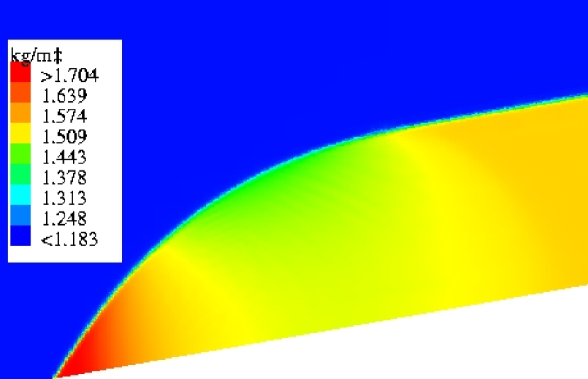
Figure 4: Left: numerical solution of the wedge flow problem. Right: Structure. Three trivial hyperbolic regions $I$, $L$, $R$ are separated by straight shocks. They enclose a nontrivial elliptic region bounded by a curved shock and two parabolic circle arcs centered in $\vec{v}_{L}$ resp. $\vec{v}_{R}$ with radius $c_{L}$ resp. $c_{R}$. Density and velocity are functions of $\xi=x/t$, $\eta=y/t$ only.

Figure 4 shows the flow pattern (density) solving our test problem, for some positive time. Here $\gamma=7/5$, $M_{I}=2.94$ and $\tau=10^{\circ}$. $\vec{v}_{I}$ is horizontal from left to right. Blue is $\rho_{I}$; green, yellow and red are successively larger densities.

A straight shock (blue to red) emanates from the wedge tip. Calculation shows that it is the weak shock. There is another straight shock on the right (blue to orange), parallel to the downstream wall. Below each straight shock lies a constant region. Both shocks are connected by a curved shock, with a nontrivial (elliptic) region below.

The flow pattern is self-similar: density and velocity are constant along rays $x=\xi t,y=\eta t$ for fixed $\xi,\eta$. This can be visualized as $t$ being a “zoom” parameter, with $t=0$ corresponding to “infinitely far away” and $t\uparrow\infty$ to “infinitely close to the origin” (wedge tip resp. wall corner). In particular the flow structure is the same for all times.

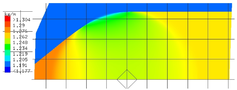
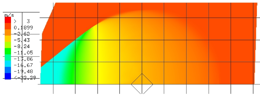
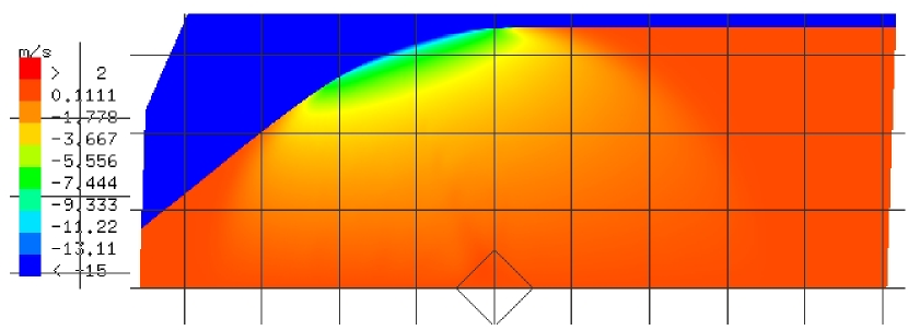
Figure 5: Elliptic region. From top to bottom: $\rho$, $\vec{v}$ tangential, and $\vec{v}$ normal to the wedge surface. Corner/wedge tip is intersection of left shock and bottom domain boundary (left outside diagrams). Diamond indicates origin in Figure 12 coordinates; velocities are relative to it.

Figure 5 shows the elliptic region in more detail. In the top picture density is shown; its minimum in the elliptic region is attained at the shock (Proposition 3.7.1 will show that the minimum is a “pseudo-normal” point). In the middle picture the velocity tangential to the downstream wall is shown; the bottom picture shows velocity normal to the downstream wall.

The diamond in the center of the bottom domain boundaries indicates the origin in self-similar coordinates, where we use standard coordinates (Figure 12).

It should be emphasized that numerical computations only suggest the structure of the solution. For instance, it is not clear that the constant states $L$ and $R$ extend to the pseudo-sonic circles $P_{L}$ and $P_{R}$. Although in one dimension with viscosity, some techniques can convert a numerical solution with sufficiently small residual into an existence proof for an exact solution (see e.g. [JY98]), only partial results are available in multiple dimensions without viscosity (see [Kuz75, LW60, Ell07]); it is not clear whether a general result is even true (see [Ell06]).

1.3 Main result

To obtain a mathematical argument, we construct the self-similar solution exactly rather than numerically. We use compressible potential flow as model:

Theorem 1.

Let $\tau\in(0,\frac{\pi}{2})$, $M_{I},\rho_{I},c_{I}\in(0,\infty)$, $\gamma\in[1,\infty)$; set $\vec{v}_{I}:=(M_{I}c_{I},0)$. Define the wedge

$$W :=\{(x,y)\in\mathds{R}^{2}:y<x\tan\tau\}$$

and

$$\Omega :=(0,\infty)\times\complement W.$$

Assume the following conditions are satisfied:

1. Unsteady potential flow with $\gamma$-law pressure admits a steady straight shock with upstream data $\rho_{I}$ and $\vec{v}_{I}$ and downstream velocity $\vec{v}_{L}$ and sound speed $c_{L}$ so that

   $$\measuredangle(\vec{v}_{I},\vec{v}_{L})=\tau.$$

2. The shock is supersonic-supersonic:

   $$M_{L}:=\frac{|\vec{v}_{L}|}{c_{L}}>1.$$

3. Of the two intersection points of the shock with the circle $\partial B_{c_{L}}(\vec{v}_{L})$, let $\vec{\xi}^{*}_{L}$ be the one closer to the corner (origin). Let the $R$ shock be the unique shock parallel to $\vec{v}_{L}$, with upstream data $\rho_{I}$ and $\vec{v}_{I}$, downstream sound speed $c_{R}$ and downstream velocity $\vec{v}_{R}$ parallel to $\vec{v}_{L}$ as well. Of the two intersection points with $\partial B_{c_{R}}(\vec{v}_{R})$, let $\vec{\xi}^{*}_{R}$ be the one farther from the corner (see Figure 6). We require that

   $$\{\text{Line segment from $\vec{\xi}^{*}_{L}$ to $\vec{\xi}^{*}_{R}$}\}\cap\overline{B}_{c_{I}}(\vec{v}_{I}) =\emptyset.$$ (1.3.1)

Then there is a weak solution (see Remark 1.3.1) $\phi\in C^{0,1}(\overline{\Omega})$ of

unsteady potential flow in $$\Omega$$, (1.3.2)

$$\nabla\phi\cdot\vec{n}=0\qquad \partial W$$ on , (1.3.3)

$$\rho=\rho_{I},\quad\nabla\phi=\vec{v}_{I}\qquad t=0$$ for (1.3.4)

Figure 6: Solutions are constructed for all cases that satisfy the condition (1.3.1): the dashed circle and line must be separated. A shock has positive strength if and only if it does not touch the circle.

In addition to existence, detailed results about the structure of the weak solution can be obtained (see Remark 4.16.2). At this point we emphasize only that each solution consists, in some neighbourhood of the origin, of the weak shock separating two constant-state regions.

Remark 1.3.1.

See Section 2.1 for introduction and precise definition of potential flow. By weak solution we mean that

$$\nabla\phi(0,\vec{x}) =\vec{v}_{I}\qquad\text{for a.e.\ $\vec{x}\in\complement W$}$$ (1.3.5)

and

$$\int_{\Omega}\rho\vartheta_{t}+\rho\nabla\phi\cdot\nabla\vartheta~{}d\vec{x}~{}dt+\int_{\complement W}\vartheta(0,x,y)\rho_{I}~{}d\vec{x} =0$$

for all test functions $\vartheta\in C_{c}^{\infty}(\overline{\Omega})$.

(For $\phi\in C^{0,1}(\overline{\Omega})$, the velocity $\nabla\phi$ is a.e. well-defined on $\{0\}\times\complement W$, but $\phi_{t}$ and hence $\rho$ may not be well-defined.)

Remark 1.3.2.

As Remark 4.16.1 shows, there is a large set of tip shocks and parameters that satisfy the conditions of Theorem 1.

The first and second condition are physically necessary, not technical limitations. If the first is violated (for $M_{I}<1$ or large $\tau$), there is no straight steady physical shock attached to the corner at all. If either of them is violated, numerical experiments show a flow pattern with a shock detached from the corner, moving upstream (left).

The third condition is technical. It is needed in some cases to prove the shock does not vanish (which is never observed in numerics); none of the other estimates requires this condition. We expect that the condition will be removed with some additional analysis.

It should be emphasized that the theorem and its proof are global in nature: large parameter changes are possible.

Remark 1.3.3.

Incidentally we also solve the problem for asymmetric wedges, as long as both sides allow a supersonic-supersonic weak shock and as long as (1.3.1) is satisfied on both sides.

1.4 Related work

[CF48, Section 117, 122 and 123] explain in detail shock polars and the corner flow problem. Despite its age, its discussion of weak vs. strong shock is still a good reflection of the state of prior research. [FT68] is another useful reference.

[ČanićKK02] consider the classical problem of regular reflection of a shock by a symmetric wedge; this problem, like ours, has a self-similar solution. They consider the unsteady transonic small disturbance equation as model. [Zhe06] studies the same problem for the pressure-gradient system. The monographs [Zhe01, LZY98] compute various self-similar flows numerically and present some analysis and simplified models.

[CF03] prove existence of small perturbations of a plane shock in steady potential flow.

[Che03] constructs steady solutions for 3D cones rather than 2D wedges. [LL99] discuss stability of 3D flow past a perturbed cone; [CL05] show existence and linear stability in the case of the isentropic Euler equations. [CZZ06] study existence and stability of supersonic flows onto perturbed wedges with attached shocks; the introduction gives a detailed discussion of previous work.

So far the only other paper that proves global existence of some nontrivial time-dependent solution of potential flow is [CF]: they construct exact solutions for regular reflection, assuming sufficiently sharp wedges.

1.5 Overview

In Section 2 we give an introduction to unsteady potential flow. We derive self-similar potential flow, discuss its shock conditions and analyze the properties of shocks in detail.

In Section 3 we discuss a collection of maximum principles for elliptic regions of self-similar potential flow. Some of these identify circumstances in which certain quantities (density, …) can or cannot have maxima or minima in the interior. Other results discuss local extrema at solid (slip condition) walls and finally shocks with a constant-state hyperbolic region on the other side.

Since the hyperbolic regions are trivial (see Figure 4), the heart of the problem is the construction of the elliptic region. This is accomplished in Section 4. Readers interested in more overview should go to Section 4.2, where all proof steps are surveyed.

A crucial ingredient are the maximum principles from Section 3, combined with ODE-type arguments at the parabolic arcs in Sections 4.6 to 4.10, and techniques to control shock location and normals (Sections 4.11 and 4.12). Section 4.16 combines the elliptic region with its hyperbolic counterparts to construct the full flow pattern. The remaining sections are standard but delicate applications of nonlinear elliptic theory. Some literature results, such as regularity in corners and at free boundaries, need extension which is done in the Appendix.

1.6 Notation

For the most part we use standard notation. Subscripts and superscripts may denote tensor indices, partial derivatives or powers, depending on the context.

$\measuredangle(\vec{x},\vec{y})$ is the counterclockwise angle from $\vec{x}$ to $\vec{y}$. For $\vec{x}=(x_{1},x_{2})$, $\vec{y}=(y_{1},y_{2})$,

$$\vec{x}^{\perp}:=(-x_{2},x_{1})$$

(counterclockwise rotation by $90^{\circ}$),

$$\vec{x}\times\vec{y}:=x_{1}y_{2}-x_{2}y_{1}.$$

$\vec{x}^{2}$ is the rank-one matrix $\vec{x}\vec{x}^{T}$ whereas $|\vec{x}|^{2}$ is the norm. Correspondingly, $\nabla^{2}=\nabla\nabla^{T}$ is the Hessian (not the Laplacian).

Normals $\vec{n}$ are outer normals to a domain, except on the shock $S$ (defined later) where they are downstream, so usually inner. Tangents $\vec{t}$ are always defined as $\vec{t}:=\vec{n}^{\perp}$.

2 Potential flow

2.1 Unsteady potential flow

We consider the isentropic Euler equations of compressible gas dynamics in $d$ space dimensions:

$$\rho_{t}+\nabla\cdot(\rho\vec{v}) =0$$ (2.1.1)

$$(\rho\vec{v})_{t}+\sum_{i=1}^{d}(\rho v^{i}\vec{v})_{x^{i}}+\nabla(p(\rho)) =0,$$ (2.1.2)

Hereafter, $\nabla$ denotes the gradient with respect either to the space coordinates ${\vec{x}}=(x^{1},x^{2},\cdots,x^{d})$ or the similarity coordinates $t^{-1}\vec{x}$. ${\vec{v}}=(v^{1},v^{2},\cdots,v^{d})$ is the velocity of the gas, $\rho$ the density, $p(\rho)$ pressure. In this article we consider only polytropic pressure laws ($\gamma$-laws) with $\gamma\geq 1$:

$$p(\rho) =\frac{c_{0}^{2}\rho_{0}}{\gamma}\left(\frac{\rho}{\rho_{0}}\right)^{\gamma}$$ (2.1.3)

(here $c_{0}$ is the sound speed at density $\rho_{0}$). Many subsequent results extend with little or no change to $\gamma<1$ or to general pressure laws, but in special cases some steps require more work or break down entirely. To keep the presentation simple we don’t strive for generality with respect to pressure laws.

For smooth solutions, substituting (2.1.1) into (2.1.2) yields the simpler form

$$\vec{v}_{t}+\vec{v}\cdot\nabla^{T}\vec{v}+\nabla(\pi(\rho)) =0.$$ (2.1.4)

Here $\pi$ is defined as

$$\pi(\rho) =c_{0}^{2}\cdot\begin{cases}\frac{(\rho/\rho_{0})^{\gamma-1}-1}{\gamma-1},&\gamma>1\\ \log(\rho/\rho_{0}),&\gamma=1.\end{cases}$$

This $\pi$ is $C^{\infty}$ in $\rho\in(0,\infty)$ and $\gamma\in[1,\infty)$ and has the property

$$\pi_{\rho}=\frac{p_{\rho}}{\rho}.$$

If we assume irrotationality

$$v^{i}_{j}=v^{j}_{i}$$

(where $i,j=1,\dotsc,d$), then the Euler equations are reduced to potential flow:

$$\vec{v} =\nabla_{\vec{x}}\phi$$

for some scalar potential function $\phi$. For smooth flows, substituting this into (2.1.4) yields, for $i=1,\dotsc,d$,

$$0 =\phi_{it}+\nabla\phi_{i}\cdot\nabla\phi+\pi(\rho)_{i}=\big{(}\phi_{t}+\frac{|\nabla\phi|^{2}}{2}+\pi(\rho)\big{)}_{i}.$$

Thus, for some constant $A$,

$$\rho =\pi^{-1}(A-\phi_{t}-\frac{|\nabla\phi|^{2}}{2}).$$ (2.1.5)

Substituting this into (2.1.1) yields a single second-order quasilinear hyperbolic equation, the potential flow equation, for a scalar field $\phi$:

$$\big{(}\rho(\phi_{t},|\nabla\phi|)\big{)}_{t}+\nabla\cdot\big{(}\rho(\phi_{t},|\nabla\phi|)\nabla\phi\big{)} =0.$$ (2.1.6)

Henceforth we omit the arguments of $\rho$. Moreover we eliminate $A$ with the substitution

$$A\leftarrow 0,\qquad\phi(t,\vec{x})\leftarrow\phi(t,\vec{x})-tA$$

(so that $\phi_{t}\leftarrow\phi_{t}-A$). Hence we use

$$\rho =\pi^{-1}(-\phi_{t}-\frac{1}{2}|\nabla\phi|^{2})$$ (2.1.7)

from now on.

Using $c^{2}=p_{\rho}$ and

$$(\pi^{-1})^{\prime} =(\pi_{\rho})^{-1}=(\frac{p_{\rho}}{\rho})^{-1}=\frac{\rho}{c^{2}}$$ (2.1.8)

the equation can also be written in nondivergence form:

$$\phi_{tt}+2\nabla\phi_{t}\cdot\nabla\phi+\sum_{i,j=1}^{d}\phi_{i}\phi_{j}\phi_{ij}-c^{2}\Delta\phi =0$$ (2.1.9)

(2.1.9) is hyperbolic (as long as $c>0$). For polytropic pressure law the local sound speed $c$ is given by

$$c^{2} =c_{0}^{2}+(\gamma-1)(-\phi_{t}-\frac{1}{2}|\nabla\phi|^{2}).$$ (2.1.10)

2.2 Self-similar potential flow

Our initial data is self-similar: it is constant along rays emanating from $\vec{x}=(0,0)$. Our domain $\complement W$ is self-similar too: it is a union of rays emanating from $(t,x,y)=(0,0,0)$. In any such situation it is expected — and confirmed by numerical results — that the solution is self-similar as well, i.e. that $\rho,\vec{v}$ are constant along rays $\vec{x}=t\vec{\xi}$ emanating from the origin. Self-similarity corresponds to the ansatz

$$\phi(t,\vec{x}) :=t\psi(\vec{\xi}),\qquad\vec{\xi}:=t^{-1}\vec{x}.$$ (2.2.1)

Clearly, $\phi\in C^{0,1}(\Omega)$ if and only if $\psi\in C^{0,1}(\complement W)$. This choice yields

$$\vec{v}(t,\vec{x}) =\nabla\phi(t,\vec{x})=\nabla\psi(t^{-1}\vec{x}),$$

$$\rho(t,\vec{x}) =\pi^{-1}(-\phi_{t}-\frac{1}{2}|\nabla\phi|^{2})=\pi^{-1}(-\psi+\vec{\xi}\cdot\nabla\psi-\frac{1}{2}|\nabla\psi|^{2}).$$

The expression for $\rho$ can be made more pleasant (and independent of $\vec{\xi}$) by using

$$\chi(\vec{\xi}) :=\psi(\vec{\xi})-\frac{1}{2}|\vec{\xi}|^{2};$$

this yields

$$\rho =\pi^{-1}(-\chi-\frac{1}{2}|\nabla\chi|^{2}).$$ (2.2.2)

$\nabla\chi=\nabla\psi-\vec{\xi}$ is called pseudo-velocity.

(2.1.6) then reduces to

$$\nabla\cdot(\rho\nabla\chi)+2\rho =0$$ (2.2.3)

(or $+d\rho$, in $d$ dimensions) which holds in a distributional sense. For smooth solutions we obtain the non-divergence form

$$(c^{2}I-\nabla\chi\nabla\chi^{T}):\nabla^{2}\chi=(c^{2}-\chi_{\xi}^{2})\chi_{\xi\xi}-2\chi_{\xi}\chi_{\eta}\chi_{\xi\eta}+(c^{2}-\chi_{\eta}^{2})\chi_{\eta\eta} =|\nabla\chi|^{2}-2c^{2}$$ (2.2.4)

Another convenient form is

$$(c^{2}I-\nabla\chi\nabla\chi^{T}):\nabla^{2}\psi =(c^{2}-\chi_{\xi}^{2})\psi_{\xi\xi}-2\chi_{\xi}\chi_{\eta}\psi_{\xi\eta}+(c^{2}-\chi_{\eta}^{2})\psi_{\eta\eta}=0.$$ (2.2.5)

Here, (2.1.10) for polytropic pressure law yields

$$c^{2} =c_{0}^{2}+(\gamma-1)(-\chi-\frac{1}{2}|\nabla\chi|^{2})$$ (2.2.6)

Remark 2.2.1.

(2.2.3) inherits a number of symmetries from (2.1.1), (2.1.2):

1. It is invariant under rotation.

2. It is invariant under reflection.

3. It is invariant under translation in $\vec{\xi}$, which is not as trivial as translation in $\vec{x}$: it corresponds to the Galilean transformation $\vec{v}\leftarrow\vec{v}+\vec{v}_{0}$, $\vec{x}\leftarrow\vec{x}-\vec{v}_{0}t$ (with constant $\vec{v}_{0}\in\mathds{R}^{d}$) in $(t,\vec{x})$ coordinates. This is sometimes called change of inertial frame.

(2.2.4) is a PDE of mixed type. The type is determined by the (local) pseudo-Mach number

$$L :=\frac{|\nabla\chi|}{c},$$ (2.2.7)

with $0\leq L<1$ for elliptic (pseudo-subsonic), $L=1$ for parabolic (pseudo-sonic), $L>1$ for hyperbolic (pseudo-supersonic) regions.

The pseudo-Mach number $L$ can be interpreted in a way analogous to the Mach number $M$: consider a steady solution of the unsteady potential flow equation. Loosely speaking, in an $M<1$ (subsonic) region a small localized disturbance will be propagated in all directions, whereas in an $M>1$ region it is propagated only in the Mach cone. $L<1$ and $L>1$ are analogous, except that we study the propagation of disturbances in the unsteady potential flow equation written in $(t,\vec{x}/t)$ coordinates, rather than $(t,\vec{x})$.

There is no strong relation between $M<1$ and $L<1$: consider two constant-state (hence steady and selfsimilar) flows with zero velocity ($M=0$ constant) resp. supersonic velocity $\vec{v}$ ($M>1$ constant). Each flow has $L=0$ in the point $\vec{\xi}=0$ resp. $\vec{\xi}=\vec{v}$ and $L\uparrow\infty$ as $\vec{\xi}\uparrow\infty$, so there are examples for each of the four cases $M,L<1$, $M<1<L$, $L<1<M$ and $1<L,M$.

While velocity $\vec{v}$ is motion relative to space coordinates $\vec{x}$, pseudo-velocity

$$\vec{z}:=\nabla\chi$$

is motion relative to similarity coordinates $\vec{\xi}$ at time $t=1$.

The simplest class of solutions of (2.2.4) are the constant-state solutions: $\psi$ affine in $\vec{\xi}$, hence $\vec{v}$, $\rho$ and $c$ constant. They are elliptic in a circle centered in $\vec{\xi}=\vec{v}$ with radius $c$, parabolic on the boundary of that circle and hyperbolic outside.

Convention 2.2.2.

If we study a function called (e.g.) $\tilde{\chi}$, then $\tilde{\psi}$, $\tilde{\rho}$, $\tilde{L}$ etc. will refer to the quantities computed from it as $\psi$, $\rho$, $L$ are computed from $\chi$ (e.g. $\tilde{\psi}=\tilde{\chi}+\frac{1}{2}|\vec{\xi}|^{2}$). We will tacitly use this notation from now on.

2.3 Shock conditions

Consider a ball $U$ and a simple smooth curve $S$ so that $U=U^{u}\cup S\cup U^{d}$ where $U^{u},U^{d}$ are open, connected, and $S,U^{u},U^{d}$ disjoint. Consider $\chi:U\rightarrow\mathds{R}$ so that $\chi=\chi^{u,d}$ in $U^{u,d}$ where $\chi^{u,d}\in\mathcal{C}^{2}(\overline{U^{u,d}})$.

$\chi$ is a weak solution of (2.2.3) if and only if it is a strong solution in each point of $U_{-}$ and $U_{+}$ and if it satisfies the following conditions in each point of $S$:

$$\chi^{u} =\chi^{d},$$ (2.3.1)

$$\vec{n}\cdot(\rho^{u}\nabla\chi^{u}-\rho^{d}\nabla\chi^{d}) =0$$ (2.3.2)

Here $\vec{n}$ is a normal to $S$.

(2.3.1) and (2.3.2) are the Rankine-Hugoniot conditions for self-similar potential flow shocks. They do not depend on $\vec{\xi}$ or on the shock speed explicitly; these quantities are hidden by the use of $\chi$ rather than $\psi$. The Rankine-Hugoniot conditions are derived in the same way as those for the full Euler equations (see [Eva98, Section 3.4.1]).

Note that (2.3.1) is equivalent to

$$\psi^{u} =\psi^{d}.$$ (2.3.3)

Taking the tangential derivative of (2.3.1) resp. (2.3.3) yields

$$\frac{\partial\chi^{u}}{\partial t} =\frac{\partial\chi^{d}}{\partial t},$$ (2.3.4)

$$\frac{\partial\psi^{u}}{\partial t} =\frac{\partial\psi^{d}}{\partial t}.$$ (2.3.5)

The shock relations imply that the tangential velocity is continuous across shocks.

Define $(z^{x}_{u},z^{y}_{u}):=\vec{z}_{u}:=\nabla\chi^{u}$ and $(v^{x}_{u},v^{y}_{u}):=\vec{v}_{u}:=\nabla\psi^{u}$. Abbreviate $z^{t}_{u}:=\vec{z}_{u}\cdot\vec{t}$, $z^{n}_{u}:=\vec{z}_{u}\cdot\vec{n}$, and same for $v$ instead of $z$. Same definitions for $d$ instead of $u$. We can restate the shock relations as

$$\rho_{u}z^{n}_{u} =\rho_{d}z^{n}_{d},$$ (2.3.6)

$$z_{u}^{t} =z_{d}^{t}.$$ (2.3.7)

Using the last relation, we often write $z^{t}$ without distinction.

The shock speed is $\sigma=\vec{\xi}\cdot\vec{n}$, where $\vec{\xi}$ is any point on the shock. A shock is steady in a point if its tangent passes through the origin. We can restate (2.3.6) as

$$\rho_{u}v^{n}_{u}-\rho_{d}v^{n}_{d} =\sigma(\rho_{u}-\rho_{d})$$

which is a more familiar form.

We focus on $\rho_{u},\rho_{d}>0$ from now on, which will be the case in all circumstances. If $\rho_{u}=\rho_{d}$ in a point, we say the shock vanishes; in this case $z^{n}_{d}=z^{n}_{u}$ in that point, by (2.3.7). In all other cases $z^{n}_{d},z^{n}_{u}$ must have equal sign by (2.3.7); we fix $\vec{n}$ so that $z^{n}_{d},z^{n}_{u}>0$. This means the normal points downstream. The shock is admissible if and only if $\rho_{u}\leq\rho_{d}$ which is equivalent to $z^{n}_{u}\geq z^{n}_{d}$.

A shock is called pseudo-normal in a point $\vec{\xi}$ if $z^{t}=0$ there. For $\vec{\xi}=0$, this means that the shock is normal ($v^{t}=0$), but for $\vec{\xi}\neq 0$ normal and pseudo-normal are not always equivalent.

It is good to keep in mind that for a straight shock, $\rho_{d}$ and $\vec{v}_{d}$ are constant if $\rho_{u}$ and $\vec{v}_{u}$ are. Obviously $\vec{z}_{d}$ may vary in this case.

Remark 2.3.1.

The Rankine-Hugoniot conditions for the original isentropic Euler equations cannot be used for potential flow: even if the flow on one side of a shock is irrotational, the flow on the other side has nonzero vorticity for curved shocks.

2.4 Pseudo-normal shocks

Here we study the consequences and solutions of the shock relations in a pseudo-normal point. We state all results for pseudo-velocities $\vec{z}$ and for pseudo-Mach numbers $L$ because moving shocks are ubiquitous in this article. For better intuition the reader may bear in mind that $\vec{z}=\vec{v}$ and $L=M$ if the shock is steady, i.e. passes through the origin. In fact by Remark 2.2.1, weak and entropy solutions of self-similar potential flow are invariant under translation and rotation, so we may always consider translating the shock so that it becomes steady, which does not change $\vec{z},\rho,L$ whereas $\vec{v}$ is changed only by a constant vector. Hence the behaviour of arbitrary shocks is entirely determined by those of steady shocks.

$L^{n}:=z^{n}/c$ and $L^{t}:=z^{t}/c$ will be referred to as normal resp. tangential pseudo-Mach number. (2.3.1) and (2.2.2) imply

$$\rho_{d} =\pi^{-1}(\pi(\rho_{u})+\frac{|z_{u}|^{2}}{2}-\frac{|z_{d}|^{2}}{2}).$$ (2.4.1)

It is apparent that (2.4.1) reduces to

$$\rho_{d} =\pi^{-1}(\pi(\rho_{u})+\frac{(z^{n}_{u})^{2}}{2}-\frac{(z^{n}_{d})^{2}}{2}).$$ (2.4.2)

Combined with (2.3.7) there is a direct relation between normal velocities, independent of the tangential velocities.

For polytropic pressure laws we may use a rather convenient simplification: there is an explicit relation connecting $L^{n}_{u},L^{n}_{d}$, independent of $\rho_{u},\vec{z}_{u}$.

Lemma 2.4.1.

For $L^{n}_{u},L^{n}_{d}>0$, (2.4.2) and (2.3.6) are equivalent to

$$g(L^{n}_{u}) =g(L^{n}_{d}),$$ (2.4.3)

$$g(x) =\begin{cases}\left(x^{2}+\frac{2}{\gamma-1}\right)x^{\frac{2(1-\gamma)}{\gamma+1}},&\gamma>1,\\ x^{2}-2\log x,&\gamma=1.\end{cases}$$ (2.4.4)

Note that

$$\frac{\partial g}{\partial x} =\frac{4}{\gamma+1}(x-x^{-1})x^{-2\frac{\gamma-1}{\gamma+1}},$$ (2.4.5)

$$\frac{\partial^{2}g}{\partial x^{2}} =\frac{4}{(\gamma+1)^{2}}\big{(}(3-\gamma)+(3\gamma-1)x^{-2}\big{)}x^{-2\frac{\gamma-1}{\gamma+1}}.$$ (2.4.6)

$$g(x) \sim\begin{cases}x^{-2\frac{\gamma-1}{\gamma+1}},&\gamma>1\\ -\log x,&\gamma=1\end{cases}\qquad\text{as $x\downarrow 0$,}$$ (2.4.7)

$$g(x) \sim x^{\frac{4}{\gamma+1}}\qquad\text{as $x\uparrow\infty$,}$$ (2.4.8)

Moreover

$$\frac{c_{u}}{c_{d}} =\left(\frac{L^{n}_{d}}{L^{n}_{u}}\right)^{\frac{\gamma-1}{\gamma+1}}.$$ (2.4.9)

as well as

$$\frac{\rho_{u}}{\rho_{d}} =\left(\frac{L^{n}_{d}}{L^{n}_{u}}\right)^{\frac{2}{\gamma+1}}.$$ (2.4.10)

Proof.

(2.3.6) can be written

$$\rho_{u}L^{n}_{u}c_{u} =\rho_{d}L^{n}_{d}c_{d}$$

$$\Rightarrow\qquad(\rho_{u})^{(\gamma+1)/2}L^{n}_{u} =\rho_{d}^{(\gamma+1)/2}L^{n}_{d};$$ (2.4.11)

this yields (2.4.10) which yields (2.4.9).

Consider $\gamma>1$, so that $c^{2}=c_{0}^{2}+(\gamma-1)\pi(\rho)$. (2.4.2) can be transformed to

$$\frac{(z^{n}_{u})^{2}}{2}+\frac{c_{u}^{2}}{\gamma-1} =\frac{(z^{n}_{d})^{2}}{2}+\frac{c_{d}^{2}}{\gamma-1}$$

$$\Leftrightarrow\quad\left((L^{n}_{u})^{2}+\frac{2}{\gamma-1}\right)c_{u}^{2} =\left((L^{n}_{d})^{2}+\frac{2}{\gamma-1}\right)c_{d}^{2}$$

Substitute (2.4.9) to obtain (2.4.3).

For $\gamma=1$, (2.4.2) is

$$c_{0}^{2}\log\frac{\rho_{d}}{\rho_{0}}+\frac{(z^{n}_{d})^{2}}{2} =c_{0}^{2}\log\frac{\rho_{u}}{\rho_{0}}+\frac{(z^{n}_{u})^{2}}{2}$$

$$\Rightarrow\qquad\frac{\rho_{d}}{\rho_{u}} =\exp\frac{(L^{n}_{u})^{2}-(L^{n}_{d})^{2}}{2};$$

using (2.4.10) we obtain (2.4.3). ∎

Proposition 2.4.2.

There is an analytic strictly decreasing function $L^{n}_{d}=L^{n}_{d}(L^{n}_{u})$, which is its own inverse, so that the shock relation (2.4.3) is solved for all $L^{n}_{u}\in(0,\infty)$. For $L^{n}_{u}\neq 1$, the only other solution of (2.4.3) is the trivial one: $L^{n}_{d}=L^{n}_{u}$. For $L^{n}_{u}=1$, both coincide.

$$L^{n}_{d} \begin{cases}\uparrow\infty,&L^{n}_{u}\downarrow 0,\\ =1,&L^{n}_{u}=1,\\ \sim(L^{n}_{u})^{\frac{-2}{\gamma-1}},&L^{n}_{u}\uparrow\infty,\ \gamma>1,\\ \sim\exp(-\frac{(L^{n}_{u})^{2}}{2}),&L^{n}_{u}\uparrow\infty,\ \gamma=1.\end{cases}$$ (2.4.12)

The resulting shock is admissible if and only if $L^{n}_{u}\geq 1$.

$$\frac{\partial L^{n}_{d}}{\partial L^{n}_{u}} =\frac{L^{n}_{u}-1/L^{n}_{u}}{L^{n}_{d}-1/L^{n}_{d}}\left(\frac{L^{n}_{u}}{L^{n}_{d}}\right)^{-2\frac{\gamma-1}{\gamma+1}}<0,$$ (2.4.13)

$$\frac{\partial L^{n}_{d}}{\partial L^{n}_{u}}_{|L^{n}_{u}=L^{n}_{d}(=1)} =-1,$$ (2.4.14)

For $L^{n}_{u}>1>L^{n}_{d}$, we have $\rho_{d}>\rho_{u}$ and $z^{n}_{d}<z^{n}_{u}$. $\rho_{d},c_{d}$ are strictly increasing in $L^{n}_{u}$ for $\rho_{u}$ fixed. For $\gamma>1$, $c_{d}>c_{u}$ as well, and $c_{d}$ is strictly increasing in $L^{n}_{u}$ for $\rho_{u}$ fixed.

Proof.

Assume $L^{n}_{u}>1$. From (2.4.5) it is obvious that $\frac{\partial g}{\partial x}(x)>0$ for $x>1$. Hence $g(L^{n}_{u})>g(1)$; moreover (2.4.3) cannot have more than one solution $L^{n}_{d}$ in $[1,\infty]$ for fixed $L^{n}_{u}\geq 1$; in fact $L^{n}_{d}=L^{n}_{u}$ is the unique solution. For $x<1$, $\frac{\partial g}{\partial x}(x)<0$, so (2.4.3) cannot have more than one solution $L^{n}_{d}$ in $(0,1)$. It must have one, though, because $g(0+)=+\infty>g(L^{n}_{u})>g(1)$.

For $L^{n}_{u}<1$, the existence of a nontrivial solution $L^{n}_{d}\in(1,\infty)$ is obtained from the previous case by analogous arguments. For $L^{n}_{u}=1$, the sign of $\partial g/\partial x$ rules out any other solutions. Since (2.4.3) is symmetric in $L^{n}_{u},L^{n}_{d}$, it is obvious that $L^{n}_{u}\mapsto L^{n}_{d}$ is its own inverse.

The trivial solution branch $L^{n}_{d}=L^{n}_{u}$ is obviously smooth; by the implicit function theorem the the nontrivial branch is analytic away from $L^{n}_{u}=1$. In $L^{n}_{u}=1$ there is a degeneracy which has to be analyzed by inspecting the Hessian of $h(L^{n}_{u},L^{n}_{d}):=g(L^{n}_{u})-g(L^{n}_{d})=0$:

$$A:=\begin{bmatrix}\frac{\partial^{2}h}{(\partial L^{n}_{u})^{2}}&\frac{\partial^{2}h}{\partial L^{n}_{u}\partial L^{n}_{d}}\\ \frac{\partial^{2}h}{\partial L^{n}_{u}\partial L^{n}_{d}}&\frac{\partial^{2}h}{(\partial L^{n}_{d})^{2}}\end{bmatrix} =\begin{bmatrix}\frac{\partial^{2}g}{\partial x^{2}}(L^{n}_{u})&0\\ 0&\frac{-\partial^{2}g}{\partial x^{2}}(L^{n}_{d})\end{bmatrix}_{|L^{n}_{u}=L^{n}_{d}=1}\overset{\text{(\ref{eq:ddgddM})}}{=}\begin{bmatrix}\frac{8}{\gamma+1}&0\\ 0&\frac{-8}{\gamma+1}\end{bmatrix}.$$

$A$ is an invertible indefinite matrix; the solutions of $\vec{w}^{T}A\vec{w}=0$ are $\vec{w}=(1,1)$ and $\vec{w}=(1,-1)$. The classical Morse lemma (see e.g. [Smo94, Lemma 12.19]) shows that in a small neighbourhood of $(L^{n}_{u},L^{n}_{d})=(1,1)$, the solution of (2.4.3) form two analytic curves that intersect in $(1,1)$ with tangents $(1,1)$ (trivial branch) and $(1,-1)$ (nontrivial branch). The latter yields (2.4.14).

The remainder of (2.4.12) follows from the asymptotics of $g$ (see (2.4.7), (2.4.8)).

From (2.4.10) and (2.4.13) we see that $\rho_{d}>\rho_{u}$ for $L^{n}_{d}<1<L^{n}_{u}$ and that $\rho_{d}$ is an increasing function of $L^{n}_{u}$ for $\rho_{u}$ held fixed. Clearly the same applies to $c_{d}$ if $\gamma>1$, and (because of (2.3.6)) $z^{n}_{d}<z^{n}_{u}$. This means the shock is admissible for $L^{n}_{u}>1$. ∎

Remark 2.4.3.

In the remaining arguments we always assume that the shock is admissible (or vanishing) and ignore the branch $L^{n}_{d}=L^{n}_{u}$.

Proposition 2.4.4.

If we hold $c_{u},\rho_{u}$ fixed:

$$\frac{z^{n}_{u}}{z^{n}_{d}}\cdot\frac{\partial z^{n}_{d}}{\partial z^{n}_{u}}<\frac{\gamma-1}{\gamma+1}<1.$$ (2.4.16)

In particular

$$\frac{\partial z^{n}_{d}}{\partial z^{n}_{u}}<\frac{\gamma-1}{\gamma+1}.$$ (2.4.17)

Therefore

$$\frac{z^{n}_{d}}{c_{u}}-1<\frac{\gamma-1}{\gamma+1}\Big{(}\frac{z^{n}_{u}}{c_{u}}-1\Big{)}$$ (2.4.18)

Remark 2.4.5.

(2.4.17) is not very tight (we can show $<0$ for $\gamma<3$), but sufficient for our purposes.

Proof.

We use (2.4.9):

$$\frac{\partial c_{d}}{\partial L^{n}_{u}} =c_{u}\frac{\partial}{\partial L^{n}_{u}}\left(\frac{L^{n}_{u}}{L^{n}_{d}}\right)^{\frac{\gamma-1}{\gamma+1}}=\frac{c_{u}}{L^{n}_{d}}\left(\frac{L^{n}_{u}}{L^{n}_{d}}\right)^{\frac{-2}{\gamma+1}}\frac{\gamma-1}{\gamma+1}\left(1-\frac{L^{n}_{u}}{L^{n}_{d}}\frac{\partial L^{n}_{d}}{\partial L^{n}_{u}}\right)$$

so

$$\frac{\partial z^{n}_{d}}{\partial z^{n}_{u}} =c_{u}^{-1}\frac{\partial z^{n}_{d}}{\partial L^{n}_{u}}=\frac{L^{n}_{d}}{c_{u}}\frac{\partial c_{d}}{\partial L^{n}_{u}}+\frac{c_{d}}{c_{u}}\frac{\partial L^{n}_{d}}{\partial L^{n}_{u}}$$

$$\overset{(\ref{eq:cM})}{=}\left(\frac{L^{n}_{u}}{L^{n}_{d}}\right)^{\frac{-2}{\gamma+1}}\left(\frac{2}{\gamma+1}\cdot\frac{L^{n}_{u}}{L^{n}_{d}}\cdot\frac{\partial L^{n}_{d}}{\partial L^{n}_{u}}+\frac{\gamma-1}{\gamma+1}\right)$$

Then

$$\frac{z^{n}_{u}}{z^{n}_{d}}\frac{\partial z^{n}_{d}}{\partial z^{n}_{u}} =\frac{\rho_{d}}{\rho_{u}}\left(\frac{L^{n}_{u}}{L^{n}_{d}}\right)^{\frac{-2}{\gamma+1}}\left(\frac{2}{\gamma+1}\cdot\frac{L^{n}_{u}}{L^{n}_{d}}\cdot\frac{\partial L^{n}_{d}}{\partial L^{n}_{u}}+\frac{\gamma-1}{\gamma+1}\right)$$

$$\overset{(\ref{eq:rhoM})}{=}\mathord{\underbrace{\mathop{\frac{2}{\gamma+1}}}_{>0}}\cdot\mathord{\underbrace{\mathop{\frac{L^{n}_{u}}{L^{n}_{d}}}}_{>0}}\cdot\mathord{\underbrace{\mathop{\frac{\partial L^{n}_{d}}{\partial L^{n}_{u}}}}_{<0}}+\frac{\gamma-1}{\gamma+1}<\frac{\gamma-1}{\gamma+1}.$$

Integrating (2.4.17) from $z^{n}_{d}=z^{n}_{u}=c_{u}$ for a vanishing shock, we obtain (2.4.18). ∎

Proposition 2.4.6.

Consider a shock with velocity $\sigma:=\vec{\xi}\cdot\vec{n}$. Our convention $z^{n}_{u}>0$ requires $\sigma<v^{n}_{u}$. Vary $\sigma$ while holding $\vec{n}$ and $\vec{v}_{u}$ fixed. Then:

$$\frac{\partial v^{n}_{d}}{\partial\sigma} \geq 1-\frac{\partial z^{n}_{d}}{\partial z^{n}_{u}}>0;$$ (2.4.19)

$$\qquad\frac{\partial\rho_{d}}{\partial\sigma} <0.$$ (2.4.20)

Proof.

For moving shocks, $v^{n}_{d}=z^{n}_{d}+\sigma$ and $z^{n}_{u}=v^{n}_{u}-\sigma$, so

$$\frac{\partial v^{n}_{d}}{\partial\sigma} =1+\frac{\partial z^{n}_{d}}{\partial\sigma}=1-\frac{\partial z^{n}_{d}}{\partial z^{n}_{u}}\overset{\text{(\ref{eq:DvndDvnu})}}{>}1-\frac{\gamma-1}{\gamma+1}=\frac{2}{\gamma+1}>0$$

and

$$\frac{\partial\rho_{d}}{\partial\sigma} =-\frac{\partial\rho_{d}}{\partial z^{n}_{u}}=-\frac{\partial\rho_{d}}{\partial L^{n}_{u}}c_{u}^{-1}\overset{\text{(\ref{eq:rhoM})}}{\underset{\text{(\ref{eq:dMRdMLgen})}}{<}}0$$

∎

2.5 Shock polar

Here we prove only the results needed for our purposes.

Proposition 2.5.1.

Consider a fixed point on a shock with upstream density $\rho_{u}$ and pseudo-velocity $\vec{z}_{u}$ held fixed while we vary the normal. Define $\beta:=\measuredangle(\vec{z}_{u},\vec{n})$. $\rho_{d}$ is strictly decreasing in $|\beta|$, whereas $L_{d},|\vec{z}_{d}|$ are strictly increasing. $c_{d}$ is strictly decreasing for $\gamma>1$, constant otherwise. Moreover

$$(\partial_{\beta}\vec{v}_{d})\cdot\vec{n}=(\partial_{\beta}\vec{z}_{d})\cdot\vec{n} =z^{t}\Big{(}\frac{\partial z^{n}_{d}}{\partial z^{n}_{u}}-1\Big{)},$$ (2.5.1)

$$(\partial_{\beta}\vec{v}_{d})\cdot\vec{t}=(\partial_{\beta}\vec{z}_{d})\cdot\vec{t} =z^{n}_{d}-z^{n}_{u}.$$ (2.5.2)

If $\vec{z}_{u}=(z^{x}_{u},0)$ with $z^{x}_{u}>0$, then $z^{x}_{d}$ is increasing in $|\beta|$.

Proof.

$$\partial_{\beta}\vec{z}_{d} =\partial_{\beta}(z^{n}_{d}\vec{n}+z^{t}\vec{t})=\frac{\partial z^{n}_{d}}{\partial z^{n}_{u}}\partial_{\beta}z^{n}_{u}\vec{n}+z^{n}_{d}\vec{t}-z^{t}\vec{n}+\partial_{\beta}z^{t}\vec{t}$$

$$=z^{t}\Big{(}\frac{\partial z^{n}_{d}}{\partial z^{n}_{u}}-1\Big{)}\vec{n}+(z^{n}_{d}-z^{n}_{u})\vec{t}$$ (2.5.3)

This is (2.5.1), (2.5.2), using that $\vec{\xi}$ is fixed. For $\beta>0$, $z^{t}=-|\vec{z}_{u}|\sin\beta$ is strictly decreasing (and negative).

$$\frac{1}{2}\partial_{\beta}(|\vec{z}_{d}|^{2}) =\frac{1}{2}\partial_{\beta}((z^{n}_{d})^{2}+(z^{t})^{2})=z^{n}_{d}\frac{\partial z^{n}_{d}}{\partial z^{n}_{u}}\partial_{\beta}z^{n}_{u}+z^{t}\partial_{\beta}z^{t}$$

$$=z^{t}\Big{(}z^{n}_{d}\frac{\partial z^{n}_{d}}{\partial z^{n}_{u}}-\mathord{\underbrace{\mathop{z^{n}_{u}}}_{\geq z^{n}_{d}}}\Big{)}\geq\mathord{\underbrace{\mathop{z^{t}}}_{<0}}\mathord{\underbrace{\mathop{z^{n}_{d}}}_{>0}}\Big{(}\mathord{\underbrace{\mathop{\frac{\partial z^{n}_{d}}{\partial z^{n}_{u}}}}_{\leq(\gamma-1)/(\gamma+1)}}-1\Big{)}>0$$

by (2.4.17), so $|\vec{z}_{d}|$ is strictly increasing. Then by (2.4.1)

$$\rho_{d}=\pi^{-1}\big{(}\pi(\rho_{u})+\frac{1}{2}(|\vec{z}_{u}|^{2}-|\vec{z}_{d}|^{2})\big{)},$$

is strictly decreasing, as is $c_{d}$ (except constant for $\gamma=1$), so $L_{d}=|\vec{z}_{d}|/c_{d}$ is increasing.

For $\beta>0$, (2.5.3) yields

$$\partial_{\beta}(z^{x}_{d}) =\mathord{\underbrace{\mathop{z^{t}}}_{<0}}\mathord{\underbrace{\mathop{\Big{(}\frac{\partial z^{n}_{d}}{\partial z^{n}_{u}}-1\Big{)}}}_{<0}}\mathord{\underbrace{\mathop{\cos\beta}}_{>0}}-\mathord{\underbrace{\mathop{(z^{n}_{d}-z^{n}_{u})}}_{<0}}\mathord{\underbrace{\mathop{\sin\beta}}_{>0}}>0$$

by (2.4.17).

$\beta<0$ is analogous by symmetry. ∎

2.6 Shock-parabolic corners with fixed vertical downstream velocity

The corners of our elliptic region (see Figure 12) are points on shocks where $L_{d}=1$ (or $L_{d}=\sqrt{1-\epsilon}$ if regularized); on the other hand $v^{y}_{d}=0$ (if the $x$ direction is tangential to the wall). We study such shocks in detail.

Proposition 2.6.1.

Consider a straight shock (see Figure 7) passing through a point $\vec{\xi}$. The shock is pseudo-normal in the point $\vec{\xi}_{M}=\vec{\xi}+\vec{t}\cdot(\vec{v}_{d}-\vec{\xi})\vec{t}$ and pseudo-oblique in every other point. $\vec{\xi}_{M}$ is the closest point on the shock both to $\vec{v}_{u}$ and to $\vec{v}_{d}$. The circle with center $\vec{v}_{u}$ and radius $c_{u}$ does not intersect the shock. The downstream flow has $L<\sqrt{1-\epsilon}$ inside the circle with radius $c_{d}\sqrt{1-\epsilon}$ and center $\vec{v}_{d}$, $L=\sqrt{1-\epsilon}$ on the circle and $L>\sqrt{1-\epsilon}$ outside. If $L^{n}_{d}<\sqrt{1-\epsilon}$, then the circle intersects the shock in the two points $\vec{\xi}_{M}\pm c_{d}\sqrt{1-\epsilon-(L^{n}_{d})^{2}}\cdot\vec{t}$.

Proof.

Straightforward to check. $\vec{\xi}_{M}\cdot\vec{t}=\vec{v}_{d}\cdot\vec{t}=\vec{v}_{u}\cdot t$, so $|\vec{v}_{u}-\vec{\xi}_{M}|=|(\vec{v}_{u}-\vec{\xi}_{M})\cdot\vec{n}|=|z^{n}_{u}|>c_{u}$. ∎

Figure 7: $L$ values downstream of a shock.

Figure 8: Changing shock normals while keeping $\vec{v}_{d}$ horizontal. $\vec{\xi}_{L}^{*}$ is the left $L_{d}^{2}=1-\epsilon$ point for each shock.

Proposition 2.6.2.

Consider a straight shock with $v^{x}_{u}=0$, $v^{y}_{u}<0$ and downstream normal $\vec{n}=(\sin\beta,-\cos\beta)$ through $\vec{\xi}=(0,\eta)$ (see Figure 8). For every $\beta\in(-\frac{\pi}{2},\frac{\pi}{2})$ there is a unique $\eta=\eta^{*}_{0}\in\mathds{R}$ so that $v^{y}_{d}=0$. $\eta^{*}_{0}$ and the corresponding downstream data are analytic functions of $\beta$. $\eta^{*}_{0}$ is strictly increasing in $|\beta|$.

For the shock passing through $(0,\eta^{*}_{0})$, let $\vec{\xi}^{*}_{L}$ and $\vec{\xi}^{*}_{R}$ be the two points with $L_{d}=\sqrt{1-\epsilon}$, as given by Proposition 2.6.1. These points are analytic functions of $\beta$. $L^{n}_{u}$, $\rho_{d}$ and $z^{n}_{u}$ are increasing functions of $\beta$; $v^{x}_{d}$ and $L^{n}_{d}$ are decreasing functions of $\beta$. For $\beta\in[0,\frac{\pi}{2})$, $\eta^{*}_{L}$ is a strictly decreasing function of $\beta$ with range $(\underline{\eta}^{*}_{L},\overline{\eta}^{*}_{0}]$, where $\overline{\eta}^{*}_{0}$ is the $\eta^{*}_{0}$ for $\beta=0$, and $\underline{\eta}^{*}_{L}$ is some negative constant.

Proof.

First regard everything as a function of $\beta$ and $\eta$, with $\vec{v}_{u}$, $\rho_{u}$ held fixed and the shock held as passing through $(0,\eta)$. In $(0,\eta)$:

$$z^{n}_{u} =z^{x}_{u}n^{x}+z^{y}_{u}n^{y}=(\mathord{\underbrace{\mathop{v^{x}_{u}}}_{=0}}-\mathord{\underbrace{\mathop{\xi}}_{=0}})\sin\beta-(v^{y}_{u}-\eta)\cos\beta=(\eta-v^{y}_{u})\cos\beta,$$ (2.6.1)

$$\partial_{\eta}z^{n}_{u} =\cos\beta,$$

$$v^{y}_{d} =v^{y}_{u}+(v^{y}_{d}-v^{y}_{u})=v^{y}_{u}+(v^{n}_{d}-v^{n}_{u})n^{y}=v^{y}_{u}+(z^{n}_{d}-z^{n}_{u})n^{y}=v^{y}_{u}+(z^{n}_{u}-z^{n}_{d})\cos\beta,$$

$$\partial_{\eta}v^{y}_{d} =(1-\frac{\partial z^{n}_{d}}{\partial z^{n}_{u}})\partial_{\eta}z^{n}_{u}\cos\beta=(1-\frac{\partial z^{n}_{d}}{\partial z^{n}_{u}})\cos^{2}\beta\overset{\text{(\ref{eq:DvndDvnu})}}{>}\frac{2}{\gamma+1}\cos^{2}\beta>0$$ (2.6.2)

$v^{y}_{d}$ is an increasing function of $\eta$, so for fixed $\beta$ there can be at most one $\eta$ with $v^{y}_{d}=0$. For $\eta=v^{y}_{u}+c_{u}/\cos\beta$ we have $L^{n}_{u}=1$ in the point $(0,\eta)$, so $v^{y}_{d}=v^{y}_{u}<0$ there; on the other hand (2.6.2) has uniformly lower-bounded right-hand side (for every fixed $\beta\in(-\frac{\pi}{2},\frac{\pi}{2}$), so $v^{y}_{d}\uparrow+\infty$ if we take $\eta\uparrow+\infty$. Therefore there is exactly one solution $\eta=\eta^{*}_{0}$ for each $\beta$.

Now consider $\beta\in(0,\frac{\pi}{2})$ first (so $z^{t}=(v^{y}_{u}-\eta)\sin\beta<0$); the case $\beta<0$ is symmetric.

$$\partial_{\beta}v^{y}_{d} =(1-\frac{\partial z^{n}_{d}}{\partial z^{n}_{u}})\partial_{\beta}z^{n}_{u}\cos\beta-(z^{n}_{u}-z^{n}_{d})\sin\beta=(1-\frac{\partial z^{n}_{d}}{\partial z^{n}_{u}})z^{t}\cos\beta-(z^{n}_{u}-z^{n}_{d})\sin\beta$$

$$\partial_{\beta}\eta^{*}_{0} =-\partial_{\beta}v^{y}_{d}/\partial_{\eta}v^{y}_{d}=\mathord{\underbrace{\mathop{\frac{1}{\cos\beta}}}_{>0}}(\mathord{\underbrace{\mathop{-z^{t}}}_{>0}}+\mathord{\underbrace{\mathop{\frac{z^{n}_{u}-z^{n}_{d}}{1-\partial z^{n}_{d}/\partial z^{n}_{u}}}}_{>0}}\mathord{\underbrace{\mathop{\tan\beta}}_{>0}})>0$$

For the remainder of the proof, fix $\eta=\eta_{0}^{*}$ and consider everything a function of $\beta$. Consider $\beta\in(0,\frac{\pi}{2})$ increasing (the other case is symmetric). Then

$$z^{n}_{u} =(\vec{v}_{u}-\vec{\xi})\cdot\vec{n}$$

$$\partial_{\beta}z^{n}_{u} =\mathord{\underbrace{\mathop{(\vec{v}_{u}-\vec{\xi})\cdot\vec{t}}}_{=z^{t}}}-\partial_{\beta}\eta_{0}^{*}\mathord{\underbrace{\mathop{n^{y}}}_{=-\cos\beta}}=\frac{z^{n}_{u}-z^{n}_{d}}{1-\partial z^{n}_{d}/\partial z^{n}_{u}}\tan\beta>0$$

Therefore $L^{n}_{u}$ and $\rho_{d}$ are also strictly increasing, whereas $L^{n}_{d}$ is strictly decreasing.

$$v^{x}_{d} =\mathord{\underbrace{\mathop{v^{x}_{u}}}_{=0}}+v^{x}_{d}-v^{x}_{u}\overset{v^{t}_{d}=v^{t}_{u}}{=}(v^{n}_{d}-v^{n}_{u})n^{x}\overset{v^{t}_{d}=v^{t}_{u}}{=}(\mathord{\underbrace{\mathop{v^{y}_{d}}}_{=0}}-v^{y}_{u})n^{x}/n^{y}=\mathord{\underbrace{\mathop{v^{y}_{u}}}_{<0}}\tan\beta<0$$

$$\partial_{\beta}v^{x}_{d} =\frac{v^{y}_{u}}{\cos^{2}\beta}<0$$

Obviously $v^{x}_{d}$ is strictly decreasing.

$$\eta_{M} =v^{y}_{u}-z^{n}_{u}n^{y}=v^{y}_{u}+z^{n}_{u}\cos\beta$$

$$\partial_{\beta}\eta_{M} =-z^{n}_{u}\sin\beta+\partial_{\beta}z^{n}_{u}\cos\beta=\Big{(}-z^{n}_{u}+\frac{z^{n}_{u}-z^{n}_{d}}{1-\partial z^{n}_{d}/\partial z^{n}_{u}}\Big{)}\sin\beta$$

$$=\frac{z^{n}_{u}\partial z^{n}_{d}/\partial z^{n}_{u}-z^{n}_{d}}{1-\partial z^{n}_{d}/\partial z^{n}_{u}}\sin\beta\overset{(\ref{eq:DDspecial})}{\underset{(\ref{eq:DvndDvnu})}{<}}0$$ (2.6.3)

So $\eta_{M}$ is strictly decreasing.

$$\eta^{*}_{L} =\eta_{M}-c_{d}\sin\beta\sqrt{1-\epsilon-(L^{n}_{d})^{2}}$$

$c_{d}$ is increasing and $L^{n}_{d}$ strictly decreasing, so $\eta^{*}_{L}$ is strictly decreasing. Moreover

$$\eta^{*}_{L} =\mathord{\underbrace{\mathop{v^{y}_{d}}}_{=0}}+z^{n}_{d}\cos\beta-c_{d}\sin\beta\sqrt{1-\epsilon-(L^{n}_{d})^{2}}=\big{(}L^{n}_{d}\cos\beta-\sin\beta\sqrt{1-\epsilon-(L^{n}_{d})^{2}}\big{)}c_{d}$$

$L^{n}_{d}$ is $<1-\epsilon$ for $\beta=0$ and decreasing in $\beta>0$, so it is uniformly bounded above away from $1-\epsilon$ as $\beta\uparrow\frac{\pi}{2}$. For $\beta$ large enough the $\eta^{*}_{L}$ expression is negative. Thus $\eta^{*}_{L}$ covers an interval $(\underline{\eta}^{*}_{L},\overline{\eta}_{0}^{*}]$ for some $\underline{\eta}^{*}_{L}<0$. ∎

3 Maximum principles

In this section we derive many a priori estimates for smooth elliptic regions and for smooth shocks separating elliptic and constant-state hyperbolic regions.

3.1 Common techniques for extremum principles

Lemma 3.1.1.

Let $m\geq 1$. If $a_{0},\dotsc,a_{m}$ define a positive semidefinite tensor, i.e.

$$\sum_{j=0}^{m}\binom{m}{j}a_{j}\xi^{j}\eta^{m-j} \geq 0\qquad\forall\xi,\eta\in\mathds{R},$$

and if

$$Aa_{k}+Ba_{k+1}+Ca_{k+2} =0\qquad\forall k\in\{0,\dotsc,m-2\}$$ (3.1.1)

with constants $A,B,C\in\mathds{R}$ so that $4AC>B^{2}$, then $a_{0}=\dotsb=a_{m}=0$.

Proof.

$4AC>B^{2}$ means that $A+Bz+Cz^{2}=0$ has two roots $z,\overline{z}\in\mathds{C}-\mathds{R}$. Then

$$a_{k} =\Re(az^{k})\qquad(k=0,\dotsc,m)$$

where $a\in\mathds{C}$ is some linear combination of $a_{0},a_{1}$, so

$$0 \leq\sum_{k=0}^{m}\binom{m}{k}\Re(az^{k})\xi^{k}\eta^{m-k}=\Re\Big{(}a\sum_{k=0}^{m}\binom{m}{k}z^{k}\xi^{k}\eta^{m-k}\Big{)}=\Re(a(z\xi+\eta)^{m})$$

for all $\vec{\xi}\in\mathds{R}^{2}$. Since $\Im z\neq 0$, $(\xi,\eta)\mapsto(z\xi+\eta)^{m}$ is onto $\mathds{C}$. The inequality cannot be true unless $a=0$, so $a_{0}=\dotsb=a_{m}=0$. ∎

Lemma 3.1.2.

Let $m\geq 3$ and $\vec{b}=(b_{1},b_{2})\in\mathds{R}^{2}-\{0\}$, $\vec{n}\in\mathds{R}^{2}-\{0\}$. If $a_{0},\dotsc,a_{m}\in\mathds{R}$ satisfy

$$\sum_{k=0}^{m-1}\binom{m-1}{k}(b_{1}a_{k}+b_{2}a_{k+1})\xi^{k}\eta^{m-1-k} \geq 0\qquad\forall\vec{\xi}\in\mathds{R}^{2},~{}\vec{\xi}\cdot\vec{n}>0$$ (3.1.2)

as well as (3.1.1) with constants $A,B,C\in\mathds{R}$ so that $4AC>B^{2}$, then

$$a_{k}=0\qquad\forall k\in\{0,\dotsc,m\}.$$

Proof.

$4AC>B^{2}$ means that $A+Bz+Cz^{2}=0$ has two roots $z,\overline{z}\in\mathds{C}-\mathds{R}$. The general solution of (3.1.1) is

$$a_{k} =\Re(az^{k})\qquad(k=0,\dotsc,m).$$

where $a\in\mathds{C}$ is some linear combination of $a_{0}$ and $a_{1}$. Substitute this into (3.1.2):

$$0 \leq\sum_{k=0}^{m-1}\binom{m-1}{k}\big{(}b_{1}\Re(az^{k})+b_{2}\Re(az^{k+1})\big{)}\xi^{k}\eta^{m-1-k}$$

$$=\Re\Big{(}a(b_{1}+b_{2}z)\sum_{k=0}^{m-1}\binom{m-1}{k}z^{k}\xi^{k}\eta^{m-1-k}\Big{)}$$

$$=\Re(a(b_{1}+b_{2}z)(z\xi+\eta)^{m-1})\qquad\forall\vec{\xi}\in\mathds{R}^{2},~{}\vec{\xi}\cdot\vec{n}\geq 0$$ (3.1.3)

We may use $\vec{\xi}\cdot\vec{n}\geq 0$ by continuity, which defines a closed halfplane of $\mathds{R}^{2}$. $z\in\mathds{C}-\mathds{R}$, so the range of $(\xi,\eta)\mapsto\xi+z\eta$ is a closed halfplane of $\mathds{C}$. The range of $(\xi,\eta)\mapsto(\xi+z\eta)^{m-1}$ is all of $\mathds{C}$ because $m-1\geq 2$. Moreover $b_{1}+b_{2}z\neq 0$ because either $b_{2}=0$, then $b_{1}+b_{2}z=b_{1}\neq 0$, or $b_{2}\neq 0$, then $\Im(b_{1}+b_{2}z)=b_{2}\Im(z)\neq 0$. Thus the range of $(\xi,\eta)\mapsto a(b_{1}+b_{2}z)(z\xi+\eta)^{m-1}$ is all of $\mathds{C}$, contradicting (3.1.3), unless $a=0$ which means $a_{k}=0$ for all $k=0,\dotsc,m$. ∎

Lemma 3.1.3.

Consider an open set $U$ and a point $\vec{\xi}_{0}\in\overline{U}$. Assume that there is a $\vec{n}\neq 0$ (quasi an inner normal) so that for every $\vec{\xi}$ with $\vec{n}\cdot\vec{\xi}>0$ there is a $\delta>0$ with

$$\{\vec{\xi}_{0}+t\vec{\xi}:t\in(0,\delta)\}\subset U.$$

Let $\psi$ be an analytic solution of (2.2.5) in $\overline{U}$, so that $L<1$, $\rho>0$ and $D^{2}\psi=0$ in $\vec{\xi}_{0}$. Then

$$f=f(\psi,\nabla\psi,\mathord{\underbrace{\mathop{\chi+\frac{1}{2}|\nabla\chi|^{2}}}_{a}})$$

(with $f$ a $C^{\infty}$ function of its arguments) cannot have an extremum in $\vec{\xi}_{0}$, unless $\psi$ is linear or

$$\frac{\partial f}{\partial(\nabla\psi)}+\frac{\partial f}{\partial a}\nabla\chi =0\qquad\text{in $\vec{\xi}_{0}$.}$$ (3.1.4)

Proof.

We use dot notation ($\overset{\bullet}{=}$ etc.) to indicate relations holding only in $\vec{\xi}_{0}$. We show by complete induction over $k=3,4,\dotsc$ that $D^{k}\psi\overset{\bullet}{=}0$. Induction step ($3,\dotsc,k-1\rightarrow k\geq 3$): for $j=0,\dotsc,k-2$ take $\partial_{1}^{j}\partial_{2}^{k-2-j}$ of the equation. This yields

$$(c^{2}I-\nabla\chi^{2}):\nabla^{2}\partial_{1}^{j}\partial_{2}^{k-2-j}\psi\overset{\bullet}{=}0$$ (3.1.5)

because all other terms contain at least one component of $D^{2}\psi,\dotsc,D^{k-1}\psi$ as factor, hence vanish.

We may exploit that $D^{j}\chi=D^{j}\psi$ for $j\geq 3$.

$$\nabla^{2}(\chi+\frac{1}{2}|\nabla\chi|^{2})=\nabla^{2}\chi\nabla^{2}\psi+\sum_{i=1}^{2}\partial_{i}\chi\nabla^{2}\partial_{i}\chi\overset{\bullet}{=}\sum_{i=1}^{2}\partial_{i}\chi\nabla^{2}\partial_{i}\psi,$$

and for multiindices $\alpha$ with $3\leq|\alpha|<k$,

$$\partial^{\alpha}(\chi+\frac{1}{2}|\nabla\chi|^{2})\overset{\bullet}{=}\sum_{i=1}^{2}\partial_{i}\chi\partial_{i}\partial^{\alpha}\psi,$$

so for all $2\leq|\alpha|<k$

$$\partial^{\alpha}(\chi+\frac{1}{2}|\nabla\chi|^{2})\overset{\bullet}{=}\nabla\chi\cdot\nabla\partial^{\alpha}\psi,$$

Thus for $j=0,\dotsc,k-1$:

$$\partial_{1}^{j}\partial_{2}^{k-1-j}(f) =\frac{\partial f}{\partial(\nabla\psi)}\cdot\nabla\partial_{1}^{j}\partial_{2}^{k-1-j}\psi+\frac{\partial f}{\partial a}\nabla\chi\cdot\nabla\partial_{1}^{j}\partial_{2}^{k-1-j}\psi$$

$$+\text{terms with $D^{2}\psi,\dotsc,D^{k-1}\psi$ components as factor}$$

$$=\Big{(}\frac{\partial f}{\partial(\nabla\psi)}+\frac{\partial f}{\partial a}\nabla\chi\Big{)}\cdot\nabla\partial_{1}^{j}\partial_{2}^{k-1-j}\psi$$

because $D^{2}\psi,\dotsc,D^{k-1}\psi\overset{\bullet}{=}0$.

In a similar way we obtain $D^{\ell}(f)\overset{\bullet}{=}0$ for $\ell=2,\dotsc,k-2$, and $D(f)=0$ already by assumption. Therefore the $k-1$st order minimum conditions for $f$ apply: for all $\vec{\xi}=(\xi,\eta)\in\mathds{R}^{2}$ with $\vec{\xi}\cdot\vec{n}>0$,

$$0 \leq\sum_{j=0}^{k-1}\binom{k-1}{j}\partial_{1}^{j}\partial_{2}^{k-1-j}(f)\xi^{j}\eta^{k-1-j}$$

$$=\sum_{j=0}^{k-1}\binom{k-1}{j}\mathord{\underbrace{\mathop{\left(\frac{\partial f}{\partial(\nabla\psi)}+\frac{\partial f}{\partial a}\nabla\chi\right)}}_{=:\vec{b}}}\cdot\nabla\partial_{1}^{j}\partial_{2}^{k-1-j}\psi\cdot\xi^{j}\eta^{k-1-j}.$$ (3.1.6)

Applying Lemma 3.1.2 to (3.1.5) and (3.1.6), with $a_{j}=\partial^{j}\partial^{k-1-j}\psi$ and using $L<1$, yields $D^{k}\psi\overset{\bullet}{=}0$. Note that $\vec{b}\neq 0$ iff (3.1.4) is not satisfied. The induction step is complete.

We have shown that $D^{k}\psi\overset{\bullet}{=}0$ for all $k\geq 2$. Since $\psi$ is analytic, it must be linear which represents constant density and velocity. ∎

Remark 3.1.4.

Lemma 3.1.3 applies trivially to the interior case $\vec{\xi}_{0}\in U$: any $\vec{n}\neq 0$ will do.

3.2 Density in the interior

Proposition 3.2.1.

Let $\chi$ be an analytic solution of (2.2.4) in an open connected domain $\Omega$. Assume that $L<1$ in $\Omega$ and that $\rho$ is positive and not constant. Then $\rho$ does not have maxima in points where $\nabla\chi\neq 0$, and it does not have minima anywhere.

Remark 3.2.2.

Proposition 3.2.1 trivially implies corresponding results for variables like $p$ and $c$ that are strictly monotone functions $\rho$ (except for $c$ in the isothermal case where it is constant).

Proof of Proposition 3.2.1.

The first-order condition for a critical point is

$$0\overset{\bullet}{=}\nabla(\rho)=\nabla(\pi^{-1}(-\chi-\frac{1}{2}|\nabla\chi|^{2}))=-\frac{\rho}{c^{2}}\nabla^{2}\psi\nabla\chi.$$

If $\nabla\chi\overset{\bullet}{\neq}0$, then combined with the PDE (2.2.5) we obtain $D^{2}\psi\overset{\bullet}{=}0$. Now we can apply Lemma 3.1.3 to show that $\psi$ is actually a constant-state solution. In applying the lemma we choose $f=f(\psi,\nabla\psi,a)=f(a)$ only, using $f_{a}\neq 0$ and $\nabla\chi\neq 0$ so that (3.1.4) is false.

If $\nabla\chi\overset{\bullet}{=}0$, then $\nabla(\rho)\overset{\bullet}{=}0$ is trivially satisfied. We need to study the second-order condition for a minimum, which implies in particular

$$0 \overset{\bullet}{\leq}\Delta(\rho)=(\pi^{-1})^{\prime}(-\Delta\chi-|\nabla^{2}\chi|^{2}-\mathord{\underbrace{\mathop{\nabla\chi}}_{\overset{\bullet}{=}0}}\cdot\nabla\Delta\chi)+(\pi^{-1})^{\prime\prime}|\mathord{\underbrace{\mathop{\nabla\chi}}_{\overset{\bullet}{=}0}}+\nabla^{2}\chi\mathord{\underbrace{\mathop{\nabla\chi}}_{\overset{\bullet}{=}0}}|^{2}$$

$$\overset{\bullet}{=}\rho c^{-2}(\Delta\psi-|\nabla^{2}\psi|^{2})$$

The equation (2.2.5) reduces to $\Delta\psi\overset{\bullet}{=}0$, so

$$0 \overset{\bullet}{\leq}-\rho c^{-2}|\nabla^{2}\psi|^{2}.$$ (3.2.1)

Since $\rho,c>0$ this implies $\nabla^{2}\psi\overset{\bullet}{=}0$. Then $\nabla^{2}(\rho)\overset{\bullet}{=}0$ as well.

We show for $k=3,4,5,\dotsc$ by induction that $D^{k}(\rho)\overset{\bullet}{=}0$ and $D^{k}\psi\overset{\bullet}{=}0$ as well. Induction step ($2,\dotsc,k-1\rightarrow k\geq 3$): a minimum of $\rho=\pi^{-1}(-\chi-\frac{1}{2}|\nabla\chi|^{2})$ is the same as a maximum of $\chi+\frac{1}{2}|\nabla\chi|^{2}$. For $j=0,\dotsc,k$:

$$\partial_{1}^{j}\partial_{2}^{k-j}(\chi+\frac{1}{2}|\nabla\chi|^{2}) =\partial_{1}^{j}\partial_{2}^{k-j}\chi+\mathord{\underbrace{\mathop{\nabla\chi}}_{\overset{\bullet}{=}0}}\cdot\nabla\partial_{1}^{j}\partial_{2}^{k-j}\chi$$

$$+j\partial_{1}\nabla\chi\cdot\partial_{1}^{j-1}\partial_{2}^{k-j}\nabla\chi+(k-j)\partial_{2}\nabla\chi\cdot\partial_{1}^{j}\partial_{2}^{k-j-1}\nabla\chi$$

$$+\text{terms with components of $D^{3}\psi,\dotsc,D^{k-1}\psi$ as factor}$$

$$\overset{\bullet}{=}\partial_{1}^{j}\partial_{2}^{k-j}\chi-j\partial_{1}^{j-1}\partial_{2}^{k-j}\partial_{1}\chi-(k-j)\partial_{1}^{j}\partial_{2}^{k-1-j}\partial_{2}\chi$$

$$=(1-k)\partial_{1}^{j}\partial_{2}^{k-j}\psi$$

Here we used that $\partial_{1}\nabla\chi\overset{\bullet}{=}(-1,0)$, $\partial_{2}\nabla\chi\overset{\bullet}{=}(0,-1)$ because $\nabla^{2}\psi\overset{\bullet}{=}0$. The induction assumption, $D^{j}\psi\overset{\bullet}{=}0$ for $j=2,\dotsc,k-1$, eliminates the other terms.

Since $D^{j}(\chi+\frac{1}{2}|\nabla\chi|^{2})\overset{\bullet}{=}0$ for $j=1,\dotsc,k-1$, a maximum requires that $D^{k}(\chi+\frac{1}{2}|\nabla\chi|^{2})\overset{\bullet}{\geq}0$ (i.e. is a negative semidefinite tensor), so $0\overset{\bullet}{\geq}D^{k}(\chi+\frac{1}{2}|\nabla\chi|^{2})\overset{\bullet}{=}(1-k)D^{k}\psi$, so $D^{k}\psi\overset{\bullet}{\geq}0$. Taking $k-2$ derivatives of the equation yields (for $\nabla\chi\overset{\bullet}{=}0$)

$$\partial_{1}^{j}\partial_{2}^{k-2-j}\Delta\psi=0\qquad(j=0,\dotsc,k-2).$$

Lemma 3.1.1 implies that $D^{k}\psi\overset{\bullet}{=}0$. The induction step is complete.

Again we have shown that $D^{k}\psi\overset{\bullet}{=}0$ for all $k\geq 2$. Therefore $\psi$, which is analytic, must be linear. ∎

Remark 3.2.3.

Note that the proof fails for maxima in $\nabla\chi$: in that case $\leq$ in (3.2.1) turns into $\geq$ which does not yield sufficient information. Indeed there are counterexamples.

3.3 Velocity components in the interior

Proposition 3.3.1.

Let $\chi$ be an analytic solution of (2.2.4) in an open connected domain $\Omega$, with $\rho>0$ and $L<1$ in $\Omega$. For any $\vec{w}\in\mathds{R}^{2}-\{0\}$, the velocity component $\vec{w}\cdot\nabla\psi$ does not have a maximum or a minimum in $\Omega$, unless $\chi$ is a constant-state solution in $\Omega$.

Proof.

Assume that $\psi_{1}$ has a minimum in some point. Then $\nabla\psi_{1}\overset{\bullet}{=}0$; using the equation (2.2.5) yields $D^{2}\psi\overset{\bullet}{=}0$ because $L<1$ implies $c^{2}-\chi_{2}^{2}>0$. Now we apply Lemma 3.1.3 to obtain that $\psi$ must be a constant-state solution.

Any other $\vec{w}$ can be treated by rotating around the origin so that $\vec{w}\cdot\nabla\psi$ becomes $\psi_{1}$ (see Remark 2.2.1). ∎

3.4 Velocity components on the wall

Proposition 3.4.1.

Consider a point $\vec{\xi}_{0}$ on a straight line $I$, let $r>0$, $U:=B_{r}(\vec{\xi}_{0})$, $\Gamma:=I\cap U$ and $U^{+}$ one of the two connected components of $U-I$. Consider a solution $\psi$ of (2.2.4) that is analytic in $\overline{U^{+}}$ and satisfies the slip condition $\chi_{n}=0$ on $\Gamma$. Assume that $L<1$ in $\vec{\xi}_{0}$.

For any $\vec{w}$,

$$\nabla\psi(\vec{\xi}_{0})\cdot\vec{w}=\inf_{\overline{U}^{+}}\nabla\psi\cdot\vec{w}$$

is not possible unless $\psi$ is a constant-state solution, or unless $\vec{w}$ is normal to $\Gamma$.

Proof.

Assume there is an extremum point on $\Gamma$. We may assume (by rotation and translation) that $\Gamma$ is a piece of the horizontal axis, that the extremum point is the origin, and that $U_{+}$ is contained in the upper halfplane; then $\vec{w}=(w^{1},w^{2})$ with $w^{1}\neq 0$ (not normal). A tangential derivative of the boundary condition $\psi_{2}=0$ implies $\psi_{12}=0$ on $\Gamma$. A minimum requires

$$0\overset{\bullet}{=}(\vec{w}\nabla\psi)_{1}=w^{1}\psi_{11}+w^{2}\psi_{12}=w^{1}\psi_{11}\quad\Rightarrow\quad\psi_{11}\overset{\bullet}{=}0.$$

The equation (2.2.5) yields that $D^{2}\psi\overset{\bullet}{=}0$. Now the result is delivered by Lemma 3.1.3. ∎

3.5 Velocity components at shocks

Proposition 3.5.1.

Consider disjoint open connected domains $\Omega$ and $\Omega^{h}$ and a simple analytic curve $S\subset\overline{\Omega}\cap\overline{\Omega}^{h}$ (excluding the endpoints). Consider a constant-state (linear) potential $\psi^{h}$ of (2.3.1) in $\Omega^{h}$. Let $\chi$ be an analytic solution of (2.2.4) in $\Omega\cup S$. Let the shock relations (2.3.1) and (2.3.2) be satisfied on $S$ and assume the shock is admissible. Assume that $\chi$ satisfies $\rho>0$ and $L<1$ in $\Omega\cup S$.

Let $\vec{w}\neq 0$. Assume that $\vec{w}\cdot\nabla\psi$ has a local maximum (with respect to $\Omega\cup S$) in $\vec{\xi}\in S$. Then either $S$ is straight and $\psi$ is constant-state in $\Omega$, or

$$\vec{w}\cdot\Big{(}(1-c^{-2}\chi_{n}^{2})\vec{t}+\chi_{t}(\frac{1}{\chi_{n}^{h}}+c^{-2}\chi_{n})\vec{n}\Big{)} =0.$$ (3.5.1)

and

$$\operatorname{sgn}\kappa =\operatorname{sgn}w^{n}\neq 0$$ (3.5.2)

where $\kappa$ is the curvature of $S$ in $\vec{\xi}$ ($\kappa>0$ for $\Omega$ locally convex).

Proof.

We use a dot to indicate relations that hold only in the hypothetical extremum point. By $L<1$, $\Omega$ must be downstream and $\Omega^{h}$ is upstream. Without loss of generality, rotate around $\vec{\xi}_{0}$ until $\vec{n}\overset{\bullet}{=}(0,-1)$. In this setting $\partial_{1}\overset{\bullet}{=}\partial_{t}$ and $-\partial_{2}\overset{\bullet}{=}\partial_{n}$, and $\chi_{1}\overset{\bullet}{=}\chi_{t}=\chi^{h}_{t}\overset{\bullet}{=}\chi_{1}^{h}$ by (2.3.4). Use horizontal translation (Remark 2.2.1) so that $\psi^{h}_{1}\overset{\bullet}{=}0$ and therefore $\psi_{1}\overset{\bullet}{=}0$; this adds a constant vector to velocities, while leaving $\rho$ and $L$ unchanged, so no generality is lost. Let the shock be parametrized by $\xi\mapsto(\xi,s(\xi))$ locally; then $s_{1}\overset{\bullet}{=}0$.

Take $\partial_{tt}$ of (2.3.3):

$$\psi_{11}+(\psi_{2}-\psi_{2}^{h})s_{11} \overset{\bullet}{=}0.$$ (3.5.3)

Take $\partial_{t}$ of (2.3.2):

$$0 =\partial_{t}\Big{(}(\pi^{-1}(-\chi-\frac{1}{2}|\nabla\chi|^{2})\nabla\chi-\rho^{h}\nabla\chi^{h})\cdot\vec{n}\Big{)}$$

$$=\vec{n}\cdot\partial_{t}\Big{(}\pi^{-1}(-\chi-\frac{1}{2}|\nabla\chi|^{2})\nabla\chi-\rho^{h}\nabla\chi^{h}\Big{)}+\Big{(}\pi^{-1}(-\chi-\frac{1}{2}|\nabla\chi|^{2})\nabla\chi-\rho^{h}\nabla\chi^{h}\Big{)}\cdot(\vec{n})_{t}$$

$$\overset{\bullet}{=}\begin{bmatrix}0\\ -1\end{bmatrix}\cdot\partial_{1}\Big{(}\pi^{-1}(-\chi-\frac{1}{2}|\nabla\chi|^{2})\nabla\chi-\rho^{h}\nabla\chi^{h}\Big{)}+\Big{(}\pi^{-1}(-\chi-\frac{1}{2}|\nabla\chi|^{2})\nabla\chi-\rho^{h}\nabla\chi^{h}\Big{)}\cdot\begin{bmatrix}s_{11}\\ 0\end{bmatrix}$$

$$\overset{\bullet}{=}\rho c^{-2}(\chi_{1}+\chi_{1}\chi_{11}+\chi_{2}\chi_{12})\chi_{2}-\rho\chi_{12}+\rho^{h}\chi_{12}^{h}+(\rho\chi_{1}-\rho^{h}\chi_{1}^{h})s_{11}$$

$$\overset{\bullet}{=}\rho\Big{(}-(1-c^{-2}\chi_{2}^{2})\psi_{12}+c^{-2}\chi_{1}\chi_{2}\psi_{11}+\chi_{1}(1-\frac{\chi_{2}}{\chi_{2}^{h}})s_{11}\Big{)}$$ (3.5.4)

Combining these results with the equation and $(\vec{w}\cdot\nabla\psi)_{t}=0$ we get the system

$$\begin{bmatrix}w^{1}&w^{2}&0&0\\ 1&0&0&\chi_{2}-\chi_{2}^{h}\\ c^{2}-\chi_{1}^{2}&-2\chi_{1}\chi_{2}&c^{2}-\chi_{2}^{2}&0\\ -c^{-2}\chi_{1}\chi_{2}&1-c^{-2}\chi_{2}^{2}&0&(\frac{\chi_{2}}{\chi_{2}^{h}}-1)\chi_{1}\end{bmatrix}\begin{bmatrix}\psi_{11}\\ \psi_{12}\\ \psi_{22}\\ s_{11}\end{bmatrix} =0.$$ (3.5.5)

Determinant of the system matrix:

$$\operatorname{det} =-(c^{2}-\chi_{2}^{2})\Big{(}w^{2}\frac{\chi_{1}}{\chi_{2}^{h}}(\chi_{2}-\chi_{2}^{h})+(\chi_{2}-\chi_{2}^{h})\big{(}w^{1}(1-c^{-2}\chi_{2}^{2})+w^{2}c^{-2}\chi_{1}\chi_{2}\big{)}\Big{)}$$

$$=-\mathord{\underbrace{\mathop{(c^{2}-\chi_{2}^{2})}}_{>0}}\mathord{\underbrace{\mathop{(\chi_{2}-\chi_{2}^{h})}}_{>0}}\vec{w}\cdot\begin{bmatrix}1-c^{-2}\chi_{2}^{2}\\ \chi_{1}(1/\chi_{2}^{h}+c^{-2}\chi_{2})\end{bmatrix}$$ (3.5.6)

The determinant is zero iff the final scalar product is zero. The latter condition can be written (3.5.1), if we return to original coordinates.

If the determinant is nonzero, then $D^{2}\psi\overset{\bullet}{=}0$ and $s_{11}\overset{\bullet}{=}0$ is the only solution. If the determinant is zero, but $s_{11}\overset{\bullet}{=}0$, still $D^{2}\psi\overset{\bullet}{=}0$. In either case we can invoke Lemma 3.1.3 to get that $\psi$ is a constant-state solution; then (2.3.3) shows that the shock is straight.

Now assume the determinant is zero and $s_{11}\overset{\bullet}{\neq}0$. By row 2 of the system this implies $\psi_{11}\overset{\bullet}{\neq}0$. Then by row 1 and $\vec{w}\neq 0$, necessarily $w^{2}\overset{\bullet}{\neq}0$.

By solving rows 1,2,3 of the system for $\nabla^{2}\psi$ as a function of $s_{11}$, then substituting the result into $(\vec{w}\cdot\nabla\psi)_{2}$, we obtain

$$(\vec{w}\cdot\nabla\psi)_{2} =\frac{(\chi_{2}-\chi_{2}^{h})\big{(}(c^{2}-\chi_{2}^{2})w_{1}^{2}+2\chi_{1}\chi_{2}w^{1}w^{2}+(c^{2}-\chi_{1}^{2})w_{2}^{2}\big{)}}{w^{2}(c^{2}-\chi_{2}^{2})}s_{11}$$

$$=\frac{(\chi_{2}-\chi_{2}^{h})(\vec{w}^{\perp})^{T}(c^{2}I-\nabla\chi^{2})\vec{w}^{\perp}}{c^{2}-\chi_{2}^{2}}\cdot\frac{s_{11}}{w_{2}}$$

All factors in the coefficient of $s_{11}/w_{2}$ are positive; $s_{11},w_{2}\neq 0$ is already known, so $(\vec{w}\cdot\nabla\psi)_{2}\overset{\bullet}{\neq}0$. A maximum requires $(\vec{w}\cdot\nabla\psi)_{2}\overset{\bullet}{>}0$, so $\operatorname{sgn}\kappa=-\operatorname{sgn}s_{11}=-\operatorname{sgn}w^{2}=\operatorname{sgn}w^{n}\neq 0$. ∎

3.6 Pseudo-Mach number at shocks

Proposition 3.6.1.

Consider the setting in the first paragraph of the statement of Proposition 3.5.1.

Let $\delta_{L\rho}>0$ be such that

$$\frac{\rho}{\rho^{h}}\in[\delta_{L\rho},1-\delta_{L\rho}]\qquad\text{on $S$}$$ (3.6.1)

Let $b\in\mathcal{C}^{1}(\Omega\cup S)$. There is a $\delta_{LS}>0$ (depending continuously and only on $\delta_{L\rho},\gamma,c^{h},\rho^{h}$) with the following property:

$L^{2}+b$ cannot attain a local (with respect to $\Omega\cup S$) maximum in a point on $S$ where $L^{2}\in[1-\delta_{LS},1)$ and $|\nabla b|\leq\delta_{LS}$.

Proof.

We use the same notation and simplifications as explained at the start of the proof of Proposition 3.5.1.

From $\rho/\rho^{h}\leq 1-\delta_{L\rho}<1$ we obtain

$$\frac{\chi_{2}^{2}}{c^{2}},\frac{\chi_{2}}{\chi^{h}_{2}} \leq 1-C_{s}$$ (3.6.2)

for some constant $C_{s}=C_{s}(\delta_{L\rho},\gamma)>0$.

$$\partial_{1}(L^{2}+b)$$ (3.6.3)

$$=\partial_{1}(\frac{|\nabla\chi|^{2}}{c^{2}})+b_{1}$$

$$=\partial_{1}(\frac{|\nabla\chi|^{2}}{c_{0}^{2}+(1-\gamma)(\chi+\frac{1}{2}|\nabla\chi|^{2})})+b_{1}$$

$$=c^{-2}\Big{(}(2+(\gamma-1)L^{2})(\chi_{1}\chi_{11}+\chi_{2}\chi_{12})+(\gamma-1)L^{2}\chi_{1}\Big{)}+b_{1}$$

$$=c^{-2}\Big{(}(2+(\gamma-1)L^{2})(\chi_{1}\psi_{11}+\chi_{2}\psi_{12})-2\chi_{1}\Big{)}+b_{1}$$

and analogously

$$\partial_{2}(L^{2}+b) =c^{-2}\Big{(}(2+(\gamma-1)L^{2})(\chi_{1}\psi_{12}+\chi_{2}\psi_{22})-2\chi_{2}\Big{)}+b_{2}$$ (3.6.4)

Combining $\partial_{1}(L^{2})\overset{\bullet}{=}0$ with the equation (2.2.5), and (3.5.3) and (3.5.4) we have a linear system

$$\begin{bmatrix}\chi_{1}&\chi_{2}&0&0\\ 1&0&0&\chi_{2}-\chi_{2}^{h}\\ c^{2}-\chi_{1}^{2}&-2\chi_{1}\chi_{2}&c^{2}-\chi_{2}^{2}&0\\ -\frac{\chi_{1}\chi_{2}}{c^{2}}&1-\frac{\chi_{2}^{2}}{c^{2}}&0&(\frac{\chi_{2}}{\chi_{2}^{h}}-1)\chi_{1}\end{bmatrix}\begin{bmatrix}\psi_{11}\\ \psi_{12}\\ \psi_{22}\\ s_{11}\end{bmatrix} \overset{\bullet}{=}\begin{bmatrix}\frac{2\chi_{1}-c^{2}b_{1}}{2+(\gamma-1)L^{2}}\\ 0\\ 0\\ 0\end{bmatrix}$$

First consider $\nabla b=0$ and $L=1$, i.e. $\chi_{1}=\operatorname{sgn}\chi_{1}\cdot\sqrt{c^{2}-\chi_{2}^{2}}$. Then the inverse of the system matrix has entries polynomial in $c,\chi_{2},\chi_{2}^{h},\operatorname{sgn}\chi_{1}$ divided by a common denominator

$$c^{2}(c^{2}-\chi_{2}^{2})^{3/2}\big{(}(\chi_{2}^{h})^{2}-\chi_{2}^{2}\big{)}.$$

This denominator is bounded below away from zero by $c^{7}\delta_{D}$ where $\delta_{D}$ depends continuously and only on $\delta_{L\rho}$ and $\gamma$. The rest of the inverse matrix is bounded by some constant depending only on $\rho^{h},c^{h},\gamma,\delta_{L\rho}$.

Solving for $D^{2}\psi$ and substituting the result yields

$$\partial_{2}(L^{2}+b)=\frac{2}{\chi_{2}^{h}+\chi_{2}}<0,$$

so clearly a maximum of $L^{2}+b$ is not possible.

For $\nabla b\neq 0$ and $L<1$ we use that the inverse has been bounded away from $0$, so that small perturbations are possible. Thus, there is a $\delta_{LS}$, depending only on $\delta_{L\rho}$, $\gamma$, $\rho^{h}$, $c^{h}$, so that no maximum is possible if $|\nabla b|\leq\delta_{LS}$ and $L^{2}\geq 1-\delta_{LS}$. ∎

Remark 3.6.2.

We could assume $L\leq\overline{L}<1$ which by itself would imply $\rho/\rho^{h}\leq C(\overline{L})<1$. However, this is not sufficient as $\delta_{LS}$ would depend on $\overline{L}$, so Proposition 3.6.1 would be void. It is necessary to obtain uniform shock strength bounds separately; only then can $L$ be controlled.

3.7 Density at shocks

Proposition 3.7.1.

Consider the setting in the first paragraph of Proposition 3.5.1.

If $\rho$ has a local extremum with respect to $\Omega\cup S$ in $\vec{\xi}_{0}$, then one of the following alternatives must hold:

1. $\chi$ is a constant-state solution in $\Omega\cup S$, and $S$ is straight.

2. The shock is pseudo-normal in $\vec{\xi}_{0}$. In a local minimum, $S$ has curvature $\kappa>0$ (as before, $\kappa>0$ for $\Omega$ locally strictly convex in that point).

In the latter case, assume stronger that $\rho$ has a global minimum with respect to $\overline{\Omega}$ in $\vec{\xi}_{0}$. Assume for technical convenience that the shock tangents differ by no more than an angle $<\pi/2$ from the one in $\vec{\xi}_{0}$. Let $S^{*}$ be the tangent to $S$ in $(\xi_{0},s(\xi_{0}))$. Then $S^{*}$ does not meet $S$ anywhere else.

Proof.

We use the same notation and simplifications as explained at the start of the proof of Proposition 3.5.1.

A $\rho$ extremum requires

$$0 \overset{\bullet}{=}\partial_{t}(\rho)\overset{\bullet}{=}\partial_{1}(\pi^{-1}(-\chi-\frac{1}{2}|\nabla\chi|^{2}))=-\frac{\rho}{c^{2}}(\chi_{1}+\chi_{1}\chi_{11}+\chi_{2}\chi_{12})$$

$$\Rightarrow\qquad\chi_{1}\psi_{11}+\chi_{2}\psi_{12} \overset{\bullet}{=}0$$

We combine this with the now-familiar equations (2.2.5), (3.5.3) and (3.5.4). The resulting linear system is

$$\begin{bmatrix}\chi_{1}&\chi_{2}&0&0\\ 1&0&0&\chi_{2}-\chi_{2}^{h}\\ c^{2}-\chi_{1}^{2}&-2\chi_{1}\chi_{2}&c^{2}-\chi_{2}^{2}&0\\ -c^{-2}\chi_{1}\chi_{2}&1-c^{-2}\chi_{2}^{2}&0&(\frac{\chi_{2}}{\chi_{2}^{h}}-1)\chi_{1}\end{bmatrix}\begin{bmatrix}\psi_{11}\\ \psi_{12}\\ \psi_{22}\\ s_{11}\end{bmatrix} =0.$$

The determinant is

$$=-(c^{2}-\chi_{2}^{2})(\chi_{2}-\chi_{2}^{h})\nabla\chi\cdot\begin{bmatrix}1-c^{-2}\chi_{2}^{2}\\ \frac{\chi_{1}}{\chi_{2}^{h}}+c^{-2}\chi_{1}\chi_{2}\end{bmatrix}$$

$$=-\mathord{\underbrace{\mathop{(c^{2}-\chi_{2}^{2})}}_{>0}}\mathord{\underbrace{\mathop{(\chi_{2}-\chi_{2}^{h})}}_{>0}}\mathord{\underbrace{\mathop{(1+\frac{\chi_{2}}{\chi_{2}^{h}})}}_{>0}}\cdot\chi_{1}$$

It is nonzero if and only if $\chi_{1}\overset{\bullet}{\neq}0$. In that case, $\nabla^{2}\psi\overset{\bullet}{=}0$ and $s_{11}\overset{\bullet}{=}0$. Now Lemma 3.1.3 yields that the shock is straight and the solution constant-state. (The Lemma applies because $\rho$ is a strictly decreasing function of $\chi+\frac{1}{2}|\nabla\chi|^{2}$ alone, and (3.1.4) is satisfied because $\chi_{n}\neq 0$, hence $\nabla\chi\neq 0$, at any shock).

If $\chi_{1}\overset{\bullet}{=}0$ but $s_{11}\overset{\bullet}{=}0$, then the equations imply that $\nabla^{2}\psi\overset{\bullet}{=}0$, so the Lemma still applies. This concludes the proof of the first part.

For part two we may assume that all of $S$ is parametrized by $s$, because the shock tangents cannot become vertical, by assumption. Consider the remaining case $\chi_{1}\overset{\bullet}{=}0$ and $s_{11}\overset{\bullet}{\neq}0$. $\chi_{1}\overset{\bullet}{=}0$ and $s_{1}\overset{\bullet}{=}0$ imply $\xi\overset{\bullet}{=}0$. Here it is sufficient to argue without the interior. So we may exploit that at the shock downstream, $\rho_{d}$ is an increasing function of $z^{n}_{u}$ (by (2.4.10) and (2.4.13), for $\rho_{u}$ held fixed). Geometrically, $z^{n}_{u}$ in a point $\vec{\xi}$ on the shock is the distance of $\vec{v}_{u}$ to the shock tangent through $\vec{\xi}$. A pseudo-normal point is actually the closest point on the tangent to $\vec{v}_{u}$. Obviously the tangents through nearby points are closer to $\vec{v}_{u}$ if $s_{11}\overset{\bullet}{>}0$ (see Figure 10), which contradicts the assumption that $\rho$ is a local (in fact global) minimum. Therefore $s_{11}\overset{\bullet}{\leq}0$. $s_{11}\overset{\bullet}{=}0$ has already been excluded, so $s_{11}\overset{\bullet}{<}0$.

Figure 9: Tangent distance argument

Figure 10: Shock below global density minimum tangent

Figure 11: Shock strength: distance of tangent from upstream velocity

Let $\xi\mapsto s^{*}(\xi)$ parametrize $S$. Assume that $S^{*}$ meets $S$ somewhere else, e.g. that $s(\xi_{1})=s^{*}(\xi_{1})$ for some $\xi_{1}<\xi_{0}$ (see Figure 10). By the mean value theorem there must be a $\xi_{2}\in(\xi_{1},\xi_{0})$ so that $s_{1}(\xi_{2})=(s(\xi_{1})-s(\xi_{0}))/(\xi_{1}-\xi_{0})=s_{1}(\xi_{0})$. Clearly we may choose $\xi_{2}$ maximal with this property, so that $s_{1}(\xi)\neq s_{1}(\xi_{0})$ for $\xi\in(\xi_{2},\xi_{0})$. But $s_{11}\overset{\bullet}{<}0$, so $s_{1}(\xi)>s_{1}(\xi_{0})$ for $\xi\in(\xi_{2},\xi_{0})$. This implies $s(\xi_{2})<s^{*}(\xi_{0})$: the shock tangent through $(\xi_{2},s(\xi_{2}))$ is parallel to the one in $\vec{\xi}_{0}$, but lower. That means the shock strength is smaller, so the downstream density is lower (by (2.4.20)) — contradiction, because we assumed that $\rho$ has a global minimum in $\vec{\xi}_{0}$.

Therefore $s(\xi)>s(\xi_{0})$ for all $\xi<\xi_{0}$ (on $S$). For $\xi>\xi_{0}$ the arguments are symmetric. ∎

4 Construction of the flow

4.1 Problems

Our solution, as observed in numerics (see Figure 4), has the structure in Figure 12. The upstream region, labeled “$I$”, is a constant-state hyperbolic region. The shock has three parts: a straight shock emanating from the tip, with a constant-state hyperbolic region labeled “$L$” below; a curved shock $S$ with a nontrivial elliptic region below; and a straight shock parallel to the wall, with another constant-state hyperbolic region (“$R$”) below. The $L$ and $R$ regions are separated from the elliptic region by parabolic arcs $P_{L}$ resp. $P_{R}$ with radius $c_{L}$ resp. $c_{R}$, centered in $\vec{v}_{L}$ resp. $\vec{v}_{R}$.

Several difficulties complicate the problem: the equation is nonlinear (quasilinear, divergence form), with coefficients depending on $\chi$ and $\nabla\chi$. The boundary conditions (except on the wall) are fully nonlinear, i.e. they are nonlinear in $\nabla\chi$ as well, which makes compactness hard to obtain. Moreover, the boundary conditions linearize to oblique derivative conditions where the $\chi$ and $\chi_{n}$ coefficients have opposite signs — the most complicated case. The equation and boundary conditions have singularities: for example we have to avoid the vacuum ($\rho=0$). The shock is a free boundary, forming two corners with the arcs.

Most significantly, the equation is mixed-type: if $\chi$ and $\nabla\chi$ are not sufficiently controlled, points in a supposedly elliptic region could be parabolic or hyperbolic. While the elliptic region is uniformly elliptic at the shock, it is degenerate elliptic at the parabolic arcs $P_{L}$ and $P_{R}$. Moreover it appears from numerics that $\nabla\chi$ is normal on the parabolic arcs, meaning they are characteristic (in the Cauchy-Kovalevskaya sense), so loss of regularity has to be expected. The linearization of the degenerate problem is useless in this case. E.g. although we expect finite gradients (= velocities) in the nonlinear problem (and observe them in numerics), it can be checked for simple examples that the linear equation has solutions with gradient that is infinite at parabolic arcs.

For many of these obstacles there are theoretical tools in the literature; many have been addressed in other contexts. However, the nonlinear characteristic degeneracy seems unprecedented. There is little theory on degenerate elliptic equations; most of it can be found in [OR73]. A large part of the theory was motivated by the linear Tricomi equation which arises from steady potential flow via the hodograph transform (see [Eva98, Section 4.4.3.a]). The hodograph transform applies to quasilinear equations whose non-divergence form coefficients depend only on the gradient of the solution; the original equation is converted into a linear equation. Unfortunately the coefficients of selfsimilar potential flow also depend on the solution itself. It is not clear whether a modified hodograph transform can be developed for selfsimilar potential flow.

Nonlinear degenerate elliptic equations, other than steady potential flow, have not been explored much, apart from steady potential flow which can often be reduced to a linear equation. The combination of nonlinearity and degeneracy is particularly difficult: the solution can be characteristic degenerate, noncharacteristic degenerate, elliptic or hyperbolic in each point of the arcs; each case is qualitatively very different. Precise bounds on the solution have to be established before we even know which case occurs in which point.

4.2 Approach

In this paper we construct a weak solution, so only $\chi$ continuity and conservation are shown across the parabolic arcs. Most of the effort is concerned with the elliptic region.

Symmetries

Due to Remark 2.2.1, we can change our coordinate system in several ways.

Starting in original coordinates (see Figure 4), we translate $\vec{\xi}\leftarrow\vec{\xi}-\vec{v}_{R}$ and $\vec{v}\leftarrow\vec{v}-\vec{v}_{R}$, then rotate so that the right shock is horizontal (and in the upper half-plane); see Figure 12. Now $\vec{v}_{R}=0$, $\vec{v}_{L}=(v^{x}_{L},0)$ with $v^{x}_{L}\leq 0$, and $\vec{v}_{I}=(0,v^{y}_{I})$ with $v^{y}_{I}<0$. Moreover, $\psi$ is constant in the $R$ region, and $P_{R}$ is centered in the origin, which will be rather convenient. We use this as the standard picture, as it is the most convenient for discussing the elliptic region, which consumes most of our efforts.

For another choice, which we call “L picture”, we start in original coordinates, translate $\vec{\xi}\leftarrow\vec{\xi}-\vec{v}_{L}$ and $\vec{v}\leftarrow\vec{v}-\vec{v}_{L}$, then rotate so that the left shock is horizontal (and in the upper half-plane), then reflect everything across the vertical coordinate axis; see Figure 12. In this picture $\vec{v}_{L}=0$ whereas $\vec{v}_{R}=(v^{x}_{R},0)$ with $v^{x}_{R}\leq 0$, and $\vec{v}_{I}=(0,v^{y}_{I})$ with $v^{y}_{I}<0$ (which need not have the same value as before). Now $\psi$ is constant in the $L$ region, and $P_{L}$ is centered in the origin.

Figure 12: Left: standard coordinates; right: L picture

Extremum principles

As for most nonlinear elliptic problems, maximum principles are the key technique. In Section 3 we have developed many that apply to selfsimilar potential flow in general. Their interior versions are comparable to the classical strong maximum principle [GT83, Theorem 3.5] or to maximum principles for gradients of special quasilinear equations [GT83, Section 15.1]. In addition we have several extremum principles at the shock (Propositions 3.7.1, 3.5.1 and 3.6.1), ruling out local (with respect to the domain) extrema of certain variables at the shock.

The general proof technique for extremum principles is to combine the equation with the first and second order conditions for an extremum to obtain a contradiction. At the shock we also include the boundary conditions. In many cases it is necessary to include first and higher derivatives of equation and boundary conditions as well as higher-order extremum conditions. In some borderline cases (notably density and velocity) it is necessary to consider all derivatives and to assume that the solution is analytic (see the proofs of Propositions 3.2.1, 3.7.1, 3.3.1 and 3.5.1).

Regularization and ellipticity

Figure 13: The solution in the elliptic region and its delimiting shock $S$ are unknown. The parabolic arcs (solid) are modified to quasi-parabolic arcs (dashed) with boundary condition $L=\sqrt{1-\epsilon}$ which is slightly elliptic.

As we have mentioned, our elliptic region is nonlinear and characteristic degenerate; there are very few results for such problems. The type of our PDE is governed by the pseudo-Mach number $L$. We avoid the degeneracy by regularization: we consider slightly different elliptic regions, with $L=\sqrt{1-\epsilon}$ on the parabolic arcs rather than $L=1$ (see Figure 13). We need $L$ uniformly bounded above away from $1$, so that our regularized problems are uniformly elliptic and standard theory can be applied.

A basic problem of our constructive approach is that it is infeasible if the flow pattern has a complicated structure. For example if the elliptic region could, upon perturbation, develop a (potentially infinite) number of parabolic and hyperbolic bubbles in its interior, only abstract functional-analytic methods have a chance to succeed. Fortunately we have shown in [EL05a] that the pseudo-Mach number $L$ cannot have maxima in the interior of an elliptic region or at a straight wall. On the arcs we have imposed the value of $L$. It remains to control $L$ at the shock. This result (Proposition 3.6.1) is less general: we can rule out $L$ maxima close to $1$ at the shock if the shock has uniform strength. This condition needs to be verified with separate methods (see below).

All combined we can be sure that our elliptic region stays uniformly elliptic under perturbation. We obtain, after many additional steps described below, one solution $\chi^{(\epsilon)}$ for each sufficiently small $\epsilon>0$. To obtain a solution of the original degenerate problem it is necessary to obtain estimates that are uniform in $\epsilon\downarrow 0$.

As discussed in [EL05a], the maximum principle for $L$ can be strengthened to a maximum principle for $L+b$ where $b$ is a small smooth positive function which is zero on the arcs. As a consequence, $L$ is uniformly in $\epsilon\downarrow 0$ bounded above away from $1$, in subsets of the elliptic region that have positive distance from the arcs. We obtain uniform regularity in all $C^{k,\alpha}$ norms (in fact analyticity) in each such subset. Hence we have compactness in each subset, so we can find a converging subsequence. By a diagonalization argument we have a subsequence that converges everywhere away from the arcs, in any norm (see Section 4.16).

Another of the many benefits of the ellipticity principle: $L\leq 1-\epsilon\leq 1$ implies a uniform bound on the gradient $|\nabla\chi|$ (see (4.5.5) etc), which is a basic ingredient of all higher regularity estimates for nonlinear elliptic equations (see the discussion in [GT83, Section 11.3]). Moreover it shows that $\chi^{(\epsilon)}$ is uniformly Lipschitz, so $\chi^{(0)}$ is Lipschitz as well, including the arcs. This is not quite sufficient for the boundary condition $L=1$ to be well-defined; but we only seek a weak solution.

Iteration

For any nonlinear elliptic problem, there are several ways of turning a priori estimates into an existence proof (cf. [GT83, Chapter 11, Section 17.2]). The method of continuity is straightforward: verify that the linearizations of the problem are isomorphisms between suitable spaces, apply the inverse function theorem to obtain small perturbations, then use the a priori estimates to show that we can repeat small perturbations indefinitely.

A major drawback is that the linearizations are entirely determined by the nonlinear problem. In comparison, fixed-point iteration methods are more flexible: there is a large variety of maps whose fixed points solve the nonlinear problem. In our case this flexibility is vital: the Fréchet derivative of $L^{2}=1-\epsilon$ is an oblique derivative condition where $\delta\chi$ and $\delta\chi_{n}$ ($\delta\chi$ being the variation of $\chi$) have opposite sign. In this case, maximum principles fail, but they are needed to verify uniqueness (the other option, energy methods, seems unpractical for our complicated problem).

Another (non-fatal) drawback is that linearizations of a free-boundary problem involve a complicated coordinate transform. Iteration methods can alternate solving a fixed-boundary problem with adjusting the free boundary (see e.g. [ČanićKL00] and [CF03]), which is easier.

Fixed-point methods can be subdivided into applications of the Schauder fixed point theorem (or its generalizations), and of Leray-Schauder degree theory (see [Dei85], [Zei86] or [Smo94]).

The Schauder fixed point theorem requires showing that the iteration is maps a closed ball (or homeomorphic image thereof) into itself. This corresponds to certain estimates for all elements of the ball, most of which are not fixed points (only approximately perhaps). These new estimates are particular to the chosen iteration, which is unattractive and perhaps difficult. Moreover, every time details of the iteration are changed, all the a priori estimates have to be checked and changed; this takes an excessive amount of time for complicated problems like the present one.

In addition, while many function sets in nonlinear elliptic problems are defined by a single constraint $\|u\|_{C^{2,\alpha}}\leq M<\infty$, so that the set is obviously a closed ball, our function set $\overline{\mathcal{F}}$ is defined by more than twenty different constraints (see Definition 4.4.3). For many choices $\overline{\mathcal{F}}$ has nontrivial topology; it is rather difficult to check whether an intersection of many sets is homeomorphic to a ball (unless convexity can be used).

Ultimately the Schauder fixed point theorem is a means of showing that a particular iteration has nonzero Leray-Schauder degree. However, there are other ways of computing a degree which turn out to be simpler in our case (see Section 4.14).

The iteration has two steps. The first step solves a fixed-boundary elliptic problem for a function $\hat{\chi}$; in this step we use a modification of the second shock condition (2.3.2); the data of this problem depends on $\chi$ (argument of the iteration map). In the second step the shock is adjusted (and $\hat{\chi}$ mapped to a new domain) to satisfy the first shock condition (2.3.1).

As mentioned, we have some flexibility in choosing the first-step elliptic problem. An obvious constraint is that fixed points of the iteration, $\chi=\hat{\chi}$, must solve the original problem. This is satisfied by replacing every occurence of $\chi$ in the original equation and boundary conditions either by $\chi$ (old iterate) or by $\hat{\chi}$ (new iterate after step 1).

For the arc boundary condition (4.7.1) we choose

$$\frac{1}{2}|\nabla\hat{\chi}|^{2}+\frac{(1-\epsilon)\big{(}(\gamma-1)\chi-c_{0}^{2}\big{)}}{2+(\gamma-1)(1-\epsilon)}=0$$

for the iteration, where $\chi$ is the old and $\hat{\chi}$ the new solution. Linearization with respect to $\hat{\chi}$ no longer has a $0$th order term! Hence the opposite-sign problem does not apply, and we can apply the Hopf lemma to show that the linearizations of the nonlinear elliptic problems arising in the iteration are isomorphisms. We use the same technique for the interior equation, but keep $\hat{\chi}$ in the $\rho$ function in the shock condition (2.3.2): we need at least one occurence of $\hat{\chi}$ to be able to use maximum principles to achieve uniqueness in various contexts. Obviously if $\hat{\chi}$ does not appear anywhere in the elliptic problem defining the iteration, then the next iterate is not uniquely determined: any constant can be added.

To apply Leray-Schauder degree theory, we argue that we are solving a continuum of problems, the simplest one being the “unperturbed” problem (see Figure 20) with $\gamma=1$. This problem is simple enough to verify that its Leray-Schauder degree is $\pm 1$, in particular nonzero (see Section 4.14). All other problems have the same degree, due to the combined a priori estimates (no fixed points on the boundary of the iteration domain) and continuity.

The opposite-sign difficulty resurfaces in two aspects: first, to prove degree $\neq 0$ we have to show uniqueness of the unperturbed problem (see Proposition 4.14.1). For $\gamma>1$ this seems difficult, but for $\gamma=1$ the $\chi$ coefficient is zero (see above). Moreover, it is necessary to show that the linearization of the iteration does not have eigenvalue $1$. Again $\gamma>1$ has unpleasant boundary conditions, but $\gamma=1$ is amenable. Thus solving the isothermal and isentropic problems in a single paper is necessity rather than choice.

Unfortunately it is necessary to show that the iteration is compact, which requires somewhat stronger regularity estimates than the method of continuity. In fact [GT83, page 482] state: “Even for the quasilinear [equation] case [with fully nonlinear boundary conditions], the fixed point methods […] are not appropriate, since it is not in general possible to construct a compact operator […].”

Recent results, many of which are due to Gary Lieberman, have alleviated this problem, at least for our case. Some unpleasant choices are necessary, however: by replacing the occurences of $\nabla\chi$ by a clever balance of $\nabla\chi$ and $\nabla\hat{\chi}$ we could obtain a linear elliptic problem as part the iteration. But if $\nabla\chi$ occurs in any of the boundary conditions, then the new solution $\hat{\chi}$ cannot be expected to be smoother than $\chi$ at the boundary. While we may use $\chi,\nabla\chi$ in the interior coefficients, we must use $\nabla\hat{\chi}$ for the boundary conditions, which stay nonlinear.

Now our general approach has a hierarchy of three elliptic problems: the original nonlinear problem, a modified nonlinear problem as part of the iteration, and its linearization. It appears that we have to start all over showing a priori estimates for the modified nonlinear problem. A trick avoids this: if the linearizations evaluated at $\chi=\hat{\chi}$ are isomorphisms, then the nonlinear problems are local isomorphisms. Thus we restrict the set of $\chi$ so that the next iterate $\hat{\chi}=\mathcal{K}(\chi)$ is close to $\chi$. Existence and uniqueness of $\hat{\chi}$ as well as its continuous dependence on $\chi$ then follow by linearization around $\chi$; large perturbations are not necessary.

Boundary of the function set

Both method of continuity and degree theory have a common feature: the bulk of the effort goes in showing that the problem does not have solutions on the boundary of the function set. For function sets defined by inequality constraints, we have to show that for a solution of the original problem (a fixed point of the iteration), each inequality is in fact a strict ($<,>$) inequality. In this step we are allowed to use the nonstrict ($\leq,\geq$) forms: we are moving from one well-behaved (smooth, elliptic, no vacuum, …) solution to another, without having to show any results for arbitrary weak solutions with no prior information. In particular we do not have to verify the strict inequalities in any particular order.

Parabolic arcs and corners

The core of the solution — and its most difficult part — is the treatment of the parabolic arcs: to obtain a weak solution in the limit, we have to verify the shock conditions are satisfied across the arcs. To this end we show that $\chi^{(\epsilon)}$ and $\nabla\chi^{(\epsilon)}$ are almost (up to $O(\epsilon^{1/2})$ jumps) continuous across the arcs; in the $\epsilon\downarrow 0$ limit continuity and mass conservation for $\chi^{(0)}$ are implied.

$\chi,\nabla\chi$ continuity corresponds to two boundary conditions,

$$\lim_{\text{hyperbolic}}\chi=\lim_{\text{elliptic}}\chi,\qquad\lim_{\text{hyperbolic}}\chi_{n}=\lim_{\text{elliptic}}\chi_{n}$$

(continuity for $\chi_{t}$ is implied by continuity for $\chi$). However, with two boundary conditions the problem is overdetermined, at least in the regularized case. Hence we can impose only one boundary condition. A trick is needed to verify the second condition — approximately for the regularized solutions; exactly (albeit weakly) in the degenerate limit:

In each point on the arcs, there are three components of $\nabla^{2}\chi$, but only two relations constraining them — the equation (2.2.4) and the tangential derivative of the boundary condition, $L^{2}=1-\epsilon$ (see (4.7.2)). Our key observation is that $L^{2}<1-\epsilon$ inside the elliptic region (as we have already shown previously), whereas $L^{2}=1-\epsilon$ on the arcs: $L$ has a global maximum in each arc point. Therefore $(L^{2})_{n}\geq 0$ on the arcs, which provides an additional inequality. Thus we obtain “$2\frac{1}{2}$” relations; solving them yields one explicit inequality for each second derivative, with right-hand side depending only on $\chi$ and $\nabla\chi$. Only the twice tangential derivative matters (see (4.7.6)).

In the shock-arc corners $\chi$ is $\mathcal{C}^{1}$ (Proposition 4.5.2, using Section 5.1), so we may combine the boundary conditions (one on $P$, two on the shock, but with unknown shock tangent) to represent $\chi$ and $\nabla\chi$ as functions of the corner location. If we assume that the corners have precisely the “expected” location, then we know the corner values of $\chi$ and $\nabla\chi$; in particular $\chi_{t}=0$, where $\partial_{t}$ is the counterclockwise tangential derivative along $P$, and $c=c_{L}$ (upper left corner) resp. $c=c_{R}$ (upper right corner). However, our analysis is greatly complicated by having free corners. In the other endpoint of each arc the wall boundary condition $\chi_{\eta}=0$ fixes $\chi_{t}=0$. Then the ordinary differential inequalities mentioned above yield tight bounds for $\chi$ and $\nabla\chi$ on the arcs: they have the desired values, up to $O(\epsilon)$. This fortunate circumstance is the key to our solution.

We first discuss isothermal flow which is comparatively simple. In this case the inequality for $\chi_{t}$ on $P_{R}$ has the form

$$\chi_{tt} \geq f(\chi_{t})=-\epsilon+O(\chi_{t}^{2}),$$ (4.2.1)

(see (4.8.7)), with $O$ term constant independent of $\epsilon$. $\chi_{t}=0$ in the wall-arc corner, so integration to the arc-shock corner yields

$$\chi_{t} \geq-O(\epsilon)$$ (4.2.2)

along the entire arc.

In Section 4.9 we compute the values of $\chi,\nabla\chi$ and dependent quantities in the right shock-arc corner as the corner location varies along the arc. (4.9.10) shows that $\chi_{t}$ decreases uniformly as the corner moves down from its expected location. This contradicts $\chi_{t}\geq-O(\epsilon)$ — the second-derivative inequalities already imply (see Proposition 4.10.1) a lower bound for each corner, to within $O(\epsilon^{1/2})$ of their expected location.

However, an entirely different argument (see Proposition 4.10.6) is needed to bound the right shock-arc corner above: $\psi$ must attain a global minimum in the domain. It can never attain a local minimum in the interior, on the wall, or on the left arc. For isothermal flow we have $\psi_{n}\geq 0$ on the right arc, so the Hopf lemma excludes a minimum there as well. Hence there has to be a global minimum on the shock or in the right shock-arc corner. Essential observation: if that corner is above its expected location, then $\psi_{2}>0$ in it, as well as in any hypothetical global minimum on the shock, so we obtain a contradiction.

Having obtained upper and lower bounds on the corner, we know that $\chi_{t}=O(\epsilon^{1/2})$ in it. Integrating (4.2.1) again, but in opposite direction, we obtain

$$\chi_{t} \leq-O(\epsilon^{1/2})$$ (4.2.3)

Combined with (4.2.2) we have $\chi_{t}=O(\epsilon^{1/2})$ on the arcs. By integration we also control $\chi$; the boundary condition $|\nabla\chi|^{2}=c^{2}$ yields control over $\chi_{n}$.

The arguments for the left arc are analogous, with a few modifications.

For isentropic flow the arguments are similar, but much more complicated, because the sound speed $c$ can vary. Instead of considering a single-variable ordinary differential inequality we have to combine it with an ODE for $c$ (see (4.7.7)). To make the system more tractable it is linearized ((4.7.10), (4.7.11)) and restated in polar variables ((4.7.12), (4.7.13)). A delicate analysis (see the proofs of Propositions 4.8.1 and 4.10.1) again establishes a lower bound for the right shock-arc corner, as well as a lower bound for $\chi_{t}$. For an upper bound on the corner we adapt the isothermal argument, considering minima of $\psi+a\xi$ instead of $\psi$, for some small $a>0$. This is necessary because for isentropic flow $\psi_{n}\geq-O(\epsilon^{1/2})$ rather than $\geq 0$ on the right arc. More delicate analysis (see the proof of Proposition 4.10.6 and its references) shows that $a$ can be chosen so large that $(\psi+a\xi)_{n}\geq 0$, but so small that still $(\psi+a\xi)_{\eta}>0$ in the right shock-arc corner and in any hypothetical minimum point on the shock. Having bounded the corner above, an upper bound for $\chi_{t}$ on the arc is obtained as well.

An entirely different approach to parabolic arcs can be found in [CF].

Shock control

It is clear that we have to expect degeneracy at the parabolic arcs. However, there can be degeneracy on the elliptic side of a hyperbolic-elliptic shock, too, which we have to rule out. Moreover we need some control over the shock location and shape.

To prove that the shock has uniform strength, we show that the density on the elliptic side is uniformly bounded below away from $\rho_{I}$. Proposition 3.2.1 rules out density minima in the interior of the elliptic region or at the wall (Remark 2.2.1). The analysis described above controls the density on the arc up to $O(\epsilon^{1/2})$ (see (4.8.1)). Finally, Proposition 3.7.1 shows that density cannot have local minima at the shock except in a pseudo-normal point. The shock curvature must be positive (elliptic region locally convex) in such a point. Moreover if we have a global minimum in this point, then the rest of the shock, including the shock-arc corners, must be below the shock tangent in that point: otherwise there would be another shock tangent parallel to this one, but lower, meaning lower density, which is a contradiction (see Proposition 4.11.1, Figure 19 for the detailed argument).

Hence we can have density minima at the shock, but only in pseudo-normal points and above the line connecting the shock-arc corners. In such a point, the density is $>\rho_{I}$ if and only if the connecting line does not meet the circle with center $\vec{v}_{I}$ and radius $c_{I}$. (Otherwise the shock vanishes or is entropy-violating.) This is precisely (1.3.1). Unfortunately the cases where (1.3.1) is violated are not covered in the present paper.

Having established uniform shock strength, Proposition 3.6.1 shows that $L$ cannot have local maxima (with respect to the domain) close to $1$ at the shock. This is a necessary ingredient for $L$ control in the elliptic region; the ellipticity must be uniform at the shock (away from the corners). Hence the shock is analytic, except perhaps in the corners.

To control the shock tangents, $\rho$ and $L$ arguments are not sufficient. It is necessary to control some components of the velocity vector. More precisely we control the horizontal (in standard coordinates) velocity $v^{x}$, as well as horizontal velocity in the $L$ picture which is $v^{x}+\alpha v^{y}$ in the standard picture, for some $\alpha>0$. We show that $v^{x}$ cannot have maxima in the interior (Proposition 3.3.1), at the wall (Proposition 3.4.1), or at the shock (Proposition 3.5.1). In the latter case, like for density, there are exceptional cases (see (3.5.1)) where the shock curvature (see (3.5.2)) is needed to rule out maxima. On the arcs we control velocity (like everything else) up to $O(\epsilon^{1/2})$ (see (4.8.2)).

All combined we have that $v^{x}$ must be between $v^{x}_{L}<0$ and $v^{x}_{R}=0$, up to $O(\epsilon^{1/2})$, and an analogous result in $L$ coordinates (see (4.4.24), (4.4.26)). This yields a slew of additional information (Proposition 4.12.1): bounds on the shock normals (4.4.27), the distance of shock to wall (4.4.4), the shock-arc corner angles (4.4.6), and the vertical velocity (4.4.25).

Note that the vertical velocity can have minima at the shock, as can be observed in numerics (Figure 5 bottom). Other velocity directions can have extrema as well; we would be able to cover all cases of the theorem, even those violating (1.3.1), if we had perfect velocity control.

As a convenient sideeffect we have ruled out vacuum or negative densities, which is another type of singularity affecting self-similar potential flow.

4.3 Parameter set

We consider $\gamma\in[1,\infty)$, $\rho_{I}\in(0,\infty)$, $c_{I}\in(0,\infty)$. In addition we use $M^{y}_{I}\in(-\infty,0)$ which defines $\vec{v}_{I}=(0,M^{y}_{I}c_{I})$ (in standard coordinates; see Figure 12). $M^{y}_{I}$ is the upstream Mach number normal to the downstream wall. $\rho_{I}$ and $\vec{v}_{I}$ define a potential $\psi^{I}$ for the $I$ region:

$$\psi^{I}(\vec{\xi})=-\pi(\rho_{I})-\frac{|\vec{v}_{I}|^{2}}{2}+\vec{v}_{I}\cdot\vec{\xi}.$$

Given upstream data $\vec{v}_{u}=\vec{v}_{I}$ and $\rho_{u}=\rho_{I}$, Proposition 2.6.2 defines a horizontal shock (R shock) with $\vec{v}_{R}:=\vec{v}_{d}=0$. Let $\eta^{*}_{R}$ be its height; we choose $\eta^{*}_{R}$ as a parameter that determines $\vec{v}_{I}$, rather than vice versa, so that we may regard $\eta^{*}_{R}$ defined as independent of $\gamma$ (of course $\vec{v}_{I},M^{y}_{I}$ depend on $\gamma$ now).

Let $\epsilon\in(0,\overline{\epsilon}]$ (for some suitable small $\overline{\epsilon}>0$ which will be fixed later). Of the two $L_{d}=\sqrt{1-\epsilon}$ points for this shock, as defined by Proposition 2.6.1, let $\vec{\xi}^{*}_{R}$ be the one farther from the origin (see Figure 12). Set $\vec{n}_{R}=(0,-1)$.

Starting in the $R$ shock, Proposition 2.6.2 yields a family of shocks with $v^{y}_{d}=0$. Each has two $L_{d}=\sqrt{1-\epsilon}$ points; let $\vec{\xi}^{*}_{L}$ be the one closer to the origin. We focus on choices $\eta^{*}_{L}\in(0,\eta^{*}_{R}]$. We call this shock the $L$ shock. Let $\vec{n}_{L}$ be the corresponding downstream normal. $\vec{\xi}^{*}_{L}$ and $\vec{\xi}^{*}_{R}$ will be called the expected corner locations (although they are most likely not the true locations, except for $\epsilon=0$).

Let $c_{C}$, $\rho_{C}$, $\vec{v}_{C}$ be the downstream data of the $C$ shock ($C\in\{L,R\}$). Note that $v^{y}_{L}=0$, but $v^{x}_{L}<0$ for $\eta^{*}_{L}<\eta^{*}_{R}$.

Define $\vec{\xi}_{BR}:=(c_{R},0)$ and $\vec{\xi}_{BL}=(v^{x}_{L}-c_{L},0)$. Let $A=(\xi_{BL},\xi_{BR})\times\{0\}$; we will call $A$ the wall (it is only the elliptic portion of the wall). Let $P^{*}_{R}$ be a circular arc centered in $\vec{v}_{R}$ passing counterclockwise from $\vec{\xi}_{BR}$ to $\vec{\xi}^{*}_{R}$; let $P^{*}_{L}$ be the arc centered in $\vec{v}_{L}$ passing counterclockwise from $\vec{\xi}^{*}_{L}$ to $\vec{\xi}_{BL}$; both excluding the endpoints. $P_{C}$ has radius $\sqrt{1-\epsilon}\cdot c_{C}$ (for $C=L,R$).

There is a $\delta_{nt}>0$ so that, for any unit vector $\vec{t}_{S}$ from $\vec{n}_{R}^{\perp}$ to $\vec{n}_{L}^{\perp}$ (counterclockwise) and any unit tangent $\vec{t}_{P}$ of $P^{*}_{L}$ or $P^{*}_{R}$,

$$|\vec{t}_{S}\times\vec{t}_{P}| \geq\delta_{nt}>0.$$ (4.3.1)

We choose extended arcs $\hat{P}_{L,R}$ that overshoot $\vec{\xi}^{*}_{L,R}$ by an angle $\delta_{\hat{P}}>0$, which we choose continuous in $\gamma,\eta^{*}_{L}$, so that

$$|\vec{t}_{S}\times\vec{t}_{P}| \geq\delta_{nt}/2$$ (4.3.2)

for the same $\vec{t}_{S}$, but unit tangents $\vec{t}_{P}$ of the extended arcs $\hat{P}_{L,R}$. I.e. the possible shock tangents (restricted in (4.4.27) below) and arc tangents are uniformly not collinear.

$P^{*}_{L,R}$, $\hat{P}_{L,R}$, and later $P_{L,R}$, are called quasi-parabolic arcs (or parabolic arcs, by abuse of terminology, or short arcs). (Of course these arcs are circular; “parabolic” refers to the expected type of the PDE at these arcs.)

We use $P^{*(\epsilon)}_{L,R}$ and $\hat{P}^{(\epsilon)}_{L,R}$ to identify the arcs for a particular choice of $\epsilon$.

The Definitions 4.3.1, 4.4.2 and 4.4.3 use many constants and other objects that will be fixed later on. In all of these cases, an upper (or lower) bound for each constant is found. Whenever we say “for sufficiently small constants” (etc.), we mean that bounds for them are adjusted. To rule out circularity, it is necessary to specify which bounds may depend on the values of which other bounds. In the following list, bounds on a constant may only depend on bounds of other constants before them.

$$\delta_{\hat{P}},C_{L},C_{\eta},\delta_{SA},\delta_{Cc},\delta_{P\sigma},\delta_{Pn},\delta_{d},\delta_{\rho},\delta_{Lb},C_{Pt},C_{vx},C_{vL},C_{Sn},\delta_{vy},$$

$$\qquad\delta_{o},C_{d},\epsilon,C_{\mathcal{C}},r_{I},\alpha,\beta.$$ (4.3.3)

The constants $C_{\mathcal{C}},r_{I},\alpha,\beta$ may depend on $\epsilon$ itself, not just on an upper bound. $r_{I}$ may also depend on $\psi$. The reader may convince himself that the following discussion does respect this order.

The parameters $\gamma$, $\eta^{*}_{L}$ used in Leray-Schauder degree arguments will be restricted to compact sets below so that any constant that can be chosen continuous in them might as well be taken independent of them. Dependence on other parameters like $\rho_{I}$ will not be pointed out explicitly.

Constants $\delta_{?}$ as well as $\alpha,\beta-1,r_{I},\epsilon$ are meant to be small and positive, constants $C_{?}$ are meant to be large and finite.

Definition 4.3.1.

For the purposes of degree theory we define a restricted parameter set (see Figure 14)

$$\Lambda:=\{\lambda=(\gamma,\eta^{*}_{L}):\gamma\in[1,\overline{\gamma}],~{}\eta^{*}_{L}\in[\underline{\eta}^{*}_{L}(\gamma),\overline{\eta}^{*}_{L}(\gamma)]\}$$

with

$$\overline{\gamma}\in[1,\infty),\qquad 0<\underline{\eta}^{*}_{L}(\gamma)<\overline{\eta}^{*}_{L}(\gamma)\leq\eta^{*}_{R}$$

where

$$\overline{\eta}^{*}_{L}(\gamma) =\begin{cases}\eta^{*}_{R},&\gamma=1,\\ \eta^{*}_{R}-C_{\eta}\epsilon^{1/2},&\gamma>1\end{cases}$$ (4.3.4)

where $C_{\eta}$ (to be determined in Proposition 4.10.6) may depend on $\gamma$ but not on $\epsilon$.

Moreover we restrict $\underline{\eta}^{*}_{L}(\gamma)$ so that (1.3.1) is satisfied.

Lemma 4.3.2.

For sufficiently small $\epsilon$, with bound depending on $C_{\eta}$:

There is an $\eta^{x}_{L}(\gamma)\in[0,\overline{\eta}^{*}_{L}(\gamma))$, continuous in $\gamma$, so that (1.3.1) is satisfied for all $\eta^{*}_{L}\in(\eta^{x}_{L}(\gamma),\eta^{*}_{R}]$, but never for $\eta^{*}_{L}\in(0,\eta^{x}_{L}(\gamma)]$.

Proof.

(1.3.1) is satisfied for $\eta^{*}_{L}=\eta^{*}_{R}$ (see Figure 6), by Proposition 2.6.1: in this case $L$ shock and $R$ shock coincide, and the $R$ shock never intersects the circle with center $\vec{v}_{u}=\vec{v}_{I}$ and radius $c_{u}=c_{I}$.

Clearly the distance to that circle is strictly decreasing as $\eta^{*}_{L}$ decreases. By continuity there must be an $\eta^{x}_{L}$, depending continuously on $\gamma$, so that for $\eta^{*}_{L}=\eta^{x}_{L}$ the $L$ shock touches the circle. For all smaller $\eta^{*}_{L}>0$ the circle is intersected, because $\eta^{*}_{L},\eta^{*}_{R}>0$ does not allow the $L$ shock to pass below the circle.

Since the $L$ shock tangent and location depends continuously on $\gamma$, $\eta^{x}_{L}$ must also be continuous in it. ∎

Figure 14: $\eta^{*}_{L}$ below $\eta^{x}_{L}$ violate (1.3.1). For $\gamma>1$ some distance from $\eta^{*}_{R}$ is needed for technical reasons. The Leray-Schauder degree argument uses parameters in the dark shaded set $\Lambda$ which is path-connected for small $\epsilon>0$.

Lemma 4.3.3.

For sufficiently small $\epsilon$, with bound depending on $C_{\eta}$:

For all $\underline{\eta}^{*}_{L}(\gamma)$ (continuous in $\gamma$) that satisfy

$$\eta^{x}_{L}(\gamma) <\underline{\eta}^{*}_{L}(\gamma)<\overline{\eta}^{*}_{L}(\gamma),$$ (4.3.5)

$\Lambda$ is path-connected and contains the point $(\gamma,\eta^{*}_{L})=(1,\eta^{*}_{R})$.

Proof.

The curve $\gamma\mapsto\frac{12}{(}\underline{\eta}^{*}_{L}+\overline{\eta}^{*}_{L})$ is continuous and contained in $\Lambda$. It intersects every line $\{\gamma\}\times[\underline{\eta}^{*}_{L},\overline{\eta}^{*}_{L}]$, including the one for $\gamma=1$ which is $(\underline{\eta}^{*}_{L},\eta^{*}_{R}]$. $\Lambda$ is the union of all these lines, so the proof is complete. ∎

4.4 Function set and iteration

Definition 4.4.1.

Let $U\subset\mathds{R}^{n}$ open nonempty bounded with $\partial U$ uniformly Lipschitz. Let $F\subset\partial U$. For $k\in\mathds{N}_{0}$, $\alpha\in[0,1]$ and $\beta\in(-\infty,k+\alpha]$ we define the weighted Hölder space $\mathcal{C}^{k,\alpha}_{\beta}(U,F)$ as the set of $u\in\mathcal{C}^{k,\alpha}(\overline{U}-F)$ so that

$$\|u\|_{\mathcal{C}^{k,\alpha}_{\beta}(U,F)}:=\sup_{r>0}r^{k+\alpha-\beta}\|u\|_{\mathcal{C}^{k,\alpha}(\overline{U}-B_{r}(F))}$$

is finite.

Definition 4.4.2.

For sufficiently small $\delta_{\hat{P}}>0$, there is a function $b\in\mathcal{C}^{2}(\mathds{R}^{2})$ with $b,|\nabla b|\leq 1$ so that $b=0$ on $\hat{P}_{L}^{(0)}$ and $\hat{P}_{R}^{(0)}$, $b>0$ elsewhere, $b$ even in $\eta$. From now on we fix a particular $b$.

Proof.

The construction is straightforward. $\delta_{\hat{P}}$ is taken so small that $\hat{P}_{L}^{(0)}$ and $\hat{P}_{R}^{(0)}$ are well-separated. That is possible because $\xi_{L}^{*(0)}<\xi_{R}^{*(0)}$. ∎

Figure 15: Onion coordinates. $(\xi,\eta)$ plane shown; $\sigma$ level sets are green.

Definition 4.4.3.

Onion coordinates

To define a function subset in a fixed Banach space, we need to map the domain with its free shock boundary to a fixed square. Define a $\mathcal{C}^{\infty}$ change to coordinates $(\sigma,\eta)\in\mathds{R}^{2}$ (see Figure 15) so that

1. $\eta$ is preserved and $\sigma=\sigma(\xi,\eta)$ a $\mathcal{C}^{\infty}$ function with a $\mathcal{C}^{\infty}$ function $\xi=\xi(\sigma,\eta)$ inverting it,

2. $\hat{P}_{L}^{(\epsilon)}$ maps to a subset of $\{\sigma=0\}$,

3. $\hat{P}_{R}^{(\epsilon)}$ maps to a subset of $\{\sigma=1\}$,

4. $\vec{\xi}_{BL}^{(\epsilon)}$ maps to $(0,0)$,

5. $\vec{\xi}_{BR}^{(\epsilon)}$ maps to $(1,0)$,

6. and $A^{(\epsilon)}$ maps to $\{\sigma\in(0,1),~{}\eta=0\}$ precisely.

7. Let $T\subset S^{1}$ be the set of unit tangents of $\hat{P}_{L}^{(\epsilon)}$ and $\hat{P}_{R}^{(\epsilon)}$. For some constant $\delta_{P\sigma}>0$ depending only and continuously on $\lambda\in\Lambda$, require that for every unit tangent $\vec{t}$ of a $\sigma$ level set,

   $$d(\vec{t},T) \leq\delta_{P\sigma}.$$ (4.4.1)

We require that the change of coordinates depends continuously (in $\mathcal{C}^{\infty}$) on $\lambda\in\Lambda$. The construction is straightforward.

Here and in what follows, we will use the weighted Hölder spaces $\mathcal{C}^{2,\alpha}_{\beta}(\overline{U})$, as in Definition 4.4.1. The domain $U$ is either $[0,1]^{2}$ with $F=\{(0,1),(1,1)\}$, or $\overline{\Omega}$ with $F=\{\vec{\xi}_{L},\vec{\xi}_{R}\}$ (to be defined). For the shock we use $U=[0,1]$ with $F=\{0,1\}$, or $U=[\xi_{L},\xi_{R}]$ with $F=\{\xi_{L},\xi_{R}\}$; for the arcs only the upper endpoints are in $F$ and for the wall $A$ we have $F=\emptyset$. We omit $F$ as it will be clear from the context. $C^{2,\alpha}_{\beta}$ are Banach spaces so that standard functional analysis applies. Moreover, $C^{2,\alpha}_{\beta}(\overline{\Omega})$ is continuously embedded in $C^{1}(\overline{\Omega})$, so we have $C^{1}$ regularity in the corners as well, which is crucial. $\beta\in(1,2)$ and $\alpha\in(0,\beta-1]$ will be determined later.

Free boundary fit

Let $\overline{\mathcal{F}}$ be the set of functions $\psi\in\mathcal{C}^{2,\alpha}_{\beta}([0,1]^{2})$ that satisfy all of the many conditions explained below. Require

$$\|\psi\|_{\mathcal{C}^{2,\alpha}_{\beta}([0,1]^{2})}\leq C_{\mathcal{C}}(\epsilon).$$ (4.4.2)

For all $\sigma\in[0,1]$ define

$$s(\sigma) :=\frac{\psi(\sigma,1)-\psi^{I}(0,0)}{v^{y}_{I}};$$ (4.4.3)

it satisfies $\psi(\sigma,1)=\psi^{I}(\xi(\sigma,\eta),\eta)$ with $\eta=s(\sigma)$. We define another coordinate transform by first mapping $(\sigma,\zeta)\in[0,1]$ to $(\sigma,\eta)$ with $\eta=\zeta s(\sigma)$, and then mapping to $\vec{\xi}$ with the previous coordinate transform.

Let $\vec{\xi}_{L}$ resp. $\vec{\xi}_{R}$ be the $\vec{\xi}$ coordinates for the $(\sigma,\zeta)$ plane points $(0,1)$ resp. $(1,1)$. Let $S$ be the $\vec{\xi}$ plane curve for $(0,1)\times\{1\}$. Define $P_{L}$, $P_{R}$ to be the images of $\{0\}\times(0,1)$ resp. $\{1\}\times(0,1)$. Finally, let $\Omega$ be the image of $(0,1)\times(0,1)$.

Require shock-wall separation:

$$\max_{\sigma\in[0,1]}s(\sigma) \geq\delta_{SA}>0.$$ (4.4.4)

Require

$$\xi=\xi(\sigma,\zeta) \sigma \zeta=1$$ is strictly increasing in for . (4.4.5)

Require: corners close to target:

$$|\vec{\xi}_{L}-\vec{\xi}^{*}_{L}|,|\vec{\xi}_{R}-\vec{\xi}^{*}_{R}|\leq\epsilon^{1/2},$$ (4.4.6)

We require $\epsilon$ to be so small that $\vec{\xi}_{C}\in\hat{P}_{C}$ ($C=L,R$), i.e. $\vec{\xi}_{C}$ may not be higher than the upper endpoint of $\hat{P}_{C}$.

For later use we define $\eta^{\pm}_{L,R}:=\eta^{*}_{L,R}\pm\epsilon^{1/2}$ and let $\xi^{\pm}_{L,R}$ be so that $\vec{\xi}^{\pm}_{L,R}\in\hat{P}_{L,R}$.

Corner cones: require

$$\sup_{\vec{\xi},\vec{\xi}^{\prime}\in\overline{\Omega}}\measuredangle(\vec{\xi}-\vec{\xi}_{C},\vec{\xi}^{\prime}-\vec{\xi}_{C}) \leq\pi-\delta_{Cc}\qquad(C\in\{L,R\}).$$ (4.4.7)

(As discussed in the introduction, $\measuredangle(\vec{x},\vec{y})$ is the counterclockwise angle from $\vec{x}$ to $\vec{y}$.)

(4.4.4) ensures that the map from $(\sigma,\zeta)$ to $\vec{\xi}$ is a well-defined change of coordinates, uniformly nondegenerate (depending on $\delta_{SA}$ and $C_{\mathcal{C}}$), with $\mathcal{C}^{2,\alpha}_{\beta}([0,1]^{2})$ resp. $\mathcal{C}^{2,\alpha}_{\beta}(\overline{\Omega})$ regularity. Since the step from $(\sigma,\zeta)$ to $(\sigma,\eta)$ uses $\psi$, the entire coordinate change is as smooth as $\psi$. If we prove higher regularity for $\psi$ either in $(\sigma,\zeta)$ or $(\xi,\eta)$ coordinates, we immediately obtain the same higher regularity for the coordinate transform and in the respective other coordinates.

It is clear now that $\partial\Omega$ is the union of the disjoint sets $S$, $P_{L}$, $P_{R}$, $A$, $\{\vec{\xi}_{R}\}$, $\{\vec{\xi}_{L}\}$, $\{\vec{\xi}_{BL}\}$ and $\{\vec{\xi}_{BR}\}$. By (4.4.4), $\Omega$ is a simply connected set.

(4.4.5) ensures that $s$ can be defined as a function of $\xi$, which is the way we use it from now on.

Iteration

Shock strength/density: require that

$$-\chi-\frac{1}{2}|\nabla\chi|^{2}>0,$$ (4.4.8)

so that $\rho$ is well-defined, and require

$$\min_{\overline{\Omega}}\rho \geq\rho_{I}+\delta_{\rho}.$$ (4.4.9)

Pseudo-Mach number bound: require

$$L^{2}\leq 1-\delta_{Lb}\cdot b\qquad\text{in $\overline{\Omega}$,}$$ (4.4.10)

(Note that $L$ is well-defined because by (4.4.9) $\rho>0$, so $c>0$.) $b=0$ on $\hat{P}^{(0)}_{L,R}$ which have distance $\geq\frac{\epsilon}{3}$ (for sufficiently small $\epsilon$) from $\overline{\Omega}$, so (4.4.10) implies

$$L^{2}\leq 1-\frac{1}{3}|\nabla b|_{L^{\infty}}\delta_{Lb}\cdot\epsilon\leq 1-\frac{1}{3}\delta_{Lb}\epsilon\qquad\text{in $\overline{\Omega}$,}$$ (4.4.11)

Require: there is a function $\hat{\psi}\in\mathcal{C}^{2,\alpha}_{\beta}(\overline{\Omega})$ with the following properties:

1. $\psi$ close to $\hat{\psi}$:

   $$\|\psi-\hat{\psi}\|_{\mathcal{C}^{2,\alpha}_{\beta}([0,1]^{2})} \leq r_{I}(\psi)$$ (4.4.12)

   where $r_{I}\in C(\overline{\mathcal{F}};(0,\infty))$ is a continuous function to be determined later. Here and later we regard $\hat{\psi}$ as defined on $[0,1]^{2}$ instead of $\overline{\Omega}$, via the coordinate transform from $\vec{\xi}$ to $(\sigma,\zeta)$ defined by $\psi$ (see above).

2. We require $r_{I}$ to be so small that

   $$-\hat{\chi}-\frac{1}{2}|\nabla\hat{\chi}|^{2} >0,$$ (4.4.13)

   $$\nabla\hat{\psi} \neq\vec{v}_{I},$$ (4.4.14)

   so that in particular $\hat{\rho}$ is well-defined and positive.

3. Moreover we require $r_{I}$ to be so small that

   $$\big{(}c_{0}^{2}+(1-\gamma)(\chi+\frac{1}{2}|\nabla\hat{\chi}|^{2})\big{)}I-\nabla\hat{\chi}^{2} >0,$$ (4.4.15)

   i.e. is a (symmetric) positive definite matrix.

4. Let $\mathcal{L}=\mathcal{L}(\psi,\hat{\psi})$ be defined as

   $$\Big{(}\big{(}c_{0}^{2}+(1-\gamma)(\chi+\frac{1}{2}|\nabla\hat{\chi}|^{2})\big{)}I-\nabla\hat{\chi}^{2}\Big{)}:\nabla^{2}\hat{\psi},$$ (4.4.16)

   $$\frac{|\nabla\hat{\chi}|^{2}}{2}+\frac{(1-\epsilon)\big{(}(\gamma-1)\chi+c_{0}^{2}\big{)}}{2+(1-\epsilon)(\gamma-1)},$$ (4.4.17)

   $$\big{(}\hat{\rho}\nabla\hat{\chi}-\rho_{I}\nabla\chi^{I}\big{)}\cdot\frac{\vec{v}_{I}-\nabla\hat{\psi}}{|\vec{v}_{I}-\nabla\hat{\psi}|},$$ (4.4.18)

   $$\hat{\psi}_{\eta}\Big{)}.$$ (4.4.19)

   (4.4.18) is well-defined by (4.4.13) and (4.4.14). The other components have no singularities.

   $\nabla\psi\in\mathcal{C}^{1,\alpha}_{\beta-1}$, so $|\nabla\chi|^{2}\in\mathcal{C}^{1,\alpha}_{\beta-1}$, so $\Big{(}\big{(}c_{0}^{2}+(1-\gamma)(\chi+\frac{1}{2}|\nabla\hat{\chi}|^{2})\big{)}I-\nabla\hat{\chi}^{2}\Big{)}\in\mathcal{C}^{1,\alpha}_{\beta-1}\hookrightarrow\mathcal{C}^{0,\beta-1}\hookrightarrow\mathcal{C}^{0,\alpha}$ (note $\alpha\leq\beta-1$ as required above), and $\nabla^{2}\psi\in\mathcal{C}^{0,\alpha}_{\beta-2}$, so (4.4.16) is $\in\mathcal{C}^{0,\alpha}_{\beta-2}$. In the same way we check that (4.4.17), (4.4.18) and (4.4.19) are $\mathcal{C}^{1,\alpha}_{\beta-1}$. Hence we may take the codomain of $\mathcal{L}$ to be the Banach space

   $$Y:=\mathcal{C}^{0,\alpha}_{\beta-2}(\overline{\Omega})\times\mathcal{C}^{1,\alpha}_{\beta-1}(\overline{S})\times\mathcal{C}^{1,\alpha}_{\beta-1}(\overline{P}_{L})\times\mathcal{C}^{1,\alpha}_{\beta-1}(\overline{P}_{R})\times\mathcal{C}^{1,\alpha}_{\beta-1}(\overline{A}).$$

   Alternatively, if we consider the pullback to $(\sigma,\zeta)$ coordinates, as defined by $\psi$ above, we may consider

   $$\mathcal{C}^{0,\alpha}_{\beta-2}([0,1]^{2})\times\mathcal{C}^{1,\alpha}_{\beta-1}[0,1]\times\mathcal{C}^{1,\alpha}_{\beta-1}[0,1]\times\mathcal{C}^{1,\alpha}_{\beta-1}[0,1]\times\mathcal{C}^{1,\alpha}_{\beta-1}[0,1].$$

   In the same way we can discuss $\hat{\psi}$ either in $\mathcal{C}^{2,\alpha}_{\beta}(\overline{\Omega})$ or in $\mathcal{C}^{2,\alpha}_{\beta}([0,1]^{2})$.

   With these topologies, clearly $\mathcal{L}$ is a smooth function of $\psi$ and $\hat{\psi}$.

   Most importantly: require

   $$\mathcal{L}(\psi,\hat{\psi}) =0.$$ (4.4.20)

Other bounds

Require

$$\|\psi\|_{\mathcal{C}^{0,1}(\overline{\Omega})}\leq C_{L}$$ (4.4.21)

where $C_{L}$ may not depend on $\epsilon$.

$\chi_{t}$ and $\chi_{n}$ on parabolic arc:

$$\max_{\overline{P_{L}}\cup\overline{P_{R}}}c^{-1}|\frac{\partial\chi}{\partial t}| \leq C_{Pt}\epsilon^{1/2},$$ (4.4.22)

$$\max_{\overline{P_{L}}\cup\overline{P_{R}}}c^{-1}\frac{\partial\chi}{\partial n} \leq-\delta_{Pn}.$$ (4.4.23)

Here, $\delta_{Pt},\delta_{Pn}$ may depend only on $\lambda$, but not on $\epsilon$ (or $\psi$).

Horizontal velocity:

$$\max_{\overline{\Omega}}\psi_{\xi} \leq C_{vx}\epsilon^{1/2}.$$ (4.4.24)

Vertical velocity:

$$\psi_{\eta} \geq v^{y}_{I}+\delta_{vy}\qquad\text{in $\overline{\Omega}$.}$$ (4.4.25)

Left corner shock tangential velocity:

$$\max_{\overline{\Omega}}\nabla\psi\times\vec{n}_{L}\geq\vec{v}_{L}\times\vec{n}_{L}+C_{vL}\epsilon^{1/2}$$ (4.4.26)

Shock normal: Let $N\subset S^{1}$ (unit circle) be the set from $\vec{n}_{R}$ to $\vec{n}_{L}$ (counterclockwise).

$$\sup_{S}d(\vec{n},N) \leq C_{Sn}\epsilon^{1/2}.$$ (4.4.27)

Set $\Sigma^{1}:=P_{L}$, $\Sigma_{2}:=S$, $\Sigma_{3}:=P_{R}$ and $\Sigma_{4}:=A$. Write the components (4.4.17), (4.4.19), (4.4.18) of $\mathcal{L}$ as

$$g^{i}(\vec{\xi},\hat{\chi}(\vec{\xi}),\mathord{\underbrace{\mathop{\nabla\hat{\chi}(\vec{\xi})}}_{=:\vec{p}}})\qquad(i=1,\dotsc,4),$$

where the $\vec{\xi}$ dependence includes the dependence on $\chi(\vec{\xi})$ and $\nabla\chi(\vec{\xi})$.

$g^{2}$ has some singularities, but not on the set of $\vec{\xi},\chi,\nabla\chi$ so that (4.4.25) and (4.4.9) (resp. (4.4.13) and (4.4.14)) are satisfied. That set is simply connected, so we can modify $g^{2}$ on its complement and extend it smoothly to $\overline{\Omega}\times\mathds{R}\times\mathds{R}^{2}$. The modification is chosen to depend smoothly on $\lambda$.

Require uniform obliqueness:

$$|g^{i}_{\vec{p}}\cdot\vec{n}| \geq\delta_{o}|g^{i}_{\vec{p}}|\qquad\forall\vec{\xi}\in\Sigma^{i}.$$ (4.4.28)

Functional independence in upper corners: for $i,j=1,2$ and for $i,j=2,3$ set

$$G:=\begin{bmatrix}g^{i}_{p^{1}}&g^{j}_{p^{1}}\\ g^{i}_{p^{2}}&g^{j}_{p^{2}}\end{bmatrix},$$

regard it as a function of $\vec{\xi}$ (including the dependence on $\nabla\hat{\chi}(\xi)$) and require

$$\|G\|,\|G^{-1}\|\leq C_{d}\qquad\text{in $B_{\delta_{d}}(\vec{\xi}_{C})\cap\overline{\Omega}$, $C=L,R$.}$$ (4.4.29)

Let $\overline{\mathcal{F}}$ be the set of admissible functions so that all of these conditions are satisfied. Define $\mathcal{F}$ to be the set of admissible functions such that all of these conditions are satisfied with strict inequalities, i.e. replace $\leq,\geq$ by $<,>$, “increasing” by “strictly increasing” etc.

[This is the end of Definition 4.4.3.]

Remark 4.4.4.

If $\hat{\psi}=\psi$, then (4.4.16), (4.4.18), (4.4.17), (4.4.19) and the definition of $S$ yield

$$(c^{2}I-\nabla\chi^{2}):\nabla^{2}\psi =0\qquad\text{in $\overline{\Omega}$,}$$

$$\chi_{\eta} =0\qquad\text{on $\overline{A}$,}$$

$$\chi^{I} =\chi\qquad\text{and}$$

$$(\rho\nabla\chi-\rho_{I}\nabla\chi^{I})\cdot\vec{n} =0\qquad\text{on $\overline{S}$,}$$

$$L =\sqrt{1-\epsilon}\qquad\text{on $\overline{P}_{L}\cup\overline{P}_{R}$}$$

(we may take closures by regularity (4.4.2)).

Remark 4.4.5.

In any point on $\overline{A}$, we can use even reflection (see Remark 2.2.1) of $\psi$ across $A$ to obtain a point in the interior, or (in the bottom corners) a point at a quasi-parabolic arc with the interior equation applying inside. $\psi_{\eta}=0$ on $A$, for even reflection of $\psi$, implies that the solution is $C^{1}$ across $\overline{A}$; then necessarily it is also $C^{2,\alpha}$ (away from the shock-arc corners).

For $\psi$ standard regularity theory immediately yields that the solution is analytic in the bigger domain near $\overline{A}$. The same technique applied to $\hat{\psi}$ and to solutions $\acute{\psi}$ of linearized equations (here $\psi$, $\hat{\psi}$ and $\acute{\psi}$ are reflected) yields $C^{2,\alpha}$ regularity (away from the shock-arc corners).

Proposition 4.4.6.

For sufficiently small $\epsilon$ (with bound depending only on $C_{Pt}$) and $r_{I}$ (depending continuously and only on $\psi,\delta_{vy}$):

for all $\psi\in\overline{\mathcal{F}}$, $\mathcal{L}(\psi,\hat{\psi}^{\prime})$ is well-defined for $\hat{\psi}^{\prime}$ near $\psi$, and the Fréchet derivative $\partial\mathcal{L}/\partial\hat{\psi}^{\prime}(\psi,\psi)$ (of $\mathcal{L}$ with respect to its second argument $\hat{\psi}^{\prime}$, evaluated at $\hat{\psi}^{\prime}=\psi$) is a linear isomorphism of $\mathcal{C}^{2,\alpha}_{\beta}$ onto $Y$.

Proof.

(4.4.18) is the only part of $\mathcal{L}$ with a singularity. (4.4.9) and (4.4.14) guarantee that it is well-defined and smooth for $\hat{\psi}=\psi$. For $\hat{\psi}$ in a sufficiently small neighbourhood of $\psi$ (i.e. take $r_{I}$ small), it stays well-defined.

Let $\acute{\psi}\in\mathcal{C}^{2,\alpha}_{\beta}(\overline{\Omega})$; it is meant to be the first variation of $\hat{\psi}$ (and, at the same time, $\hat{\chi}$). $\partial\mathcal{L}/\partial\hat{\psi}(\psi,\psi)\acute{\psi}$ is a tuple of functions in $Y$. Its first component (see (4.4.16)) is of type

$$(c^{2}I-\nabla\chi^{2}):\nabla^{2}\acute{\psi}+\vec{b}\cdot\nabla\acute{\psi}$$ (4.4.30)

where $\vec{b}$ is some vector field.

We linearize (4.4.18): here we can use that we linearize at $\hat{\psi}=\psi$, so

$$|\vec{v}_{I}-\nabla\psi|^{-1}(\vec{v}_{I}-\nabla\psi)=\vec{n}$$

because $\psi=\psi^{I}$ defines the shock (see (4.4.3) in Definition 4.4.3). Result:

$$\rho(1-c^{-2}\chi_{n}^{2})\acute{\psi}_{n}-\rho c^{-2}\chi_{n}\chi_{t}\acute{\psi}_{t}-\rho c^{-2}\acute{\psi}$$

$$\quad-(\rho\nabla\chi-\rho_{I}\nabla\chi^{I})|\vec{v}_{I}-\nabla\psi|^{-1}\mathord{\underbrace{\mathop{(1-\Big{(}\mathord{\underbrace{\mathop{\frac{\vec{v}_{I}-\nabla\psi}{|\vec{v}_{I}-\nabla\psi|}}}_{=\vec{n}}}\Big{)}^{2})}}_{=\vec{t}\vec{t}^{T}}}\nabla\acute{\psi}.$$ (4.4.31)

The coefficient $\rho(1-c^{-2}\chi_{n}^{2})$ of $\acute{\psi}_{n}$, positive by (4.4.9) and (4.4.11), has the opposite sign to the nonzero coefficient $-\rho c^{-2}$ of $\acute{\psi}$, negative by (4.4.9).

The other components linearize to

$$\nabla\chi\cdot\nabla\acute{\psi} ,\qquad\text{(parabolic)}$$ (4.4.32)

$$\acute{\chi}_{n} .\qquad\text{(wall)}$$ (4.4.33)

Note that the coefficient vectors $g^{i}_{\vec{p}}$ of $\nabla\acute{\psi}$ are the same as in (4.4.28) and (4.4.29).

To prove the Proposition, we apply [Lie88b, Theorem 1.4]. Our $\mathcal{C}^{k,\alpha}_{\beta}(\Omega;F)$ spaces correspond to his spaces $H^{(-\beta)}_{k+\alpha}$ if $\alpha>0$ and $F\subset\partial\Omega$ is finite and contains all points where $\partial\Omega$ is not $C^{2}$ — as is the case here. We check the preconditions:

1. $\Sigma_{i}$ are $C^{2}$ curves (except perhaps for the endpoints), meeting in single points (corners). In each corner the two curves meet at an angle $0<\theta_{ij}\leq\theta_{0}$, with $\theta_{0}<\pi$. ($0<\theta_{ij}$ is trivial from (4.4.27)). The lower bound is obvious; the upper bound is obvious for corners with $A$ and supplied by (4.4.7) for corners with $S$.

2. The equation is uniformly elliptic, by (4.4.11).

3. All boundary operators are uniformly oblique, by (4.4.28).

4. Condition (1.17) in loc.cit. with $\beta_{i}\neq\beta_{j}$ is equivalent to (4.4.29).

5. Finally, the only appearance of $\acute{\psi}$ is in (4.4.31), where its coefficient his nonzero and has the opposite sign as the coefficient of $\acute{\psi}_{n}$ (note that $\vec{n}$ is the inward normal here). (This observation allows to apply maximum principles to obtain uniqueness.) This means (1.19) in loc.cit. is satisfied.

6. The bottom corners are not a concern: by Remark 4.4.5 we can use even reflection across $A$.

7. The other preconditions are technical and easy to verify.

Theorem 1.4 in loc.cit. yields that $\partial\mathcal{L}/\partial\hat{\chi}$ is an isomorphism on $\mathcal{C}^{2,\alpha}_{\beta}$ onto $Y$, if we choose $\alpha\in(0,1)$ and $\beta\in(1,2)$ sufficiently small, depending on the constants $\delta_{o}$, $C_{d}$, $\delta_{Lb}$, $\delta_{d}$ and $\delta_{Cc}$. ∎

Proposition 4.4.7.

$r_{I}$ can be chosen so that $\hat{\psi}$ is unique and depends continuously on $\lambda$ and on $\psi\in\overline{\mathcal{F}}$ (both $\psi$ ad $\hat{\psi}$ in the $\mathcal{C}^{2,\alpha}_{\beta}([0,1]^{2})$ topology).

Proof.

We use the subscript $\lambda$ for $\mathcal{L}$, $\overline{\mathcal{F}}$ here to indicate their dependence on it.

Take $r_{I}:=1$ first. $\mathcal{L}_{\lambda}(\psi,\hat{\psi}^{\prime})$ is well-defined for all $\psi\in\overline{\mathcal{F}}_{\lambda}$ and $\hat{\psi}^{\prime}=\psi$, as well as sufficiently small perturbations of $\hat{\psi}^{\prime}$, by (4.4.8) and (4.4.11). It is easy to check that there is an $r_{2}>0$, depending continuously on $\psi$ and $\lambda$, so that $\hat{\psi}^{\prime}\in B_{r_{2}}(\psi)\mapsto\mathcal{L}_{\lambda}(\psi,\hat{\psi}^{\prime})$ is well-defined and $C^{1}$. Take $r_{I}\leftarrow\min\{r_{I},r_{2}\}$. This may shrink $\overline{\mathcal{F}}_{\lambda}$, but the properties of $\mathcal{L}$ are not changed.

Consider a particular $\lambda\in\Lambda$ and a corresponding $\psi\in\overline{\mathcal{F}}_{\lambda}$. By Proposition 4.4.6 and the inverse/implicit function theorem for Banach spaces, there is an $r\in(0,r_{I}]$ so that $\hat{\psi}^{\prime}\in B_{r}(\psi)\mapsto\mathcal{L}_{\lambda^{\prime}}(\psi^{\prime},\hat{\psi}^{\prime})$ is a diffeomorphism for every $\psi^{\prime}\in B_{r}(\psi)$ and $\lambda^{\prime}\in\Lambda\cap B_{r}(\lambda)$.

Let $r_{3}$ be the supremum of all $r$ with this property. $(\psi,\lambda)\mapsto r_{3}(\psi,\lambda)$ is continuous: for any $\psi^{\prime\prime}\in B_{r}(\psi)$ and $\lambda^{\prime\prime}\in B_{r}(\lambda)$, set $r^{\prime\prime}:=r-\max\{|\psi-\psi^{\prime\prime}|,|\lambda-\lambda^{\prime\prime}|\}$. Then $B_{r^{\prime\prime}}(\psi^{\prime\prime})\subset B_{r}(\psi)$ and $B_{r^{\prime\prime}}(\lambda^{\prime\prime})\subset B_{r}(\lambda)$, so $\hat{\psi}^{\prime}\in B_{r^{\prime\prime}}(\psi^{\prime\prime})\mapsto\mathcal{L}_{\lambda^{\prime}}(\psi^{\prime},\hat{\psi}^{\prime})$ is a diffeomorphism for all $\psi^{\prime}\in B_{r^{\prime\prime}}(\psi^{\prime\prime})$ and $\lambda^{\prime}\in\Lambda\cap B_{r^{\prime\prime}}(\lambda^{\prime\prime})$. Therefore

$$r_{3}(\psi^{\prime\prime},\lambda^{\prime\prime})\geq r_{3}(\psi,\lambda)-\max\{|\psi-\psi^{\prime\prime}|,|\lambda-\lambda^{\prime\prime}|\}.$$

On the other hand, if $\max\{|\psi-\psi^{\prime\prime}|,|\lambda-\lambda^{\prime\prime}|\}<\frac{1}{2}r_{3}(\psi,\lambda)$, then $r_{3}(\psi^{\prime\prime},\lambda^{\prime\prime})\geq r_{3}(\psi,\lambda)/2$, so $\psi\in B_{r_{3}(\psi^{\prime\prime},\lambda^{\prime\prime})}(\psi^{\prime\prime})$ and $\lambda\in B_{r_{3}(\psi^{\prime\prime},\lambda^{\prime\prime})}(\lambda^{\prime\prime})$, so we may apply the same argument with roles reversed to obtain

$$r_{3}(\psi,\lambda)\geq r_{3}(\psi^{\prime\prime},\lambda^{\prime\prime})-\max\{|\psi-\psi^{\prime\prime}|,|\lambda-\lambda^{\prime\prime}|\}.$$

Clearly $r_{3}$ is continuous.

For $r=r_{3}$, the property need not hold, but we take $r_{I}\leftarrow\min\{r_{I},\frac{1}{2}r_{3}\}$. This may shrink $\overline{\mathcal{F}}$ more, but again the properties of $\mathcal{L}$ and $r_{2}$ above are not changed. With this choice, $\hat{\psi}$ from Definition 4.4.3 must be unique (determined by (4.4.12) and (4.4.20)). It is also clear from the properties above that $(\psi,\lambda)\mapsto\hat{\psi}$ is a continuous (in fact $C^{1}$) map. ∎

Proposition 4.4.8.

For $\delta_{Tt}$, $\epsilon$ and $r_{I}$ sufficiently small: For all continuous paths $t\in[0,1]\mapsto\lambda(t)$ in $\Lambda$, $\bigcup_{t\in(0,1)}\big{(}\{t\}\times\mathcal{F}_{\lambda(t)}\big{)}$ is open and $\bigcup_{t\in[0,1]}\big{(}\{t\}\times\overline{\mathcal{F}}_{\lambda(t)}\big{)}$ is closed in $[0,1]\times C^{2,\alpha}_{\beta}([0,1]^{2})$.

Proof.

All conditions on $\psi$ in Definition 4.4.3 are inequalities which can be made scalar by taking a suitable supremum or infimum. Then their sides are continuous under $\mathcal{C}^{2,\alpha}_{\beta}([0,1]^{2})$ changes to $\psi$, and therefore $\hat{\psi}$. (Most inequalities need only $\mathcal{C}^{1}([0,1]^{2})$.)

1. Closedness: consider sequences $(t_{n},\psi_{n})$ in $\bigcup_{t\in[0,1]}\big{(}\{t\}\times\overline{\mathcal{F}}_{\lambda(t)}\big{)}$ that converge to a limit $(t,\psi)$.

   Let $\hat{\psi}_{n}$ be associated to $\psi_{n}$ as in Definition 4.4.3. By continuity (Proposition 4.4.7), $(\hat{\psi}_{n})$ converges to a limit $\hat{\psi}$ as well. By continuity of $\mathcal{L}$ in $\psi$, $\hat{\psi}$ and $\lambda$, we have $\mathcal{L}_{\lambda(t)}(\psi,\hat{\psi})=0$ as well.

   By (4.4.3) for $s_{n},\psi_{n}$ instead of $s,\psi$, $(s_{n})$ converges in $\mathcal{C}^{2,\alpha}_{\beta}[0,1]$ as well, to a limit $s$ which satisfies (4.4.3) itself.

   Most conditions on $\psi$ are nonstrict and continuous inequalities, so they are still satisfied by $\psi$. We check the strict inequalities explicitly and in order:

   (4.4.5): this is implied by (4.4.27) and the nondegeneracy of the $(\sigma,\zeta)\mapsto(\xi,\eta)$ coordinate change.

   (4.4.8) is implied by (4.4.9).

   (4.4.13) resp. (4.4.14) resp. (4.4.15) are implied by (4.4.12) resp. (4.4.25) resp. (4.4.11), by choosing $r_{I}$ sufficiently small.

   All inequalities are satisfied, so $\psi\in\overline{\mathcal{F}}$.

2. Openness: same proof, using that all inequalities are strict now, by definition of $\mathcal{F}$, hence preserved by sufficiently small perturbations.

∎

Definition 4.4.9.

Define $\mathcal{K}:\overline{\mathcal{F}}\rightarrow\mathcal{C}^{2,\alpha}_{\beta}([0,1]^{2})$ to map $\psi$ into $\hat{\psi}$ as given in Definition 4.4.3, but pulled back to $(\sigma,\zeta)$ coordinates and the $[0,1]^{2}$ domain (see Definition 4.4.3) with the coordinate transform defined by $\psi$.

4.5 Regularity and compactness

To obtain regularity at the free boundary, we need a kludge: a transformation to a fixed boundary problem. With some further advances in elliptic theory this step should become obsolete.

Remark 4.5.1.

Using the $(\sigma,\eta)$ coordinates from Definition 4.4.3, define the coordinate transformation from $\vec{\xi}$ to $x=(\sigma,\eta)$ and then to $y=(\sigma,\mu)$ where

$$\mu:=\psi(\sigma,\eta)-\psi^{I}(\sigma,\eta)=\psi(\sigma,\eta)-\psi^{I}(0,0)-v^{y}_{I}\eta.$$

$\psi=\psi^{I}$ on the shock, so $\mu=0$ there; $\mu>0$ in $\Omega$ (by (4.4.25)).

We check that this transformation satisfies all conditions of Proposition 5.2.1 and Remark 5.2.2, where we take $u=\psi$. The $\vec{\xi}$ to $x$ part is trivial, since it is independent of $\psi$. We study the second part:

$$y_{x}=\frac{\partial(\sigma,\mu)}{\partial(\sigma,\eta)}=\begin{bmatrix}1&0\\ 0&-v^{y}_{I}\end{bmatrix},\qquad y_{u}=\frac{\partial(\sigma,\mu)}{\partial\psi}=\begin{bmatrix}0\\ 1\end{bmatrix},\qquad u_{x}=\begin{bmatrix}\psi_{\sigma}&\psi_{\eta}\end{bmatrix}.$$

Obviously $y_{x}$ is uniformly invertible, and

$$y_{x}+y_{u}u_{x}=\begin{bmatrix}1&0\\ \psi_{\sigma}&\psi_{\eta}-v^{y}_{I}\end{bmatrix}$$

is uniformly invertible by (4.4.25). The norms are bounded by constants depending only on $\delta_{vy}$ (to bound $\psi_{\eta}-v^{y}_{I}$ below away from zero) and $C_{L}$ (to bound $\psi,\nabla\psi$).

All conditions of Proposition 5.2.1 and Remark 5.2.2 are satisfied, so we obtain the analogues of (4.4.11), (4.4.28) and (4.4.29): the coordinate transformation yields a uniformly elliptic equation with uniformly oblique boundary conditions that are uniformly functionally independent (as functions of $\nabla\psi$) near the corner. The constant for each property grows at most by a factor depending continuously and only on $\delta_{vy},C_{L}$.

Proposition 4.5.2.

For sufficiently small $\beta\in(1,2)$ and $\alpha\in(0,\beta-1)$, depending only on $C_{d},\delta_{Lb}\cdot\epsilon,\delta_{o},C_{L},\delta_{vy}$:

1. $$\|s\|_{C^{0,1}[\xi_{L},\xi_{R}]} \leq C_{sL}$$ (4.5.1)

   and

   $$\|s\|_{C^{2,\alpha}_{\beta}[\xi_{L},\xi_{R}]} \leq C_{s}$$ (4.5.2)

   for $C_{sL}=C_{sL}(C_{L},\delta_{vy})$ and $C_{s}=C_{s}(C_{\mathcal{C}},\delta_{vy})$.

2. For a fixed point $\psi$ of $\mathcal{K}$:

   1. (4.4.21) is strict for sufficiently large $C_{L}$.

   2. (4.4.2) is strict for sufficiently large $C_{\mathcal{C}}=C_{\mathcal{C}}(C_{d},\delta_{Lb}\cdot\epsilon,C_{L},\delta_{o},\delta_{vy},\delta_{d})$.

   3. For $K\Subset\overline{\Omega}-\{\vec{\xi}_{L},\vec{\xi}_{R}\}$ and all $k\geq 0$, $\alpha^{\prime}\in(0,1)$,

      $$\|\psi\|_{\mathcal{C}^{k,\alpha^{\prime}}(K)} \leq C_{\mathcal{C}K}$$ (4.5.3)

      where $C_{\mathcal{C}K}=C_{\mathcal{C}K}(d,C_{L},\delta_{o},\delta_{vy})$ is decreasing in $d:=d(K,\hat{P}_{L}^{(0)}\cup\hat{P}_{R}^{(0)})$ and not dependent on $\epsilon$.

   4. $\psi$ is analytic in $\overline{\Omega}-\{\vec{\xi}_{L},\vec{\xi}_{R}\}$.

3. For sufficiently small $r_{I}>0$, depending continuously and only on $\psi$, there are $\delta_{\alpha},\delta_{\beta}>0$ so that for all $\psi\in\mathcal{F}$,

   $$\|\hat{\psi}\|_{\mathcal{C}^{2,\alpha+\delta_{\alpha}}_{\beta+\delta_{\beta}}(\overline{\Omega})} \leq C_{\mathcal{K}}$$ (4.5.4)

   Here, $C_{\mathcal{K}},\delta_{\alpha},\delta_{\beta}$ depend only on $C_{d},\delta_{Lb}\cdot\epsilon,\delta_{o},C_{L},\delta_{vy}$,

Proof.

1. The shock is implicitly defined by

   $$\psi(\xi,s(\xi))-\psi^{I}(\xi,s(\xi))=0\qquad(\xi\in[\xi_{L},\xi_{R}])$$

   (compare Definition 4.4.3, (4.4.3)). The derivative with respect to $s$ of the left-hand side is $\psi_{\eta}-v^{y}_{I}$. (4.4.25) bounds this away from zero. The implicit function theorem yields the derivative part of (4.5.1); bounds on $s$ itself are supplied by integration and the $\vec{\xi}^{*}_{R}$ part of (4.4.6) (for example). The implicit function theorem also yields (4.5.2) from (4.4.2). Henceforth we use without further mention that estimates on $\chi$ automatically yield corresponding estimates on $s$.

2. Now consider a fixed point $\psi=\mathcal{K}(\psi)$.

   1. (4.4.11) implies $L\leq 1$ which can be rewritten

      $$|\nabla\chi|^{2}\leq\frac{2(c_{0}^{2}+(1-\gamma)\chi)}{\gamma+1}.$$ (4.5.5)

      $\chi(\vec{\xi}_{R})=\chi^{I}(\vec{\xi}_{R})$ which is bounded by (4.4.6). Using the differential inequality (4.5.5) vertically downwards from $\vec{\xi}_{R}$ to $A$, then along $A$, and finally along any vertical line upwards to $S$, we achieve uniform bounds on $\chi$ and $|\nabla\chi|$ in all of $\overline{\Omega}$. This is (4.4.21) which is strict if we take $C_{L}$ large enough.

   2. By (4.4.11) the equation

      $$(c^{2}I-\nabla\chi^{2}):\nabla^{2}\psi=0$$

      is uniformly elliptic. Standard de Giorgi-Nash-Moser and then Schauder theory converts (4.4.21) into interior $\mathcal{C}^{k,\alpha}$ estimates for any $k\geq 2$ and $\alpha\in(0,1)$.

      At the shock and near the shock-parabolic corners we first apply the coordinate transform from Remark 4.5.1. This is necessary because we have only a $C^{0,1}$ bound of $S$ at this point; using $C^{1,\beta}$ regularity would cause circularity. The transform yields a new problem with fixed boundary (both arc and shock are mapped into straight line segments). The uniform ellipticity (4.4.11), the uniform obliqueness of the boundary conditions (4.4.28), and their uniform functional independence in the corner (4.4.29) are preserved by the transform.

      It is also crucial that the boundary conditions themselves are smooth. For this purpose we have combined the two shock conditions (2.3.1) and (2.3.2) so that the boundary operator in (4.4.18) is smooth in $\vec{\xi}$, $\hat{\chi}(\xi)$ and $\nabla\hat{\chi}(\xi)$. This also requires a bound of $\rho$ below away from zero, by (4.4.9), as well as a bound of $\nabla\psi$ away from $\vec{v}_{I}$, by (4.4.25).

      At the boundaries away from the corners, we use [Lie84], which yields $C^{2,\alpha}$ regularity for any $\alpha\in(0,1)$. Near the corners we apply Proposition 5.1.1. It yields $C^{2,\alpha}_{\beta}$ regularity for some range of $\alpha\in(0,1)$ and $\beta\in(1,2)$; we fix $\alpha,\beta$ below.

      We obtain (4.4.2), with $C_{\mathcal{C}}=C_{\mathcal{C}}(C_{d},\delta_{Lb}\cdot\epsilon,C_{L},\delta_{o},\delta_{vy},\delta_{d})$. $\delta_{vy}$ is due to the transform from Remark 4.5.1. Moreover $C_{s}=C_{s}(C_{\mathcal{C}},\delta_{vy})$, as discussed above.

   3. In every $K\Subset\Omega$ with positive distance to $P_{L}$ and $P_{R}$, we use that (4.4.10) provides

      $$\sup_{K}L^{2}\leq 1-\delta_{Lb}\sup_{K}b$$

      where the right-hand side is $<1$ and independent of $\epsilon$ (by Definition 4.4.2). Thus the equation is uniformly elliptic in $K$, with ellipticity constant depending on $d(K,\overline{P}_{L}^{(0)}\cup\overline{P}_{R}^{(0)})$, but independent of $\epsilon$. Since the obliqueness constant $\delta_{o}$ in (4.4.28) was already independent of $\epsilon$, the same arguments as before yield uniform in $\epsilon$ regularity in each $K$, for any Hölder norm. This is (4.5.3).

   4. For elliptic problems with analytic cofficients, analyticity of the solution is classical (e.g. [Mor66, Theorem 6.7.6’]) in the case of fixed boundaries. To deal with a free boundary, we use the transform from Remark 4.5.1 again. Loc.cit. yields analyticity for the new problem. The inverse coordinate transformation is defined in terms of the new coordinates and the solution of the new problem, so it is analytic as well. Then $\psi$ itself is analytic in $\overline{\Omega}-\{\vec{\xi}_{L},\vec{\xi}_{R}\}$.

3. For a general $\psi\in\overline{\mathcal{F}}$, not necessarily a fixed point of $\mathcal{K}$, $\psi$ and $\hat{\psi}$ in $\mathcal{L}$ are different. The boundary conditions are oblique derivative conditions:

   $$g^{k}(\vec{\xi},\hat{\psi}(\vec{\xi}),\nabla\hat{\psi}(\vec{\xi}))=0.$$

   Each $g^{k}$ is $\mathcal{C}^{2,\alpha}_{\beta}$ in $\vec{\xi}$ (from $\chi$ in (4.4.17)), in particular $\mathcal{C}^{1,\beta-1}$.

   Moreover each $g^{k}$ is $C^{\infty}$ in $\hat{\psi}(\vec{\xi})$ and $\nabla\hat{\psi}(\vec{\xi})$. For (4.4.18) this requires that $\hat{\rho}$ is uniformly bounded below away from $0$, and $\nabla\hat{\psi}$ uniformly bounded away from $\vec{v}_{I}$. This is guaranteed by (4.4.9) and (4.4.25) (bounding $\rho$ resp. $\nabla\psi$) combined with (4.4.12) (bounding $|\hat{\rho}-\rho|$ resp. $|\nabla\psi-\nabla\hat{\psi}|$), if $r_{I}$ is chosen small enough (depending only and continuously on $\psi$ and $\delta_{vy}$).

   The boundaries $\Gamma^{k}$ are $A,P_{L},P_{R}$, which are perfectly smooth, and $S$, has a $C^{2,\alpha}_{\beta}$ bound (4.5.2), implying $C^{1,\beta}$.

   Uniform ellipticity, obliqueness and functional independence still hold by (4.4.11), (4.4.28) and (4.4.29), combined with (4.4.12), for $r_{I}$ sufficiently small(er).

   All combined, Proposition 5.1.1 and [Lie88a, Corollary 1.4] (away from the corners) yield $\mathcal{C}^{2,\kappa}_{\lambda}$ regularity. Here, $\kappa$ depends on $\beta$ only whereas $\lambda$ does not depend on $\alpha,\beta$ at all. Therefore we may pick $\beta=1+\lambda/2$ and then $\alpha=\kappa/2$ for the resulting $\kappa$. With $\delta_{\beta}=\lambda/2$ and $\delta_{\alpha}=\kappa/2$, (4.5.4) is satisfied for suitable $C_{\mathcal{K}}$.

∎

Proposition 4.5.3.

For sufficiently small $r_{I}>0$ (depending continuously and only on $\psi,\delta_{vy}$), $\mathcal{K}$ is a continuous and compact function of $\psi$ and $\lambda$ on $\bigcup_{\lambda\in\Lambda}\overline{\mathcal{F}}_{\lambda}$.

Proof.

Continuity: we have already shown in Proposition 4.4.6 that $\hat{\psi}$ is a continuous function of $\psi$. Therefore $\mathcal{K}$ depends continuously on $\lambda$ and $\psi$.

Moreover $\mathcal{K}$ is compact: by (4.5.4) in Proposition 4.5.2 the range of $\hat{\psi}$ is a bounded subset of $\mathcal{C}^{2,\alpha+\delta_{\alpha}}_{\beta+\delta_{\beta}}(\overline{\Omega})$ which is pre-compact in $\mathcal{C}^{2,\alpha}_{\beta}(\overline{\Omega})$. Pullback to $\sigma,\zeta$ coordinates is continuous in the latter topology, so the image under it is still pre-compact. Altogether $\mathcal{K}$ is a compact map. ∎

4.6 Pseudo-Mach number control

Proposition 4.6.1.

For $\epsilon$ and $\delta_{Lb}$ sufficiently small, with bounds depending only on $\delta_{\rho}$: if $\psi\in\overline{\mathcal{F}}$ is a fixed point of $\mathcal{K}$, then (4.4.10) is strict and

$$L^{2} <1-\epsilon\qquad\text{in $\overline{\Omega}-\overline{P}_{L}-\overline{P}_{R}$.}$$ (4.6.1)

Proof.

$$d(\overline{\Omega},\hat{P}_{L}^{(0)}\cup\hat{P}_{R}^{(0)})\geq\frac{1}{3}\cdot\epsilon,$$

for $\epsilon$ small enough. Remember from Definition 4.4.2 that $b=0$ on $\hat{P}_{L}^{(0)}\cup\hat{P}_{R}^{(0)}$ . Therefore, on $P_{L}\cup P_{R}$:

$$L^{2}=1-\epsilon<1-\mathord{\underbrace{\mathop{\|b\|_{C^{0,1}}}}_{\leq 1}}\cdot d(P_{L}\cup P_{R},\hat{P}_{L}^{(0)}\cup\hat{P}_{R}^{(0)})\leq 1-\delta_{Lb}\cdot b,$$

e.g. for $\delta_{Lb}\leq 1$.

On the shock, we may use (4.4.9) combined with Proposition 3.6.1 to rule out that $L^{2}+\delta_{Lb}\cdot b$ has a maximum in a point where $L<1$ and $L\geq 1-\delta_{LS}$. Here $\delta_{Lb}$ has to be chosen so that $|\delta_{Lb}\nabla b|\leq\delta_{LS}$ is satisfied. (Now $\delta_{Lb}$ depends continuously on $\delta_{\rho}$ as well.) Then $L^{2}+\delta_{Lb}\cdot b<1$ as well if, again, $\delta_{Lb}$ is small enough.

In addition we can choose $\delta_{Lb}$ so small that $\delta_{Lb}\cdot b$ satisfies the preconditions of Theorem 1 and Theorem 2 in [EL05a] (where it is called $b$). Note that $b$ is even in $\eta$ by Definition 4.4.2, so $\partial b/\partial n=0$ on the wall. Let $\delta_{L\Omega}$ be the $\delta$ from those theorems (it depends only and continuously on $\lambda$). Then $L^{2}+\delta_{Lb}\cdot b$ cannot have a maximum in a point where $L^{2}\geq 1-\delta_{L\Omega}$. If, again, $\delta_{Lb}$ is chosen sufficiently small (no new dependencies), then $L^{2}+\delta_{Lb}\cdot b<1$ in $\Omega\cup A$, hence in $\overline{\Omega}$. Therefore (4.4.10) is strict.

(4.6.1) can be shown in the same manner, by taking $b=0$ instead, using the actual boundary condition $L=\sqrt{1-\epsilon}$ on $P_{L},P_{R}$ and and considering $\epsilon<\delta_{LS},\delta_{L\Omega}$. ∎

4.7 Second derivatives on arcs

Figure 16: $\chi$, $\nabla\chi$ on $P_{R}$ define a path $\phi\mapsto(p(\phi),k(\phi))$ (bold curve). The path is constrained by (4.7.11) and (4.7.10). The possible $k,p$ in $\vec{\xi}_{R}$ are on the thin solid curve which is parametrized by $\eta_{R}$; one endpoint of the path is on this curve. The other endpoint is on the $k$ axis.

Consider a fixed point $\chi\in\overline{\mathcal{F}}$ of $\mathcal{K}$, so that $L^{2}=1-\epsilon$ is satisfied on $P_{L},P_{R}$. This can be restated as

$$\frac{1}{2}|\nabla\chi|^{2}+\frac{(1-\epsilon)\big{(}(\gamma-1)\chi-c_{0}^{2}\big{)}}{\gamma+1-\epsilon(\gamma-1)} =0.$$ (4.7.1)

In what follows, $\vec{n}$ will be an outer normal to $P_{L}$ or $P_{R}$ and $\vec{t}=\vec{n}^{\perp}$; $\partial_{n}$ and $\partial_{t}$ are defined accordingly. When considering a particular point on an arc we also use $\tau$ and $\nu$, which are Cartesian coordinates such that $\partial_{\tau}=\partial_{t}$ and $\partial_{\nu}=\partial_{n}$ in that point (only).

Take $\partial_{t}$ of (4.7.1) (using $\partial_{t}\partial_{\tau}=\partial^{2}_{\tau}$ and $\partial_{t}\partial_{\nu}=\partial_{\tau}\partial_{\nu}$):

$$0 =\chi_{\tau}\chi_{\tau\tau}+\chi_{\nu}\chi_{\nu\tau}+\frac{(\gamma-1)(1-\epsilon)}{\gamma+1-\epsilon(\gamma-1)}\chi_{\tau}$$

$$=\chi_{\tau}\psi_{\tau\tau}+\chi_{\nu}\psi_{\nu\tau}-\frac{2}{\gamma+1-\epsilon(\gamma-1)}\chi_{\tau}.$$ (4.7.2)

We have two equations ((4.7.2) and the interior equation (2.2.4)) for the three components of $D^{2}\chi$. That is the case for other equation and boundary conditions as well; it is not really sufficient for any control. But here there is an additional tool: (4.6.1) implies that $L$ attains its maximum in $\overline{\Omega}$ in every point on $P_{L}\cup P_{R}$. Therefore $(L^{2})_{\nu}\geq 0$ on $P_{L}\cup P_{R}$, or equivalently

$$\chi_{\tau}\psi_{\tau\nu}+\chi_{\nu}\psi_{\nu\nu}-\frac{2}{\gamma+1-\epsilon(\gamma-1)}\chi_{\nu} \geq 0.$$ (4.7.3)

From here on — and in the next few sections — we focus on $P_{R}$; all results have an analogous extension to $P_{L}$.

Combine (4.7.3), (4.7.2), (2.2.5):

$$\begin{bmatrix}\chi_{\tau}&\chi_{\nu}&0\\ 0&\chi_{\tau}&\chi_{\nu}\\ c^{2}-\chi_{\tau}^{2}&-2\chi_{\tau}\chi_{\nu}&c^{2}-\chi_{\nu}^{2}\end{bmatrix}\begin{bmatrix}\psi_{\tau\tau}\\ \psi_{\nu\tau}\\ \psi_{\nu\nu}\end{bmatrix} =\frac{2}{\gamma+1-\epsilon(\gamma-1)}\begin{bmatrix}\chi_{\tau}\\ \chi_{\nu}\\ 0\end{bmatrix}+\begin{bmatrix}0\\ a\\ 0\end{bmatrix}$$ (4.7.4)

where we use a “slack variable” $a\geq 0$. Solutions (we use $\chi_{\nu}^{2}=(1-\epsilon)c^{2}-\chi_{\tau}^{2}$):

$$\psi_{\tau\tau} =\frac{2}{\gamma+1-\epsilon(\gamma-1)}\Big{(}\frac{1+\epsilon}{1-\epsilon}\cdot\frac{\chi_{\tau}^{2}}{c^{2}}-\epsilon\Big{)}~{}\mathord{\underbrace{\mathop{-\frac{(c^{2}-\chi_{\nu}^{2})\chi_{\nu}}{(1-\epsilon)c^{4}}\cdot a}}_{\geq 0}},$$ (4.7.5)

The $a$ term is positive due to $\chi_{n}<0$ (by (4.4.23)).

Now consider radial coordinates, centered in the origin, with $\phi=0$ corresponding to the positive $\xi$ axis. $P_{R}$ is at a fixed radius $r=(1-\epsilon)^{1/2}c_{R}$ and covers $\phi\in[0,\overline{\phi}]$. In these coordinates:

$$\chi_{\phi\phi} =r^{2}(\chi_{\tau\tau}-r^{-1}\chi_{\nu})=r^{2}(\psi_{\tau\tau}-1-r^{-1}\chi_{\nu})\geq f(c^{2},\chi_{\phi}),$$

$$f(h,p) :=\frac{2}{\gamma+1-\epsilon(\gamma-1)}\big{(}\frac{1+\epsilon}{1-\epsilon}\cdot\frac{p^{2}}{h}-\epsilon r^{2}\big{)}-r^{2}+\sqrt{r^{2}h(1-\epsilon)-p^{2}}.$$ (4.7.6)

On the other hand, $c^{2}=c_{0}^{2}+(1-\gamma)(\chi+|\nabla\chi|^{2}/2)$ and (4.7.1) yield

$$(c^{2})_{\phi} =g(c^{2},\chi_{\phi}),\qquad g(h,p):=\mathord{\underbrace{\mathop{\frac{-2(\gamma-1)}{\gamma+1-\epsilon(\gamma-1)}}}_{=:\sigma_{g}}}p.$$ (4.7.7)

We seek stationary points of the ODE system $(p_{\phi},h_{\phi})=(f,g)$. $g(h_{0},p_{0})=0$ obviously requires $p_{0}=0$.

$$0 =f(h_{0},0)=-r^{2}\left(1+\frac{2\epsilon}{\gamma+1-\epsilon(\gamma-1)}\right)+r\sqrt{h_{0}}\sqrt{1-\epsilon}$$

$$\Rightarrow\qquad h_{0} =\left(1+\frac{2\epsilon}{\gamma+1-\epsilon(\gamma-1)}\right)^{2}\frac{r^{2}}{1-\epsilon}$$ (4.7.8)

$g$ is already linear; we linearize $f$ around the stationary point:

$$\partial_{h}f(h_{0},0) =r\frac{\sqrt{1-\epsilon}}{2\sqrt{h_{0}}}=\frac{1-\epsilon}{2(1+\frac{2\epsilon}{\gamma+1-\epsilon(\gamma-1)})}=:\sigma_{f}$$

For easier treatment of the isentropic case, we change coordinates again (see Figure 16): take

$$k :=(-\sigma_{f}/\sigma_{g})^{1/2}(h-h_{0}).$$ (4.7.9)

From linearization we have

$$p_{\phi} \geq\sigma_{f}(h-h_{0})+O((h-h_{0})^{2}+p^{2})=\mathord{\underbrace{\mathop{(-\sigma_{f}\sigma_{g})^{1/2}}}_{=:\sigma_{\theta}}}\cdot k+O(k^{2}+p^{2}),$$ (4.7.10)

$$k_{\phi} =(-\sigma_{f}/\sigma_{g})^{1/2}\sigma_{g}p=-(-\sigma_{f}\sigma_{g})^{1/2}p=-\sigma_{\theta}p.$$ (4.7.11)

Here and later, $O(x^{\alpha})$ is a term with absolute value $\leq Cx^{\alpha}$, for $|x|\leq R$, where $C$ and $R$ may depend only on $C_{L}$, but none of the other constants. While the elliptic equation degenerates as $\epsilon\downarrow 0$, all ODE we discuss here are well-behaved for $\epsilon\downarrow 0$. However, some $\gamma\downarrow 1$ are delicate, because $\sigma_{g}=\gamma-1+O(\epsilon)$, so (4.7.9) has a singularity; we make detailed comments in each case.

Represent $(p,k)$ by radial coordinates $(q,\theta)$, with $\theta=0$ corresponding to the positive $p$ axis and $\theta=\frac{\pi}{2}$ to the positive $k$ axis. Then

$$q_{\phi} =\partial_{\phi}\sqrt{p^{2}+k^{2}}=\frac{pp_{\phi}+kk_{\phi}}{q}=\begin{cases}\geq O(q^{2}),&p\geq 0,\\ \leq O(q^{2}),&p\leq 0.\end{cases}$$ (4.7.12)

$$\theta_{\phi} =\frac{pk_{\phi}-kp_{\phi}}{q^{2}}=\begin{cases}\leq O(q)-\sigma_{\theta},&k\geq 0,\\ \geq O(q)-\sigma_{\theta},&k\leq 0.\end{cases}$$ (4.7.13)

4.8 Arc control

Proposition 4.8.1.

If $C_{Pt}<\infty$ is sufficiently large, if $\delta_{Pn}>0$ is sufficiently small, if $\epsilon$ is sufficiently small and $C_{Pv},C_{P\rho}$ sufficiently large, with bounds depending on $C_{Pt}$, then for any fixed point $\chi$ of $\mathcal{K}$, (4.4.22) and (4.4.23) are strict, and

$$|\rho-\rho_{C}| \leq C_{P\rho}\epsilon^{1/2}\qquad\text{and}$$ (4.8.1)

$$|\vec{v}-\vec{v}_{C}| \leq C_{Pv}\epsilon^{1/2}\qquad\text{on $P_{C}$\quad($C=L,R$),}$$ (4.8.2)

and in the case $\gamma>1$:

$$\theta(\phi) \not\in(\frac{\pi}{2},\frac{3\pi}{2}-\sigma_{\theta}\overline{\phi})+2\pi\mathds{Z}\qquad\text{on $P_{R}$,}$$ (4.8.3)

$$\theta(\phi) \not\in(-\frac{\pi}{2}+\sigma_{\theta}\overline{\phi},\frac{\pi}{2})+2\pi\mathds{Z}\qquad\text{on $P_{L}$}$$

(if $q(\phi)\neq 0$).

Proof.

We focus on $P_{R}$ first.

For $\vec{\xi}_{R}=\vec{\xi}_{R}^{*}$ we have $p(\overline{\phi})=0$ and $c(\overline{\phi})=c_{R}$, by construction of the $R$ shock in Section 4.3. $p(\overline{\phi}),c(\overline{\phi})$ depend smoothly on $\vec{\xi}_{R}$, so (4.4.6) yields

$$|p(\overline{\phi})| \leq C_{pk}\epsilon^{1/2},$$ (4.8.4)

$$|c(\overline{\phi})-c_{R}| \leq C_{pk}\epsilon^{1/2}$$ (4.8.5)

in $\vec{\xi}_{R}$, for some constant $C_{pk}$. $L^{2}=1-\epsilon$, combined with (4.4.22), as well as (4.4.22) integrated in tangential direction, then implies

$$q(\phi)\leq C_{q}\epsilon^{1/2}\qquad\forall\phi\in[0,\overline{\phi}].$$ (4.8.6)

for $C_{q}=C_{q}(C_{Pt})$. ($C^{q}$ may be $\geq C_{Pt}$, so this does not imply the sharp form of (4.4.22) yet.)

Isothermal case

For $\gamma=1$ we need to consider only a single differential inequality, since $c$ is constant. (4.7.6) takes the form

$$p_{\phi} \geq-(1-\epsilon)c^{2}\cdot\epsilon+O(p^{2}).$$ (4.8.7)

$\phi=0$ is the corner between $A,P_{R}$ where $\chi_{\phi}=r\chi_{\eta}=0$ by the boundary condition on $A$, so $p(\phi=0)=0$. Integrating (4.8.7) from $0$ to $\phi$ yields

$$p(\phi) \geq O(\epsilon).$$ (4.8.8)

On the other hand $p(\overline{\phi})$ is controlled by (4.8.4). Integrating (4.8.7) from $\overline{\phi}$ to $\phi$ yields

$$p(\phi) \leq O(\epsilon^{1/2}).$$ (4.8.9)

(4.8.8) and (4.8.9) combine to

$$c^{-1}r^{-1}\max_{\phi\in[0,\overline{\phi}]}p(\phi) <C_{Pt}\epsilon^{1/2}$$

for $\epsilon$ sufficiently small and $C_{Pt}$ sufficiently large. This is the strict form of (4.4.22).

Isentropic case

For $\gamma>1$: first we show (4.8.3). We fix $\theta\in[0,2\pi)$ here.

Assume that $q(\phi^{\prime})>0$ and $\theta(\phi^{\prime})\in(\pi,\frac{3\pi}{2}-\sigma_{\theta}\overline{\phi})$ for some $\phi^{\prime}\in[0,\overline{\phi}]$. Necessarily $\phi^{\prime}>0$ because $p(\phi=0)=0$, so either $q(\phi=0)=0$ or $\theta(\phi=0)=\pi\pm\frac{\pi}{2}$.

Let $\phi_{0}\in[0,\phi^{\prime})$ be maximal so that

$$\theta(\phi_{0})\not\in(\pi,\frac{3\pi}{2})\quad\text{or}\quad q(\phi_{0})=0$$

Such a $\phi_{0}$ must exist because $p(\phi=0)=0$. For $\phi\in(\phi_{0},\phi^{\prime})$, $k(\phi)<0$ and $p(\phi)<0$.

By the $p\leq 0$ part of (4.7.12) (in reverse direction), $q(\phi)>0$ for $\phi\in[\phi_{0},\phi^{\prime}]$. On the other hand (4.8.6) applies. Therefore $q(\phi_{0})=0$ is not possible, so either $\theta(\phi_{0})=\pi$ or $\theta(\phi_{0})=\frac{3\pi}{2}$.

(4.7.11) with $p<0$ (in reverse direction) shows that $k(\phi_{0})\leq k(\phi^{\prime})<0$, so $\theta(\phi_{0})=\pi$ is not possible.

For $\epsilon$ sufficiently small, with bound depending on $C_{q}$: the $k\leq 0$ part of (4.7.13) yields

$$\theta(\phi_{0})\leq\theta(\phi^{\prime})+\sigma_{\theta}\mathord{\underbrace{\mathop{(\phi^{\prime}-\phi_{0})}}_{\leq\overline{\phi}}}+O(\epsilon^{1/2}),$$

so since $\overline{\phi}<\frac{\pi}{2}$ and $\sigma_{\theta}<1$ (for $\epsilon$ small),

$$\theta(\phi_{0})\in(\pi,\frac{3\pi}{2})$$

Contradiction! So $\phi^{\prime}$ cannot exist; $\theta(\phi)\not\in(\pi,\frac{3\pi}{2}-\sigma_{\theta}\overline{\phi})$ for any $\phi\in[0,\overline{\phi}]$.

Figure 17: The second derivative inequality (4.7.13), combined with the wall condition $p=0$, rules out a sector of $\chi_{\phi},c^{2}$ values.

Now assume $q(\phi_{0})\neq 0$ and $\theta(\phi_{0})\in(\frac{\pi}{2},\pi]$ for some $\phi_{0}$ (see Figure 17). Let $\phi_{1}\in[0,\phi_{0})$ be maximal so that $q(\phi_{1})=0$ or $\theta(\phi_{1})\not\in(\frac{\pi}{2},\pi]$. Again, $p(\phi=0)=0$, so such a $\phi_{1}$ must exist. For $\phi\in(\phi_{1},\phi_{0}]$, $k(\phi)\geq 0>p(\phi)$.

The $p<0$ part of (4.7.12) (in reverse direction) shows that $q(\phi)>0$ for all $\phi\in[\phi_{1},\phi_{0}]$, so $q(\phi_{1})=0$ is not possible.

For sufficiently small $\epsilon$, using (4.8.6), (4.7.10) yields $p_{\phi}(\phi)>0$ for those $\phi$. Thus $p(\phi_{1})<p(\phi_{0})$, so $\theta(\phi_{1})=\frac{\pi}{2}$ is not possible either.

Only $\theta(\phi_{1})=\pi$ remains: but then $p(\phi_{1})<0=k(\phi_{1})$, so (4.7.11) yields $k_{\phi}(\phi_{1})>0$. Therefore $\theta(\phi_{1}-\delta_{1})=\pi+\delta_{2}$ for some small $\delta_{1}\in(0,\phi_{1})$ and $\delta_{2}>0$. This is in the sector we have already ruled out — contradiction. The proof of (4.8.3) is complete.

Define

$$Q:=\begin{cases}q,&p\geq 0,\\ |k|,&p\leq 0.\end{cases}$$

By (4.8.3), for $p<0$ necessarily $k\leq p\cot(\sigma_{\theta}\overline{\phi})<0$, so

$$Q_{(-\phi)}=-k_{(-\phi)}\overset{(\ref{eq:kphi})}{=}-\sigma_{\theta}p\leq-\sigma_{\theta}k\tan(\sigma_{\theta}\overline{\phi})=\sigma_{\theta}\tan(\sigma_{\theta}\overline{\phi})Q.$$

For $p\geq 0$, (4.7.12) yields $Q_{(-\phi)}\leq O(Q^{2})$. Altogether $Q_{(-\phi)}\leq O(Q)$ (where $O$ is with respect to $|Q|\downarrow 0$), so integrating from $\overline{\phi}$ backwards yields

$$Q(\phi) \leq O(Q(\overline{\phi}))\qquad(\phi\in[0,\overline{\phi}]).$$

Using $|p|\leq|k|\tan(\sigma_{\theta}\overline{\phi})$ for $p\leq 0$ again, we get

$$c^{-1}r^{-1}q(\phi) \leq c^{-1}r^{-1}O(q(\overline{\phi}))<C_{Pt}\epsilon^{1/2}\qquad(\phi\in[0,\overline{\phi}]),$$

for sufficiently large $C_{Pt}$, and for $\epsilon$ sufficiently small with bound depending on $C_{Pt}$ only. This implies the strict form of (4.4.22).

The strict form of (4.4.23) is immediate from $L^{2}=1-\epsilon$, in the form

$$\chi_{n}^{2}=-\sqrt{(1-\epsilon)c^{2}-\chi_{t}^{2}}$$

(note that (4.4.23) (nonstrict) fixes the sign). Here $\delta_{Pn}$ is sufficiently small.

Density, velocity

Finally, we obtain (4.8.1): (4.4.6) combined with $\chi=\chi^{I}$ on the shock yields

$$|\chi(\vec{\xi}_{R})-\chi^{I}(\vec{\xi}^{*}_{R})|\leq C\epsilon^{1/2}$$

for some constant $C$. Integrating (4.4.22) along $P_{R}$ we obtain

$$\max_{\overline{P_{R}}}|\chi-\chi^{I}(\vec{\xi}^{*}_{R})|\leq C^{\prime}\epsilon^{1/2}$$

for some other constant $C^{\prime}$. Combined with (4.4.22) and $L^{2}=1-\epsilon$ this implies (4.8.1), for $C,C^{\prime},C_{P\rho}$ depending only on $C_{Pt}$.

(4.8.2) is shown in the same manner.

Left arc

$P_{L}$ can be discussed in the same fashion, by noticing that in the $L$ picture (Figure 12) it has the same properties as $P_{R}$, except for the wall not being horizontal which does not matter. Note that the mirror reflection in going back to the $R$ picture reverses the direction of $\phi$ and therefore changes $\theta$ to $-\theta$ (see (4.8.3)). ∎

4.9 Corners moving along arcs

Since our shock is a free boundary, we cannot be sure where the shock-arc corner is located. We study the behaviour of shock normal and downstream data when keeping the upstream data $\rho_{u},\vec{v}_{u}$ fixed, imposing $L_{d}=\sqrt{1-\epsilon}$ and restricting the shock location to be on $P_{R}$. (This is different from Proposition 2.6.2, where we imposed $v^{y}_{d}=0$ instead of the location.)

All the calculations in this section are done for the corner between $S$ and $P_{R}$, but each has an analogous result for the left corner, using $L$ coordinates (Figure 12).

We abbreviate $\omega:=\eta_{R}$. In this section $\partial_{\omega}$ refers to derivatives of upstream and downstream quantities as $\omega$ is varied, while keeping $\vec{\xi}_{R}\in P_{R}$ and maintaining the shock conditions and the parabolic boundary condition.

We use dot notation $\overset{\bullet}{=}$ etc. on relations that hold only for $\omega=\eta^{*}_{R}$. No $\partial_{\omega}$ may be taken of such relations.

In addition we use the notation from Section 2.4; $\vec{v}_{u}=\vec{v}_{I}$, $\vec{z}=\nabla\chi$, $\vec{v}=\nabla\psi$ etc.

We required $\vec{\xi}_{R}\in\hat{P}^{(0)}_{R}$, so

$$\xi =\sqrt{(1-\epsilon)c_{R}^{2}-\eta^{2}}.$$

Moreover

$$\vec{n} \overset{\bullet}{=}(0,-1),\quad\vec{t}\overset{\bullet}{=}(1,0)$$

$$z^{x}_{u} =-\xi,\quad z^{y}_{u}=v^{y}_{u}-\eta,\quad z^{n}_{u}\overset{\bullet}{=}\eta-v^{y}_{u},\quad z^{t}_{u}\overset{\bullet}{=}-\xi$$

$$z^{x}_{d} \overset{\bullet}{=}-\xi,\quad z^{y}_{d}\overset{\bullet}{=}-\eta,\quad z^{n}_{d}\overset{\bullet}{=}\eta,\quad z^{t}_{d}\overset{\bullet}{=}-\xi$$

Thus:

$$\partial_{\omega}\xi =\partial_{\omega}(\sqrt{(1-\epsilon)c_{R}^{2}-\eta^{2}})=-\eta/\xi,$$

$$\partial_{\omega}n^{y} =-\partial_{\omega}\sqrt{1-(n^{x})^{2}}=-\frac{n^{x}}{n^{y}}\partial_{\omega}n^{x}\overset{\bullet}{=}0,$$

$$\partial_{\omega}z^{x}_{u} =-\partial_{\omega}\xi=\eta/\xi,\qquad\partial_{\omega}z^{y}_{u}=-1.$$

$$\partial_{\omega}(|\vec{z}_{u}|^{2}) =\partial_{\omega}(\xi^{2}+(\eta-v^{y}_{u})^{2})=2\xi(-\eta/\xi)+2(\eta-v^{y}_{u})=-2v^{y}_{u}.$$

We use

$$L_{d}^{2} =1-\epsilon$$

$$\Leftrightarrow\qquad|\vec{z}_{d}|^{2} =(1-\epsilon)c_{d}^{2}=(1-\epsilon)c_{u}^{2}+\frac{(\gamma-1)(1-\epsilon)}{2}(|\vec{z}_{u}|^{2}-|\vec{z}_{d}|^{2})$$

$$\Leftrightarrow\qquad|\vec{z}_{d}|^{2} =\frac{2(1-\epsilon)}{\gamma+1+\epsilon(1-\gamma)}c_{u}^{2}+\frac{(\gamma-1)(1-\epsilon)}{\gamma+1+\epsilon(1-\gamma)}|\vec{z}_{u}|^{2}$$ (4.9.1)

(4.9.1) yields

$$\partial_{\omega}(|\vec{z}_{d}|^{2}) =\frac{\gamma-1}{\gamma+1}\partial_{\omega}(|\vec{z}_{u}|^{2})+O(\epsilon)=\frac{-2(\gamma-1)}{\gamma+1}v^{y}_{u}+O(\epsilon).$$ (4.9.2)

On the other hand,

$$\partial_{\omega}(|\vec{z}_{d}|^{2}) =2z^{x}_{d}\partial_{\omega}(z^{x}_{d})+2z^{y}_{d}\partial_{\omega}(z^{y}_{d})\overset{\bullet}{=}-2\xi\partial_{\omega}(z^{x}_{d})-2\eta\partial_{\omega}(z^{y}_{d}),$$

so

$$\xi\partial_{\omega}(z^{x}_{d})+\eta\partial_{\omega}(z^{y}_{d}) \overset{\bullet}{=}\frac{\gamma-1}{\gamma+1}v^{y}_{u}+O(\epsilon).$$ (4.9.3)

(2.3.2) can be restated

$$0 =\rho_{u}z^{n}_{u}-\rho_{d}z^{n}_{d}=\rho_{u}(z^{x}_{u}n^{x}+z^{y}_{u}n^{y})-\pi^{-1}\Big{(}\pi(\rho_{u})+\frac{|\vec{z}_{u}|^{2}-|\vec{z}_{d}|^{2}}{2}\Big{)}(z^{x}_{d}n^{x}+z^{y}_{d}n^{y})$$

Take $\partial_{\omega}$:

$$\Rightarrow\qquad 0 =\rho_{u}(n^{x}\partial_{\omega}z^{x}_{u}+z^{x}_{u}\partial_{\omega}n^{x}+n^{y}\partial_{\omega}z^{y}_{u}+z^{y}_{u}\partial_{\omega}n^{y})-\frac{\rho_{d}}{2c_{d}^{2}}\big{(}\partial_{\omega}(|\vec{z}_{u}|^{2})-\partial_{\omega}(|\vec{z}_{d}|^{2})\big{)}z^{n}_{d}$$

$$-\rho_{d}(n^{x}\partial_{\omega}z^{x}_{d}+z^{x}_{d}\partial_{\omega}n^{x}+n^{y}\partial_{\omega}z^{y}_{d}+z^{y}_{d}\partial_{\omega}n^{y})$$

$$\underset{(\ref{eq:zdeta})}{\overset{\bullet}{=}}\rho_{u}(-\xi\partial_{\omega}n^{x}+1)+\frac{2\rho_{d}v^{y}_{u}z^{n}_{d}}{c_{d}^{2}(\gamma+1)}-\rho_{d}(-\xi\partial_{\omega}n^{x}-\partial_{\omega}z^{y}_{d})$$

$$\Rightarrow\qquad\xi(1-\frac{\rho_{u}}{\rho_{d}})\partial_{\omega}n^{x}+\partial_{\omega}z^{y}_{d} \overset{\bullet}{=}-\frac{\rho_{u}}{\rho_{d}}-\frac{2v^{y}_{u}\eta}{c_{d}^{2}(\gamma+1)}$$

$$\Rightarrow\qquad\frac{\xi v^{y}_{u}}{v^{y}_{u}-\eta}\partial_{\omega}n^{x}+\partial_{\omega}z^{y}_{d} \overset{\bullet}{=}\frac{-\eta}{\eta-v^{y}_{u}}-\frac{2v^{y}_{u}\eta}{c_{d}^{2}(\gamma+1)}$$ (4.9.4)

using $\rho_{u}/\rho_{d}=z^{n}_{d}/z^{n}_{u}\overset{\bullet}{=}\eta/(\eta-v^{y}_{u})$. Finally, $z^{t}_{u}=z^{t}_{d}$ yields

$$0 =n^{x}(z^{y}_{d}-z^{y}_{u})-n^{y}(z^{x}_{d}-z^{x}_{u}),$$

so take $\partial_{\omega}$:

$$0 =\partial_{\omega}n^{x}(z^{y}_{d}-z^{y}_{u})+n^{x}(\partial_{\omega}z^{y}_{d}-\partial_{\omega}z^{y}_{u})-\partial_{\omega}n^{y}(z^{x}_{d}-z^{x}_{u})-n^{y}(\partial_{\omega}z^{x}_{d}-\partial_{\omega}z^{x}_{u})$$

$$\overset{\bullet}{=}-v^{y}_{u}\partial_{\omega}n^{x}+\partial_{\omega}z^{x}_{d}-\eta/\xi$$

$$\Rightarrow\qquad-v^{y}_{u}\partial_{\omega}n^{x}+\partial_{\omega}z^{x}_{d} \overset{\bullet}{=}\eta/\xi$$ (4.9.5)

(4.9.3), (4.9.4) and (4.9.5) form a linear (nondegenerate) system for the three derivatives. Solution:

$$\partial_{\omega}z^{y}_{d} =\frac{(\gamma-1)v^{y}_{u}-2(\gamma+1)\eta-2c_{d}^{-2}v^{y}_{u}\eta(\eta-v^{y}_{u})}{(\gamma+1)(2\eta-v^{y}_{u})}+O(\epsilon)$$ (4.9.6)

Using $v^{y}_{d}=z^{y}_{d}+\eta$:

$$\partial_{\omega}v^{y}_{d} \overset{\bullet}{=}2v^{y}_{u}\frac{\eta(v^{y}_{u}-\eta)c_{d}^{-2}-1}{(\gamma+1)(2\eta-v^{y}_{u})}+O(\epsilon).$$ (4.9.7)

Note that

$$\partial_{\omega}v^{y}_{d} \overset{\bullet}{>}0$$ (4.9.8)

(for sufficiently small $\epsilon$) because $v^{y}_{u}=v^{y}_{I}<0$, $\eta-v^{y}_{u}\overset{\bullet}{=}z^{n}_{u}>0$.

Transform (4.9.3) to

$$\partial_{\omega}(z^{x}_{d}) \overset{\bullet}{=}-\frac{\eta}{\xi}\partial_{\omega}(z^{y}_{d})+\frac{\gamma-1}{\gamma+1}\cdot\frac{v^{y}_{u}}{\xi}+O(\epsilon)$$ (4.9.9)

(no need to evaluate further; $\partial_{\omega}(n^{x})$ is not needed). Finally: the counterclockwise unit tangent for $P_{R}$ is

$$\vec{t}_{P}=\frac{\vec{\xi}^{\perp}}{|\vec{\xi}|}=r^{-1}\vec{\xi}^{\perp},$$

so

$$p=\chi_{\phi}=r\chi_{t}=r\vec{z}\cdot\vec{t}_{P}=\vec{\xi}^{\perp}\cdot\vec{z}=\xi z^{y}_{d}-\eta z^{x}_{d}.$$

Thus

$$\partial_{\omega}p =\partial_{\omega}(\xi z^{y}_{d}-\eta z^{x}_{d})=-\eta z^{y}_{d}/\xi+\xi\partial_{\omega}z^{y}_{d}-z^{x}_{d}-\eta\partial_{\omega}z^{x}_{d}$$

$$\overset{\bullet}{=}\eta^{2}/\xi+\xi+\xi\partial_{\omega}z^{y}_{d}-\eta\partial_{\omega}z^{x}_{d}=\mathord{\underbrace{\mathop{\frac{\eta^{2}+\xi^{2}}{\xi}}}_{=(1-\epsilon)c_{R}^{2}/\xi}}+\xi\partial_{\omega}z^{y}_{d}-\eta\partial_{\omega}z^{x}_{d}$$

$$\overset{\text{(\ref{eq:zxdpre})}}{\underset{\text{(\ref{eq:zydpre})}}{\overset{\bullet}{=}}}\frac{\eta\big{(}(\gamma+1)v^{y}_{u}-2\gamma\eta\big{)}-2c_{d}^{2}}{(\gamma+1)(2\eta-v^{y}_{u})}\cdot\frac{v^{y}_{u}}{\xi}+O(\epsilon)$$

Using $\eta\overset{\bullet}{=}z^{n}_{d}=:\sigma c_{u}$, $v^{y}_{u}=z^{y}_{u}+\eta\overset{\bullet}{=}\eta-z^{n}_{u}=(\sigma-L^{n}_{u})c_{u}$, as well as

$$c_{d}^{2}=c_{u}^{2}+\frac{\gamma-1}{2}\big{(}(z^{n}_{u})^{2}-(z^{n}_{d})^{2}\big{)}=\Big{(}1+\frac{\gamma-1}{2}\big{(}(L^{n}_{u})^{2}-\sigma^{2}\big{)}\Big{)}c_{u}^{2},$$

we obtain a more convenient formula:

$$p_{\omega} \overset{\bullet}{=}\frac{2+L^{n}_{u}\big{(}(\gamma+1)\sigma+(\gamma-1)L^{n}_{u}\big{)}}{L^{n}_{u}+\sigma}\cdot\frac{-v^{y}_{u}c_{u}}{(\gamma+1)\xi}+O(\epsilon)$$ (4.9.10)

Since $\sigma=z^{n}_{d}/c_{u}<z^{n}_{u}/c_{u}=L^{n}_{u}$ for any admissible shock, we can argue that

$$p_{\omega} \overset{\bullet}{\geq}\frac{2+(\gamma-1)L^{n}_{u}(\sigma+L^{n}_{u})}{L^{n}_{u}+\sigma}\cdot\frac{-v^{y}_{u}c_{u}}{(\gamma+1)\xi}+O(\epsilon)$$

$$\geq\Big{(}\frac{2}{L^{n}_{u}+\sigma}+(\gamma-1)L^{n}_{u}\Big{)}\cdot\frac{-v^{y}_{u}c_{u}}{(\gamma+1)\xi}+O(\epsilon)$$

$$\geq\Big{(}\delta_{p\eta}+(\gamma-1)\sigma\Big{)}\cdot\frac{-v^{y}_{u}c_{u}}{(\gamma+1)\xi}+O(\epsilon)$$ (4.9.11)

for some $\delta_{p\eta}>0$. (Note: $L^{n}_{u}+\sigma$ is uniformly bounded because the set of possible shock locations is bounded.) Also,

$$(c_{d}^{2}-h_{0})_{\omega}=(c_{d}^{2})_{\omega} \overset{L_{d}^{2}=1-\epsilon}{=}(1-\epsilon)\partial_{\omega}(|\vec{z}_{d}|^{2})\overset{\text{(\ref{eq:zdeta})}}{=}\frac{-2(\gamma-1)}{\gamma+1}v^{y}_{u}+O(\epsilon)>0$$ (4.9.12)

for $\epsilon$ sufficiently small.

$$k_{\omega} \underset{\text{(\ref{eq:pc-csq})}}{\overset{\text{(\ref{eq:refk})}}{=}}(-\sigma_{f}/\sigma_{g})^{1/2}\cdot\frac{-2(\gamma-1)}{\gamma+1}v^{y}_{u}=\sqrt{\frac{\gamma-1}{\gamma+1}}(-v^{y}_{u})+O(\epsilon)$$ (4.9.13)

(The $O$ term is uniform in $\gamma\downarrow 1$ because $(-\sigma_{f}/\sigma_{g})^{1/2}$ has a $(\gamma-1)^{-1/2}$ singularity which is cancelled by the $\gamma-1$ numerator.)

Extreme corner locations

Now we study the behaviour of $p$, $k$, $q$ and $\theta$ (as introduced in Section 4.7) for $\eta=\eta_{R}^{\pm}$. We use a superscript $\pm$ to indicate quantities evaluated for $\eta=\eta_{R}^{\pm}$; a superscript $*$ indicates $\eta^{*}_{R}$. We omit superscripts if the choice is unimportant (e.g. if the difference incurs an $O(\epsilon^{1/2})$ term which is dominated by something else). This is the case for $p_{\omega},k_{\omega}$ and other derivatives; we may conveniently evaluate them at $\eta^{*}_{R}$ (note $\eta^{+}_{R}-\eta^{*}_{R}=O(\epsilon^{1/2})$).

$p^{*}=0$ and $k^{*}=O(\epsilon)$ by (4.7.8) (with $r=\sqrt{1-\epsilon}c_{R}$ and $c_{*}=c_{R}$). Then

$$p^{+} =p_{\omega}(\eta^{+}_{R}-\eta^{*}_{R})+O(\epsilon),$$ (4.9.14)

$$k^{+} =k^{*}+k_{\omega}(\eta^{+}_{R}-\eta^{*}_{R})+O(\epsilon)\overset{(\ref{eq:h0})}{=}k_{\omega}(\eta^{+}_{R}-\eta^{*}_{R})+O(\epsilon),$$ (4.9.15)

where $p_{\omega},k_{\omega}$ are the values at $\eta=\eta^{*}_{R}$. Therefore

$$q^{+} =\sqrt{p_{\omega}^{2}+k_{\omega}^{2}}(\eta^{+}_{R}-\eta^{*}_{R})+O(\epsilon).$$ (4.9.16)

We estimate this:

$$1-\left(\frac{\xi\sqrt{p_{\omega}^{2}+k_{\omega}^{2}}}{c_{d}v^{y}_{u}}\right)^{2}$$

$$\underset{\text{(\ref{eq:pc-zphi})}}{\overset{\text{(\ref{eq:keta})}}{=}}1-c_{d}^{-2}(v^{y}_{u})^{-2}\left(\frac{\gamma-1}{\gamma+1}(v^{y}_{u})^{2}+\Big{(}\frac{\frac{2}{\gamma+1}+L^{n}_{u}(\sigma+\frac{\gamma-1}{\gamma+1}L^{n}_{u})}{(L^{n}_{u}+\sigma)\xi/c_{u}}v^{y}_{u}\Big{)}^{2}\right)\xi^{2}+O(\epsilon)$$

$$=\frac{c_{u}^{2}}{c_{d}^{2}}\left(\frac{c_{d}^{2}}{c_{u}^{2}}-\frac{\gamma-1}{\gamma+1}\frac{\xi^{2}}{c_{u}^{2}}-\Big{(}\frac{\frac{2}{\gamma+1}+L^{n}_{u}(\sigma+\frac{\gamma-1}{\gamma+1}L^{n}_{u})}{(L^{n}_{u}+\sigma)}\Big{)}^{2}\right)+O(\epsilon)$$

$$=\frac{c_{u}^{2}}{c_{d}^{2}}\left(\frac{c_{d}^{2}}{c_{u}^{2}}-\frac{\gamma-1}{\gamma+1}\frac{c_{d}^{2}-\eta^{2}}{c_{u}^{2}}-\Big{(}\frac{\frac{2}{\gamma+1}+L^{n}_{u}(\sigma+\frac{\gamma-1}{\gamma+1}L^{n}_{u})}{(L^{n}_{u}+\sigma)}\Big{)}^{2}\right)+O(\epsilon)$$

$$=\frac{c_{u}^{2}}{c_{d}^{2}}\left(\frac{2}{\gamma+1}\frac{c_{d}^{2}}{c_{u}^{2}}+\frac{\gamma-1}{\gamma+1}\sigma^{2}-\Big{(}\frac{\frac{2}{\gamma+1}+L^{n}_{u}(\sigma+\frac{\gamma-1}{\gamma+1}L^{n}_{u})}{(L^{n}_{u}+\sigma)}\Big{)}^{2}\right)+O(\epsilon)$$

$$=\frac{c_{u}^{2}}{c_{d}^{2}}\left(\frac{2}{\gamma+1}\frac{c_{u}^{2}+\frac{\gamma-1}{2}(|\vec{z}_{u}|^{2}-|\vec{z}_{d}|^{2})}{c_{u}^{2}}+\frac{\gamma-1}{\gamma+1}\sigma^{2}-\Big{(}\frac{\frac{2}{\gamma+1}+L^{n}_{u}(\sigma+\frac{\gamma-1}{\gamma+1}L^{n}_{u})}{(L^{n}_{u}+\sigma)}\Big{)}^{2}\right)+O(\epsilon)$$

$$=\frac{c_{u}^{2}}{c_{d}^{2}}\left(\frac{2}{\gamma+1}\left(1+\frac{\gamma-1}{2}((L^{n}_{u})^{2}-\sigma^{2})\right)+\frac{\gamma-1}{\gamma+1}\sigma^{2}-\Big{(}\frac{\frac{2}{\gamma+1}+L^{n}_{u}(\sigma+\frac{\gamma-1}{\gamma+1}L^{n}_{u})}{(L^{n}_{u}+\sigma)}\Big{)}^{2}\right)+O(\epsilon)$$

$$=\frac{2c_{u}^{2}\big{(}(L^{n}_{u})^{2}-1\big{)}}{(\gamma+1)^{2}c_{d}^{2}(L^{n}_{u}+\sigma)^{2}}\Big{(}2-(\gamma+1)\sigma^{2}+(\gamma-1)(L^{n}_{u})^{2}\Big{)}+O(\epsilon)$$ (4.9.17)

The last factor is positive: (2.4.18) yields

$$\sigma\leq\frac{\gamma-1}{\gamma+1}L^{n}_{u}+\frac{2}{\gamma+1},$$

so

$$2-(\gamma+1)\sigma^{2}+(\gamma-1)(L^{n}_{u})^{2} \geq\frac{2(\gamma-1)}{\gamma+1}(L^{n}_{u}-1)^{2}.$$

$L^{n}_{u}-1$ is uniformly positive since the corner shocks allowed by (4.4.6) are uniformly not vanishing, for $\epsilon$ sufficiently small. All other factors are trivially positive (note $L^{n}_{u}>1,\sigma$). The right-hand side of (4.9.17) is positive, so

$$\sqrt{p_{\omega}^{2}+k_{\omega}^{2}} <\frac{-c_{R}v^{y}_{I}}{\xi}$$ (4.9.18)

and therefore

$$q^{+} \overset{(\ref{eq:qetaB})}{\leq}\frac{-c_{R}v^{y}_{I}}{\xi_{R}}(\eta^{+}_{R}-\eta^{*}_{R})+O(\epsilon)$$ (4.9.19)

Extreme $\theta$ value

$$\tan(\frac{\pi}{2}-\theta^{+}) =\frac{p^{+}}{k^{+}}\overset{(\ref{eq:kplus})}{\underset{(\ref{eq:pplus})}{=}}\frac{p_{\omega}}{k_{\omega}}+O(\epsilon)\overset{(\ref{eq:keta})}{\underset{(\ref{eq:pc-zphi})}{=}}\sqrt{\frac{\gamma+1}{\gamma-1}}\cdot\frac{\frac{2}{\gamma+1}+L^{n}_{u}(\sigma+\frac{\gamma-1}{\gamma+1}L^{n}_{u})}{(L^{n}_{u}+\sigma)\xi/c_{u}}+O(\epsilon)$$

On the other hand: by convexity of $\tan$ on $[0,\pi/2)$, with $\sigma_{\theta}\overline{\phi}<\overline{\phi}<\pi/2$,

$$\tan(\sigma_{\theta}\overline{\phi}) \leq\sigma_{\theta}\tan\overline{\phi}=\sigma_{\theta}\frac{\eta^{+}_{R}}{\xi^{+}_{R}}+O(\epsilon)=\sqrt{\frac{\gamma-1}{\gamma+1}}\cdot\frac{\sigma}{\xi/c_{u}}+O(\epsilon)$$

Then

$$\frac{\tan(\sigma_{\theta}\overline{\phi})}{\tan(\frac{\pi}{2}-\theta^{+})} \leq\frac{\gamma-1}{\gamma+1}\cdot\frac{\sigma(L^{n}_{u}+\sigma)}{\frac{2}{\gamma+1}+L^{n}_{u}(\sigma+\frac{\gamma-1}{\gamma+1}L^{n}_{u})}+O(\epsilon)$$

The right hand side is $<1$, for sufficiently small $\epsilon$, if and only if

$$(\gamma-1)\sigma(L^{n}_{u}+\sigma) <2+L^{n}_{u}\big{(}(\gamma+1)\sigma+(\gamma-1)L^{n}_{u}\big{)}.$$

Since $\sigma=z^{n}_{d}/c_{u}<z^{n}_{u}/c_{u}=L^{n}_{u}$ and $L^{n}_{u}>1$, this is always true. Therefore

$$\theta^{+}\in(0,\frac{\pi}{2}-\sigma_{\theta}\cdot\overline{\phi})+2\pi\mathds{Z}.$$ (4.9.20)

The result for $\vec{\xi}_{R}^{-}$ follows from symmetry:

$$\theta^{-}\in(\pi,\frac{3\pi}{2}-\sigma_{\theta}\cdot\overline{\phi})+2\pi\mathds{Z}.$$ (4.9.21)

4.10 Corner bounds

Proposition 4.10.1.

For $\epsilon$ sufficiently small:

for any fixed point $\psi\in\overline{\mathcal{F}}$ of $\mathcal{K}$, the lower bounds in (4.4.6) are strict:

$$\eta_{L}>\eta_{L}^{-},\qquad\eta_{R}>\eta_{R}^{-}.$$

Proof.

For $\gamma=1$: we may borrow (4.8.8) which contradicts

$$p^{-} =\mathord{\underbrace{\mathop{p^{*}}}_{=0}}+p_{\omega}(\eta^{-}_{R}-\eta^{*}_{R})+O(\epsilon)=-p_{\omega}\epsilon^{1/2}+O(\epsilon)$$

if $\epsilon$ is sufficiently small, because $p_{\omega}>0$ by (4.9.10).

For $\gamma>1$: (4.8.3) contradicts (4.9.21), for $\epsilon>0$ sufficiently small.

Again the proof for the left corner is analogous: in $L$ coordinates (Figure 12) $P_{L}$ and $\vec{\xi}_{L}$, $\vec{\xi}^{*}_{L}$ have the same properties as $P_{R}$, $\vec{\xi}_{R}$, $\vec{\xi}^{*}_{R}$, except that $\vec{\xi}_{BL}$ is not on the horizontal axis which is irrelevant. ∎

To prove that $\eta_{R}=\eta^{+}_{R}$ is impossible, a more global argument is needed.

Figure 18: Left: $(p,k)$ value curve (bold) from a $k$ maximum on $P_{R}$ to the upper endpoint, for $\eta_{R}=\eta^{+}_{R}$. The curve cannot go past $\theta^{+}$ because (4.7.13) does not allow it to pass through the lower right quadrant “fast” enough. Right: $(p,k)$ curve (bold) in opposite direction; the constraints limit the value of $k$ maxima.

Proposition 4.10.2.

Consider $\eta_{R}=\eta^{+}_{R}$. There is a $\overline{c}$ so that for $\epsilon$ sufficiently small,

$$c(\phi)<\overline{c}\qquad\text{for $\phi\in[0,\overline{\phi}]$.}$$

For $\gamma>1$, $\overline{c}$ satisfies

$$\overline{c} =\sqrt{h_{0}+C_{\overline{c}}\epsilon+(-\sigma_{g}/\sigma_{f})^{1/2}q^{+}\sin(\theta^{+}+\sigma_{\theta}\overline{\phi})}.$$ (4.10.1)

where $C_{\overline{c}}$ is some constant, as in the $O$ terms; for $\gamma=1$ we may take any $\overline{c}>c$.

Proof.

Consider $\gamma>1$. For $k\leq 0$ the result is trivial. Assume that there is a $\phi_{0}\in[0,\overline{\phi})$ so that $\phi\mapsto k(\phi)$ has a positive local maximum in $\phi=\phi_{0}$ (see Figure 18). For $\phi_{0}>0$ we need $k_{\phi}(\phi_{0})=0$ which implies $p(\phi_{0})=0$ by (4.7.11); for $\phi_{0}=0$ we have $p=0$ anyway. By (4.7.10), $k>0$ means $p_{\phi}>0$ (if $\epsilon$ is small enough, so that the $O(k^{2})=O(\epsilon^{1/2}k)$ term is dominated by $\sigma_{\theta}k$). Therefore $p>0$ on $(\phi_{0},\phi_{2}]$ for some $\phi_{2}>\phi_{0}$. Take $\phi_{2}\in(\phi_{0},\overline{\phi}]$ maximal with this property.

Assume that $\phi_{2}<\overline{\phi}$. Then $p(\phi_{2})=0$ necessarily.

(4.7.12) for $p>0$ implies $q>0$ on $[\phi_{0},\phi_{2}]$, so $\theta$ is well-defined. Moreover $k$ is strictly decreasing on $[\phi_{0},\phi_{2}]$, by (4.7.11).

Assume there is a $\phi_{1}\in(\phi_{0},\phi_{2}]$ with $k(\phi_{1})=0$, hence $k\leq 0$ on $[\phi_{1},\phi_{2}]$. (4.7.13) (for $k\leq 0$) integrated from $\phi_{1}$ to $\phi\in[\phi_{1},\phi_{2}]$ implies

$$\theta(\phi)\geq\mathord{\underbrace{\mathop{\theta(\phi_{1})}}_{=0}}-\mathord{\underbrace{\mathop{\sigma_{\theta}}}_{<1}}\mathord{\underbrace{\mathop{\overline{\phi}}}_{<\pi/2}}+O(\epsilon^{1/2})>-\frac{\pi}{2}.$$

In particular $0\geq\theta(\phi_{2})>-\pi/2$ — contradiction to $p(\phi_{2})=0$. The assumption was wrong; necessarily $k>0$ on $[\phi_{0},\phi_{2}]$.

(4.7.13) (for $k\geq 0$) implies that $\theta$ is strictly decreasing on $[\phi_{0},\phi_{2}]$ (for $O(q)=O(\epsilon^{1/2})$, i.e. $\epsilon$, sufficiently small). Then $\theta(\phi_{2})\in(0,\frac{\pi}{2})$ which contradicts $p(\phi_{2})=0$. The assumption was wrong; therefore $\phi_{2}=\overline{\phi}$.

By integrating (4.7.13) (for $k\geq 0$) from $\overline{\phi}$ back to $\phi$:

$$\theta(\phi) \geq\theta(\overline{\phi})+\sigma_{\theta}(\overline{\phi}-\phi)+O(\epsilon^{1/2})=\theta^{+}+\sigma_{\theta}(\overline{\phi}-\phi)+O(\epsilon^{1/2})\qquad(\phi\in[\phi_{0},\overline{\phi}]).$$

Integrate (4.7.12) (for $p\geq 0$) backwards:

$$q(\phi) \leq q(\overline{\phi})+O(\epsilon)=q^{+}+O(\epsilon)\qquad(\phi\in[\phi_{0},\overline{\phi}]).$$

Then

$$k_{\phi}(\phi) =-\sigma_{\theta}p(\phi)=-\sigma_{\theta}q(\phi)\cos\theta(\phi)$$

$$\geq-\sigma_{\theta}q^{+}\cos(\theta^{+}+\sigma_{\theta}(\overline{\phi}-\phi))+O(\epsilon)\qquad(\phi\in[\phi_{0},\overline{\phi}])$$

so

$$k(\phi_{0}) \leq k(\overline{\phi})+\sigma_{\theta}q^{+}\int_{\phi_{0}}^{\overline{\phi}}\cos\big{(}\theta^{+}+\sigma_{\theta}(\overline{\phi}-\phi)\big{)}d\phi+O(\epsilon)$$

$$=q^{+}\sin\theta^{+}-q^{+}\Big{(}\sin\theta^{+}-\sin\big{(}\theta^{+}+\sigma_{\theta}\mathord{\underbrace{\mathop{(\overline{\phi}-\phi_{0})}}_{\leq\overline{\phi}}}\big{)}\Big{)}+O(\epsilon)$$

$$\leq q^{+}\sin\big{(}\theta^{+}+\sigma_{\theta}\overline{\phi}\big{)}+O(\epsilon)$$

Finally we obtain a bound for $c$: let $\phi_{0}$ be the global maximum point of $k$ on $[0,\overline{\phi}]$, then

$$\sup_{[0,\overline{\phi}]}c(\phi)^{2} =h_{0}+\sqrt{\frac{-\sigma_{g}}{\sigma_{f}}}k(\phi)\leq h_{0}+\sqrt{\frac{-\sigma_{g}}{\sigma_{f}}}k(\phi_{0})$$

$$\leq h_{0}+\sqrt{\frac{-\sigma_{g}}{\sigma_{f}}}q^{+}\sin\big{(}\theta^{+}+\sigma_{\theta}\overline{\phi}\big{)}+C_{\overline{c}}\epsilon$$

for $\epsilon>0$ small enough. This is exactly the statement. ∎

Proposition 4.10.3.

Again consider the case $\eta_{R}=\eta^{+}_{R}$. For $\gamma>1$ define

$$\tilde{a}(\phi) :=\sqrt{1-\epsilon}\cdot c_{R}\left(\Big{[}\left(\frac{\overline{c}}{c_{R}}\right)^{2}-\sin^{2}\phi\Big{]}^{1/2}-\cos\phi\right),$$ (4.10.2)

$$a :=\tilde{a}(0)=\sqrt{1-\epsilon}(\overline{c}-c_{R})$$ (4.10.3)

where $\overline{c}$ is as in Proposition 4.10.2; for $\gamma=1$ take $a=\tilde{a}=0$. For $\epsilon$ sufficiently small,

$$a=\max_{\phi\in[0,\overline{\phi}]}\tilde{a}(\phi),$$

and $\psi+a\xi$ cannot have a local minimum (with respect to $\overline{\Omega}$) on $P_{R}\cup\{\vec{\xi}_{BR}\}$.

Proof.

For $\gamma=1$: $L^{2}=1-\epsilon$ implies $\chi_{r}\geq-\sqrt{1-\epsilon}\cdot c=-r$, so $\psi_{r}\geq 0$. By the Hopf lemma, this does not allow a local minimum of $\psi$ at $P_{R}$. In $\vec{\xi}_{BR}$ we argue that by Remark 4.4.5, we may consider the even reflection of $\psi$ across $\overline{A}$ which still satisfies the same equation, so the Hopf lemma also rules out a local minimum of $\psi$ in $\vec{\xi}_{BR}$.

For $\gamma>1$:

$$\frac{\tilde{a}}{\sqrt{1-\epsilon}\cdot c_{R}}\overset{(\ref{eq:cbar})}{=}\Big{(}\frac{h_{0}}{c_{R}^{2}}-1+\frac{C_{\overline{c}}}{c_{R}^{2}}\epsilon+\cos^{2}\phi+\sqrt{\frac{-\sigma_{g}}{\sigma_{f}}}\frac{q^{+}}{c_{R}^{2}}\sin\big{(}\theta^{+}+\sigma_{\theta}(\overline{\phi}-\phi)\big{)}\Big{)}^{1/2}-\cos\phi.$$

Call the right-hand side $f$ and take $\partial_{\phi}$ of it:

$$\frac{2(f-\cos(\phi))\sin\phi-\sqrt{\frac{-\sigma_{g}}{\sigma_{f}}}\frac{q^{+}}{c_{R}^{2}}\sigma_{\theta}\cos\big{(}\theta^{+}+\sigma_{\theta}(\overline{\phi}-\phi)\big{)}}{2f}.$$

$f>0$ by (4.7.8) and $r=\sqrt{1-\epsilon}\cdot c_{R}$, so the denominator is positive. By (4.9.20), $\cos(\theta^{+}+\sigma_{\theta}(\overline{\phi}-\phi))>0$, so the numerator is negative unless $f\geq\cos\phi$. In that case $\phi=\frac{\pi}{2}+O(\epsilon^{1/2})$, because $f$ is $O(\epsilon^{1/2})$ due to $q^{+}=O(\epsilon^{1/2})$ and $h_{0}-c_{R}^{2}=O(\epsilon)$ (by (4.7.8)). But $0\leq\phi\leq\overline{\phi}=\arctan\frac{\eta^{+}_{R}}{\xi^{+}_{R}}\leq\frac{\pi}{2}-\delta$, with $\delta>0$ uniformly in $\epsilon\downarrow 0$, so for sufficiently small $\epsilon$ there is a contradiction. Thus $f$ is decreasing in $\phi$, so it attains its maximum in $\phi=0$.

For a local minimum (with respect to $\overline{\Omega}$) of $\psi+a\xi$ on $P_{R}$ we need

$$0=(\psi+a\xi)_{\phi}=\psi_{\phi}+a\xi_{\phi}=\psi_{\phi}-ar\sin\phi,$$

so $\psi_{t}=r^{-1}\psi_{\phi}=a\sin\phi$ there. In $\vec{\xi}_{BR}$ this still holds (minimum or not) because we have $\psi_{\phi}=0=a\sin\phi$. Another minimum condition is

$$0 \geq(\psi+a\xi)_{r}=\psi_{r}+a\xi_{r}\overset{L^{2}=1-\epsilon}{=}r-\sqrt{c^{2}(1-\epsilon)-\psi_{t}^{2}}+a\cos\phi$$

$$=\sqrt{1-\epsilon}\cdot c_{R}-\sqrt{c^{2}(1-\epsilon)-a^{2}\sin^{2}\phi}+a\cos\phi.$$

This is equivalent (by squaring to eliminate the root and solving a quadratic inequality for $a$) to

$$a\leq\sqrt{1-\epsilon}\cdot c_{R}\left(\sqrt{\left(\frac{c}{c_{R}}\right)^{2}-\sin^{2}\phi}-\cos\phi\right).$$

But $a\geq\tilde{a}(\phi)$ which, by Proposition 4.10.2, is greater than the right-hand side. Contradiction! ∎

Lemma 4.10.4.

$$a \leq\left(\frac{-v^{y}_{I}}{\xi_{R}}-\delta_{a}\right)(\eta^{+}_{R}-\eta^{*}_{R}).$$ (4.10.4)

for some $\delta_{a}>0$ (depending continuously on $\lambda$), and $\epsilon>0$ sufficiently small.

Proof.

For $\gamma=1$ this is trivial since $a=0$ and $v^{y}_{I}<0<\xi_{R}$.

For $\gamma>1$: (4.7.8) (with $r^{2}=c_{R}^{2}(1-\epsilon)$) means $h_{0}=c_{R}^{2}(1+O(\epsilon))$. Taylor expand the square root in (4.10.1) around $h_{0}$:

$$\overline{c} =\sqrt{h_{0}}+O(\epsilon)+\frac{1}{2\sqrt{h_{0}}}q^{+}(-\sigma_{g}/\sigma_{f})^{1/2}\sin\big{(}\theta^{+}+\sigma_{\theta}\overline{\phi})+O(\epsilon)$$

$$\overset{(\ref{eq:h0})}{=}c_{R}+\frac{q^{+}}{2c_{R}}(-\sigma_{g}/\sigma_{f})^{1/2}\sin\big{(}\theta^{+}+\sigma_{\theta}\overline{\phi})+O(\epsilon)$$

$$\overset{(\ref{eq:qeta})}{\leq}c_{R}+(\eta^{+}_{R}-\eta^{*}_{R})\frac{-v^{y}_{I}}{2\xi_{R}}(-\sigma_{g}/\sigma_{f})^{1/2}\sin\big{(}\theta^{+}+\sigma_{\theta}\overline{\phi})+O(\epsilon)$$

$$\leq c_{R}+(\eta^{+}_{R}-\eta^{*}_{R})\left(\frac{-v^{y}_{I}}{\xi_{R}}-\delta_{a}\right)$$

for some $\delta_{a}>0$ because $(-\sigma_{g}/\sigma_{f})^{1/2}=2\sqrt{\frac{\gamma-1}{\gamma+1}}+O(\epsilon)<2$ for $\epsilon>0$ small enough and because $\sin\big{(}\theta^{+}+\sigma_{\theta}\overline{\phi})\big{)}<1$ by (4.9.20). Use (4.10.3) to get (4.10.4). ∎

Proposition 4.10.5.

Consider $a$ as in (4.10.3). For $\epsilon$ sufficiently small, the shock through $\vec{\xi}^{+}_{R}$ with upstream data $\vec{v}_{I}$ and $\rho_{I}$ and tangent $(1,\frac{a}{-v^{y}_{I}})$ has $v^{y}_{d}>0$.

Proof.

The shock through $\vec{\xi}^{*}_{R}$ with tangent $(1,0)$ is the R shock where $v^{y}_{d}=0$ by construction. $v^{y}_{d}$ for the new slope and location differs from $0$ by (1) moving the shock up to $\vec{\xi}^{+}_{R}$ from $\vec{\xi}^{*}_{R}$, while keeping it horizontal, and (2) rotating it while holding it in $\vec{\xi}^{+}_{R}$ to make its slope the above. Both of these changes are $O(\epsilon^{1/2})$, so it is sufficient to consider a first-order expansion using known derivatives. As before, we use uniformity in $\epsilon\downarrow 0$.

For (1), we use (2.4.19) (note $v^{n}_{d}=\vec{v}\cdot\vec{n}=-v^{y}_{d}$, $\sigma=\vec{\xi}\cdot\vec{n}=-\eta$): $v^{y}_{d}$ changes by

$$\left(1-\frac{\partial z^{n}_{d}}{\partial z^{n}_{u}}\right)(\eta^{+}_{R}-\eta^{*}_{R})+O(\epsilon).$$

For (2), we use (2.5.1) with $\vec{n}=(0,-1)$:

$$\partial_{\beta}v^{y}_{d} =(\partial_{\beta}\vec{v}_{d})\cdot\vec{n}\mathord{\underbrace{\mathop{n^{y}}}_{=-1}}+(\partial_{\beta}\vec{v}_{d})\cdot\vec{t}\mathord{\underbrace{\mathop{t^{y}}}_{=0}}\overset{(\ref{eq:DvdxDnva})}{=}z^{t}\left(1-\frac{\partial z^{n}_{d}}{\partial z^{n}_{u}}\right)$$

Here $\beta=\arctan\frac{a}{-v^{y}_{I}}=O(\epsilon^{1/2})$. So $v^{y}_{d}$ changes by

$$z^{t}\left(1-\frac{\partial z^{n}_{d}}{\partial z^{n}_{u}}\right)\cdot\arctan\frac{a}{-v^{y}_{I}}+O(\epsilon) =\left(1-\frac{\partial z^{n}_{d}}{\partial z^{n}_{u}}\right)\frac{z^{t}}{-v^{y}_{I}}a+O(\epsilon)$$

$$\overset{(\ref{eq:aexp})}{\underset{z^{t}\overset{\bullet}{=}-\xi_{R}}{\geq}}\left(1-\frac{\partial z^{n}_{d}}{\partial z^{n}_{u}}\right)(\frac{\xi_{R}}{-v^{y}_{I}}\delta_{a}-1)(\eta^{+}_{R}-\eta^{*}_{R})+O(\epsilon).$$

(1) and (2) combined: the change is

$$\geq\left(1-\frac{\partial z^{n}_{d}}{\partial z^{n}_{u}}\right)\frac{\xi_{R}}{-v^{y}_{I}}\delta_{a}\mathord{\underbrace{\mathop{(\eta^{+}_{R}-\eta^{*}_{R})}}_{=\epsilon^{1/2}}}+O(\epsilon).$$

By (2.4.17) the first factor is $\geq 2/(\gamma+1)$. Therefore $v^{y}_{d}>0$ for $\eta_{R}=\eta^{+}_{R}$, for $\epsilon$ sufficiently small. ∎

Proposition 4.10.6.

Let $\chi\in\overline{\mathcal{F}}$ be a fixed point of $\mathcal{K}$. For $C_{\eta}$ sufficiently large and for $\epsilon>0$ sufficiently small, the upper part of (4.4.6) is strict:

$$\eta_{C}<\eta_{C}^{+}\qquad(C=L,R).$$

Proof.

Let $a$ be defined as in (4.10.3). As shown in Proposition 4.10.3, $\psi+a\xi$ cannot have a local minimum at $P_{L}\cup\{\vec{\xi}_{BR}\}$. For $\eta_{R}>\eta^{*}_{R}$, we have $(\psi+a\xi)_{2}=\psi_{2}>0$ in $\vec{\xi}_{R}$ by (4.9.8) (for sufficiently small $\epsilon$), so the minimum cannot be in $\vec{\xi}_{R}$ either (note that the domain locally contains the ray downward from the corner).

On the shock: $\psi+a\xi=\psi^{I}+a\xi$, so

$$\partial_{t}(\psi+a\xi)=\partial_{t}(\psi^{I}+a\xi)=\vec{v}_{I}\cdot\vec{t}+\frac{a}{(1+s_{1}^{2})^{1/2}}=\frac{v^{y}_{I}s_{1}+a}{(1+s_{1}^{2})^{1/2}}.$$

For a local minimum at the shock we need $\partial_{t}(\psi+a\xi)=0$, so

$$s_{1}=\frac{a}{-v^{y}_{I}}.$$

A global minimum, in particular $\leq\psi(\vec{\xi}_{R})+a\xi_{R}$, additionally requires that $\vec{\xi}_{R}$ (as well as the rest of the shock) is on or below the tangent through the minimum point, because $\psi^{I}$ and thus $\psi^{I}+a\xi$ are decreasing in $\eta$. Proposition 4.10.5 shows that the shock through $\vec{\xi}_{R}$ with that tangent has $v^{y}_{d}>0$ for $\eta_{R}=\eta^{+}_{R}$. In the minimum point the tangent has same slope but is at least as high, so the shock speed is at least as high, so $v^{y}_{d}=\psi_{2}>0$ is at least as high, in particular $>0$ too. But that contradicts a minimum (the ray vertically downwards from any shock point is locally contained in $\overline{\Omega}$). Hence $\psi+a\xi$ cannot have a global minimum on the shock.

$\psi_{n}=0$ on $A$ contradicts a minimum on $A$ (by the Hopf lemma).

The equation (2.2.5) yields

$$(c^{2}I-\nabla\chi^{2}):\nabla^{2}(\psi+a\xi)=0$$

($a\xi$ is linear), so the classical strong maximum principle rules out a minimum in the interior (unless $\psi+a\xi$ is constant, which means we are looking at the unperturbed solution which has $\eta_{R}=\eta^{*}_{R}<\eta^{+}_{R}$).

On $\overline{P_{L}}$: for $\gamma=1$ we argue that $\psi_{r}\leq 0$ on $\overline{P_{L}}$ (in fact $\psi_{r}<0$ except in the unperturbed case $\eta^{*}_{L}=\eta^{*}_{R}$), as in in the first paragraph of the proof of Proposition 4.10.3, so the Hopf lemma rules out a maximum at $P_{L}\cup\{\vec{\xi}_{BL}\}$. In $\vec{\xi}_{L}$: either $\eta_{L}\leq\eta^{*}_{L}\leq\eta^{*}_{R}<\eta^{+}_{R}$ so that $\psi(\vec{\xi}_{L})>\psi(\vec{\xi}_{R})=\psi(\vec{\xi}_{R}^{+})$ due to $\psi=\psi^{I}$ on $\overline{S}$ and $\psi^{I}_{\xi}=0>\psi^{I}_{\eta}$, or $\eta_{L}>\eta^{*}_{L}$ so that $\psi_{\eta}>0$ in $\vec{\xi}_{L}$, by the same analysis as for $\vec{\xi}_{R}$, ruling out a minimum.

For $\gamma>1$:

$$(\psi+a\xi)_{\xi}=\psi_{\xi}+O(\epsilon^{1/2})\overset{(\ref{eq:vP})}{=}v^{x}_{L}+O(\epsilon^{1/2}).$$

For $C_{\eta}$ sufficiently large and $\epsilon$ sufficiently small the right-hand side is negative: $v^{x}_{L}=0$ for $\eta^{*}_{L}=\eta^{*}_{R}$, it is strictly decreasing in $\eta^{*}_{L}$ (Proposition 2.6.2), and $C_{\eta}$ bounds $\eta^{*}_{L}$ away from $\eta^{*}_{R}$ (see (4.3.4)). Again, no minimum is possible.

Conclusion: no $\psi$ minimum anywhere — contradiction!

The argument for $\eta_{L}$ is similar, using the $L$ picture (Figure 12). The wall still passes through the origin, so the wall boundary condition $\chi_{n}=0$ implies $\psi_{n}=0$. For $\gamma=1$ this implies that $\psi$ cannot have minima at the wall (Hopf lemma). For $\gamma>1$ we have to modify the argument at the wall since it is no longer horizontal. A minimum of $\psi+a\xi$ requires $(\psi+a\xi)_{n}<0$ (where $\vec{n}$ points out of $\Omega$), so $a\xi_{n}<0$, so $\xi_{n}<0$ (by $a>0$). But the wall slope is positive, so $\xi_{n}>0$ (for outward $\vec{n}$) — contradiction.

The remaining arguments are as in $R$ coordinates. ∎

4.11 Density bounds and shock strength

Figure 19: In a $\rho=\rho_{-}$ minimum at $S$, the shock tangent must be above $\vec{\xi}_{L}$ and $\vec{\xi}_{R}$, so by (1.3.1) the minimum is separated from $B_{c_{I}}(\vec{v}_{I})$. Therefore $\rho_{-}\gg\rho_{I}$.

Proposition 4.11.1.

If $\epsilon$ and $\delta_{\rho}$ are sufficiently small (bounds depending only on $C_{Pt}$), then for any fixed point $\psi\in\overline{\mathcal{F}}$ of $\mathcal{K}$, the inequality (4.4.9) is strict.

Proof.

By Proposition 4.5.2, $\psi$ and hence $s$ are analytic. Thus we may use Proposition 3.2.1 which rules out minima of $\rho$ in $\Omega$ and (using Remark 4.4.5) at $A$, unless $\psi$ and $s$ are linear so that $\rho=\rho_{R}$ is constant and (4.4.9) is trivially strict. However, $\rho\in C(\overline{\Omega})$, so it must attain a global minimum somewhere.

Case 1: $\rho$ attains its global minimum on $S$ (excluding $\vec{\xi}_{L,R}$). Then by Proposition 3.7.1, the rest of the shock, including the corners $\vec{\xi}_{L},\vec{\xi}_{R}$, must be below the tangent in that point (see Figure 19). We assumed in Definition 4.3.1 that the line through $\vec{\xi}^{*}_{L}$ and $\vec{\xi}^{*}_{R}$ does not touch or intersect the circle with radius $c_{I}$ centered in $\vec{v}_{I}$. Hence if $\epsilon$ is sufficiently small (depending on $\underline{\eta}^{*}_{L}$), then by (4.4.6) the shock tangent must have positive distance from the circle as well. Thus the global minimum of $\rho$ must be bounded below away from $\rho_{I}$.

Case 2: $\rho$ attains its global minimum on $\overline{P_{L}}$ or $\overline{P_{R}}$ . By (4.8.1) we know $\rho$ up to $O(\epsilon^{1/2})$.

Combining both (nonexclusive) cases, we see that for sufficiently small $\delta_{\rho}$ and $\epsilon$, depending continuously on $C_{Pt}$, $\lambda$, $\underline{\eta}^{*}_{L}$, (4.4.9) is strict. ∎

4.12 Velocity and shock normal control

Proposition 4.12.1.

If $\delta_{SA}$ is sufficiently small, if $C_{vx},C_{vL}$ are sufficiently large (bounds depending only on $C_{Pt}$), if $C_{Sn}$ is sufficiently large (bound depending only on $C_{vx},C_{vL}$), if $\delta_{vy}$ and $\epsilon$ are sufficiently small ($\delta_{vy}$ bound depending only on $\delta_{\rho},C_{Sn}$; $\epsilon$ bound depending only on $C_{Sn}$), and if $\delta_{Cc}$ is sufficiently small, then for any fixed point $\psi\in\overline{\mathcal{F}}$ of $\mathcal{K}$, the inequalities (4.4.4), (4.4.24), (4.4.25), (4.4.26), (4.4.27), (4.4.7) are strict. Moreover

$$|\chi_{t}| \geq\delta_{\chi t}\qquad\text{(on $S\cap B_{\delta_{d}}(\vec{\xi}_{C})$, $C=L,R$)}$$ (4.12.1)

for some constants $\delta_{\chi t},\delta_{d}>0$.

Proof.

1. For horizontal velocity (4.4.24): assume that $v^{x}$ attains a positive global maximum (with respect to $\overline{\Omega}$) in a point $\vec{\xi}_{0}$ on $S$. Since $\vec{v}_{I}=(0,v^{y}_{I})$ with $v^{y}_{I}<0$, this means $n^{x}\overset{\bullet}{<}0$ (because $n^{y}\overset{\bullet}{<}0$), i.e. $s_{1}(\xi_{0})<0$.

   $s_{1}(\xi_{0})$ can be expressed as a continuous function of $v^{x}(\xi_{0})$ and $\vec{\xi}_{0}$. The set of possible $\vec{\xi}_{0}$ is contained in the set of possible shock locations which is pre-compact. Therefore if $v^{x}$ has a maximum $=C_{vx}\epsilon^{1/2}$ in some $\vec{\xi}_{0}\in S$, then

   $$s_{1}(\xi_{0}) \leq-C_{s1}\epsilon^{1/2}$$ (4.12.2)

   where $C_{s1}=C_{s1}(C_{vx})>0$ is uniformly increasing in $C_{vx}$.

   Since $S$ and $\psi$ are analytic (Proposition 4.5.2), we can apply Proposition 3.5.1 with $\vec{w}=(1,0)$. For a constant-state solution (4.4.24) is immediate. Otherwise (3.5.1) and (3.5.2) are satisfied. $n^{x}\overset{\bullet}{<}0$ means $w^{n}\overset{\bullet}{<}0$, so by (3.5.2) $\kappa\overset{\bullet}{<}0$, i.e. $s_{11}\overset{\bullet}{>}0$.

   Now we can use a similar argument as for the density in Proposition 4.11.1 and Proposition 3.7.1 (see Figures 10 and 19): $s_{11}\overset{\bullet}{>}0$ implies $s_{1}(\xi)<s_{1}(\xi_{0})$ for $\xi<\xi_{0}$ near $\xi_{0}$. On the other hand, for $\vec{\xi}_{L}=\vec{\xi}^{*}_{L}$ we have $s_{1}(\xi_{L})\geq 0$ by construction of the $L$ shock in Section 4.3, so for arbitrary $\vec{\xi}_{L}$ (satisfying (4.4.6)) the continuous dependence of $s_{1}(\xi_{L})$ on $\eta_{L}$ and by (4.4.6) shows $s_{1}(\xi_{L})\geq-C_{2}\epsilon^{1/2}$ for some constant $C_{2}$ independent of $\epsilon$. If we pick $C_{vx}$ so large that $C_{s1}>C_{2}$, then $s_{1}(\xi_{L})>s_{1}(\xi_{0})$ by (4.12.2) for any possible location of the left corner.

   Therefore we can pick $\xi_{a}\in(\xi_{L},\xi_{0})$ maximal so that $s_{1}(\xi_{a})=s_{1}(\xi_{0})$. Then $s_{1}(\xi)<s_{1}(\xi_{0})$ for $\xi\in(\xi_{a},\xi_{0})$, so by integration

   $$s(\xi_{a})>s(\xi_{0})+s_{1}(\xi_{0})\cdot(\xi_{a}-\xi_{0}).$$

   But that means the shock tangent in $\xi_{a}$ is parallel to the one in $\xi_{0}$ but higher, so $\sigma:=\vec{\xi}\cdot\vec{n}$ is smaller in $\xi_{a}$. By (2.4.19), that means $v^{n}_{d}$ is smaller in $\xi_{a}$, whereas $v^{t}$ is the same (parallel tangents). $n^{x}<0$, so $v^{x}_{d}$ is bigger in $\xi_{a}$. Contradiction — we assumed that we have a global maximum of $v^{x}$ in $\xi_{0}$.

   Propositions 3.3.1 and 3.4.1 rule out local maxima of $v^{x}$ in $\Omega$ and on $A$, where we use that $\chi$ is analytic and that $\vec{w}$ is not vertical, i.e. not normal to the wall.

   On $\overline{P_{L}}\cup\overline{P_{R}}$ we can use (4.8.2), increasing $C_{vx}$ to $>C_{Pv}$ if necessary (this makes $C_{vx}$ depend on $C_{Pt}$ as well). Now (4.4.24) is strict.

2. In any point $\vec{\xi}\in S$, $s_{1}(\xi)$ is a function of $v^{x}_{d}$, with $\operatorname{sgn}s_{1}=-\operatorname{sgn}v^{x}$. $s_{1}(\xi)$ is continuous in $\vec{\xi}$ and $v^{x}_{d}$, and the set of possible shock locations $\vec{\xi}$ is pre-compact, so (4.4.24) implies

   $$\sup\measuredangle(\vec{n},\vec{n}_{R})<C_{Sn}\epsilon^{1/2}$$

   where $C_{Sn}=C_{Sn}(C_{vx})$.

3. The arguments for (4.4.26) are analogous to those for (4.4.24): the transformation from $R$ to $L$ coordinates (Figure 12) turns $\vec{n}_{L}^{\perp}$ into $\vec{n}_{R}^{\perp}=(1,0)$ (and vice versa). The wall is never vertical in $L$ coordinates, so Proposition 3.4.1 still applies to $v^{x}$. The other arguments are as before.

   Moreover (4.4.26) implies

   $$\sup\measuredangle(\vec{n}_{L},\vec{n})<C_{Sn}\epsilon^{1/2},$$

   where $C_{Sn}=C_{Sn}(C_{vx},C_{vL})$ now. (4.4.27) is strict with these choices.

4. $v^{y}=0$ on $A$; $v^{y}=O(\epsilon^{1/2})$ on $P_{L}\cup P_{R}$ by (4.8.2). $v^{y}$ has no extrema in $\Omega$ (Proposition 3.5.1); to show (4.4.25) it remains to discuss $S$.

   (4.4.9) is in particular a lower bound for the shock strength, so $|v^{n}_{d}-v^{n}_{u}|$ is bounded away from $0$. (4.4.27) bounds the shock normals away from horizontal. Both combined imply (4.4.25) is strict if $\delta_{vy}>0$ and $\epsilon>0$ are chosen small enough, with upper bound on $\delta_{vy}$ depending on $\delta_{\rho}$ and $C_{Sn}$, and upper bound on $\epsilon$ depending on $C_{Sn}$ only.

5. The shock normal bounds also imply (4.4.7) is strict, for $\delta_{Cc}>0$ and $\epsilon>0$ sufficiently small(er), with $\epsilon$ bound depending only on $C_{Sn}$. Here we use (4.3.2): (4.4.27) shows shock tangents are between $\vec{n}_{L}^{\perp}$ and $\vec{n}_{R}^{\perp}$ (up to $O(\epsilon^{1/2}$), and these are bounded away from arc tangents.

6. Since the left corner is above the wall, the shock normal bounds imply (4.4.4) is strict, for $\epsilon$ sufficiently small(er), with bound depending only on $C_{Sn}$, and for $\delta_{SA}$ sufficiently small.

7. Near each corner the shock normal bound bounds $\vec{n}$ away from the $\vec{\xi}$ direction, so $|\chi^{I}_{t}|\geq\delta_{\chi t}$ and therefore (4.12.1) for some $\delta_{\chi t}$.

∎

4.13 Fixed points

Proposition 4.13.1.

For $\delta_{o}$ sufficiently small, with bounds depending only on $\delta_{\rho}$ and $C_{L}$, for $C_{d}$ resp. $\delta_{d}$ sufficiently large resp. small, with bounds depending only on $\delta_{\rho}$ and $C_{L}$, and for $\epsilon$ sufficiently small, with bounds depending only on $C_{Pt}$, $C_{L}$ and $\delta_{\rho}$:

If $\chi\in\overline{\mathcal{F}}$ is a fixed point of $\mathcal{K}$, then (4.4.28) and (4.4.29) are strict.

Proof.

First we check (4.4.28).

1. For the wall boundary operator (4.4.19), the strict inequality (4.4.28) is obvious.

2. The parabolic boundary operator (4.4.17) has $\vec{p}$ derivative $g^{i}_{\vec{p}}=\nabla\hat{\chi}$. We use (4.4.22) with sufficiently small $\epsilon$, depending on $C_{Pt}$, to obtain (4.4.28) strictly (with $\delta_{o}=\frac{1}{2}$ for example).

3. For the shock boundary operator (4.4.18):

   $$g^{i}_{\vec{p}} =\hat{\rho}(1-\hat{c}^{-2}\nabla\hat{\chi}^{2})\frac{\vec{v}_{I}-\nabla\hat{\psi}}{|\vec{v}_{I}-\nabla\hat{\psi}|}-|\vec{v}_{I}-\nabla\hat{\psi}|^{-1}\Big{(}1-\big{(}\frac{\vec{v}_{I}-\nabla\hat{\psi}}{|\vec{v}_{I}-\nabla\hat{\psi}|}\big{)}^{2}\Big{)}\cdot(\hat{\rho}\nabla\hat{\chi}-\rho_{I}\nabla\chi^{I})$$ (4.13.1)

   We exploit that for a fixed point we have $\hat{\psi}=\psi=\psi^{I}$ at the shock, so

   $$\vec{n}=\frac{\vec{v}_{I}-\nabla\hat{\psi}}{|\vec{v}_{I}-\nabla\hat{\psi}|}=\frac{\nabla\chi^{I}-\nabla\hat{\chi}}{|\nabla\chi^{I}-\nabla\hat{\chi}|}$$

   where $\vec{n}$ is the downstream shock normal. Note that

   $$|\nabla\chi^{I}-\nabla\hat{\chi}|=\chi^{I}_{n}-\hat{\chi}_{n}$$

   because $\chi^{I}_{t}=\hat{\chi}_{t}$ and $\chi^{I}_{n}>\hat{\chi}_{n}$.

   $$g^{i}_{\vec{p}} =\hat{\rho}(1-\hat{c}^{-2}\nabla\hat{\chi}^{2})\vec{n}-|\vec{v}_{I}-\nabla\hat{\psi}|^{-1}\vec{t}~{}\vec{t}\cdot(\hat{\rho}\nabla\hat{\chi}-\rho_{I}\nabla\chi^{I})$$

   $$\overset{\hat{\chi}_{t}=\chi^{I}_{t}}{=}\hat{\rho}(1-\hat{c}^{-2}\nabla\hat{\chi}^{2})\vec{n}-(\chi^{I}_{n}-\hat{\chi}_{n})^{-1}(\hat{\rho}-\rho_{I})\hat{\chi}_{t}\vec{t}$$

   $$\overset{(\ref{eq:momjump})}{=}\hat{\rho}\Big{(}(1-\hat{c}^{-2}\nabla\hat{\chi}^{2})\vec{n}-(\hat{\chi}_{n})^{-1}\hat{\chi}_{t}\vec{t}\Big{)}$$

   $$=\hat{\rho}\Big{(}(1-\hat{c}^{-2}\hat{\chi}_{n}^{2})\vec{n}-\hat{\chi}_{t}\big{(}(\hat{\chi}_{n})^{-1}+\hat{c}^{-2}\hat{\chi}_{n}\big{)}\vec{t}\Big{)}$$ (4.13.2)

   $$\vec{n}\cdot g^{i}_{\vec{p}} =\hat{\rho}\vec{n}^{T}(1-\hat{c}^{-2}\hat{\chi}_{n}^{2})\vec{n}-\mathord{\underbrace{\mathop{\vec{n}\cdot\vec{t}}}_{=0}}...$$

   $$=\hat{\rho}(1-\hat{c}^{-2}\hat{\chi}_{n}^{2})\geq\delta_{o}^{\prime}$$

   for some $\delta_{o^{\prime}}$ depending only on $\delta_{\rho}$, because (4.4.9) bounds downstream $\rho$ away from $\rho_{I}$, and that means $1-c^{-2}\hat{\chi}_{n}^{2}=1-(L^{n}_{d})^{2}$ is lower-bounded away from $0$, by the shock analysis in Section 2.4. $|g^{i}_{\vec{p}}|$ is easily bounded from above, using (4.4.21), so (4.4.28) is strict for a sufficiently small $\delta_{o}$, depending only on $\delta_{\rho}$ and $C_{L}$.

Now we check (4.4.29). For the parabolic-wall corners it is trivial: on $P_{L}$ or $P_{R}$, $g^{i}_{\vec{p}}=\nabla\hat{\chi}$ is almost normal, by (4.4.22) using a sufficiently small $\epsilon$ (bound depending only on $C_{Pt}$); on $A$ the vector $g^{i}_{\vec{p}}$ is normal; the corners enclose an angle exactly $\pi/2$, so the $g^{i}_{\vec{p}}$ directions are independent (almost orthogonal).

For shock-parabolic corners: on $P_{L}$ resp. $P_{R}$, again $g^{i}_{\vec{p}}=\nabla\hat{\chi}$. On $S$, use (4.13.2). We normalize both derivative vectors and consider their cross product:

$$\frac{\nabla\chi}{|\nabla\chi|}\times\frac{(1-c^{-2}\chi_{n}^{2})\vec{n}-\chi_{t}\big{(}(\chi^{I}_{n})^{-1}+c^{-2}\chi_{n}\big{)}\vec{t}}{\sqrt{(1-c^{-2}\chi_{n}^{2})^{2}+\chi_{t}^{2}\big{(}(\chi^{I}_{n})^{-1}+c^{-2}\chi_{n}\big{)}^{2}}}$$

$$=-\frac{\chi_{t}(1+\chi_{n}/\chi^{I}_{n})}{|\nabla\chi|\sqrt{(1-c^{-2}\chi_{n}^{2})^{2}+\chi_{t}^{2}\big{(}(\chi^{I}_{n})^{-1}+c^{-2}\chi_{n}\big{)}^{2}}}$$ (4.13.3)

Denominator: $|\nabla\chi|\geq\sqrt{1-\epsilon}\cdot c\geq c/2$ for $\epsilon\leq\frac{1}{2}$. The square-root is lower-bounded by $1-c^{-2}\chi_{n}^{2}\geq\delta>0$ for some $\delta$ depending only on $\delta_{\rho}$ (see above). (4.12.1) bounds the numerator away from $0$.

Hence (5.1.9) is strict, for $C_{d}$ sufficiently large, $\delta_{d}$ and then $\epsilon$ sufficiently small, depending only and continuously on $\delta_{\rho}$. ∎

Proposition 4.13.2.

If the constants in (4.3.3) in Definition 4.4.3 are chosen sufficiently small resp. large:

for any $\lambda\in\Lambda$, $\mathcal{K}_{\lambda}$ cannot have fixed points on $\overline{\mathcal{F}}_{\lambda}-\mathcal{F}_{\lambda}$.

Proof.

Let $\chi\in\overline{\mathcal{F}}$ be a fixed point of $\mathcal{K}$. We show that every inequality in the definition of $\overline{\mathcal{F}}$ is strict, so $\chi\in\mathcal{F}$.

(4.4.21) and (4.4.2) are strict by Proposition 4.5.2.

(4.4.4) is strict by Proposition 4.12.1.

(4.4.9) is strict by Proposition 4.11.1.

A fixed point satisfies $\psi=\hat{\psi}$, so $\|\psi-\hat{\psi}\|=r_{I}(\psi)>0$ cannot be true. (4.4.12) is strict.

(4.4.10) strict is provided by Proposition 4.6.1.

Due to Proposition 4.6.1, $L^{2}=1-\epsilon$ on each point of $\overline{P_{L}}\cup\overline{P_{R}}$, so we are in the situation of Section 4.7 etc. Proposition 4.8.1 shows that (4.4.22) and (4.4.23) are strict.

(4.4.24) is strict by Proposition 4.12.1.

(4.4.25) is strict by Proposition 4.12.1.

(4.4.26) is strict by Proposition 4.12.1.

Propositions 4.10.1 and 4.10.6 rule out $\eta_{L}=\eta^{*}_{L}\pm\delta^{-1}\epsilon$ and $\eta_{R}=\eta^{*}_{R}\pm\delta^{-1}\epsilon$ if $\delta$ is small enough, so (4.4.6) is strict.

(4.4.7) is strict by Proposition 4.12.1.

(4.4.27) is strict by Proposition 4.12.1.

Proposition 4.13.1 shows that (4.4.28) and (4.4.29) are strict.

All inequalities are strict. ∎

4.14 Leray-Schauder degree

We determine the Leray-Schauder degree of $\mathcal{K}$ on $\mathcal{F}$ for a particular choice of parameters $\lambda$: a straight horizontal shock ($\eta^{*}_{L}=\eta^{*}_{R}$), with $\gamma=1$ (see Figure 20). This problem is simple enough to compute the degree precisely, although the discussion is still difficult, especially due to the free boundary.

Another option is to introduce a homotopy to an even simpler problem (linear, fixed boundary, …). But it would be necessary to prove a new set of a priori estimates for a family of arbitrary, unphysical problems, hence a lot of work without useful sideeffects.

Proposition 4.14.1.

For sufficiently small $\epsilon$:

For $\gamma=1$ and $\eta^{*}_{L}=\eta^{*}_{R}$, there are no fixed points of $\mathcal{K}$ in $\mathcal{F}$ other than the unperturbed solution.

Remark 4.14.2.

This result makes essential use of $\gamma=1$ as well as the considerable simplifications from using the constant-state solution. At the time of writing we do not know a way of proving uniqueness for $\gamma>1$ or $M_{I}<\infty$; this is why we choose to argue by homotopy to $\gamma=1$, $\eta^{*}_{L}=\eta^{*}_{R}$.

Proof of Proposition 4.14.1.

Let $\overline{\psi}$ be the unperturbed solution and $\overline{s}$ the corresponding shock ($\overline{s}(\xi)=\eta^{*}_{R}$ for all $\xi$). Consider another fixed point $\psi$ for the same case $\gamma=1$ and $\eta^{*}_{L}=\eta^{*}_{R}$. Let $s$ be its shock.

Consider $\vec{\xi}$ coordinates as defined by $\psi=\psi(\sigma,\zeta)$ (see Definition 4.4.3). Then

$$0=(c^{2}I-\nabla\chi^{2}):\nabla^{2}\psi=(c^{2}I-\nabla\chi^{2}):\nabla^{2}(\psi-\overline{\psi})\qquad\text{(in $\Omega$)}$$

because $\overline{\psi}$ is constant. The classical weak maximum principle [GT83, Theorem 10.1] implies that $\overline{\psi}-\psi$ must attain its global minimum and maximum on the boundary. This excludes the bottom boundary because we can make it interior by reflection (Remark 4.4.5).

Assume $\psi$ has an extremum (with respect to $\overline{\Omega}$) in $\vec{\xi}\in P_{L}\cup P_{R}$. Then $\psi_{t}=0$ there, so $\chi_{t}=0$ because $\vec{\xi}\cdot\vec{t}=0$ on $P_{R}$ and $P_{L}$ for $\eta^{*}_{L}=\eta^{*}_{R}$. So by $|\nabla\chi|^{2}=(1-\epsilon)c^{2}$ we get $\chi_{n}=-(1-\epsilon)^{1/2}c$ (the sign is fixed by (4.4.23)) and finally

$$\psi_{n}=\chi_{n}+\vec{\xi}\cdot\vec{n}=-c\sqrt{1-\epsilon}+c\sqrt{1-\epsilon}=0.$$

Again there is a contradiction to the Hopf lemma. A reflection argument (Remark 4.4.5) also rules out extrema (with respect to $\overline{\Omega}$) in $\vec{\xi}_{BL}$ and $\vec{\xi}_{BR}$.

Assume $\psi$ has a maximum $>\overline{\psi}$ on $\overline{S}$. By $\psi=\psi^{I}$ on $\overline{S}$, $\psi^{I}$ strictly decreasing in $\eta$, this corresponds to a minimum of $s$ smaller than $\overline{s}=\eta^{*}_{R}$. Then $s_{\xi}=0$ in that point, so $\operatorname{graph}s$ is horizontal there, like $\operatorname{graph}\overline{s}$. Since it is lower than $\operatorname{graph}\overline{s}$ the shock $S$ is weaker there, so by (2.4.19) we have $\psi_{2}<0$. But this is incompatible with a maximum.

Analogously a minimum $<\overline{\psi}$ is ruled out.

Assume $\psi$ has a maximum $>\overline{\psi}$ in $\vec{\xi}_{R}$. Then $\psi=\psi^{I}$ on $S$, $\psi^{I}$ decreasing in $\eta$ means $s(\xi_{R})<\eta^{*}_{R}$, so $\psi_{2}(\vec{\xi}_{R})<0$ by (4.9.8), for sufficiently small $\epsilon$. This contradicts a maximum of $\psi$, because the negative vertical direction from $\vec{\xi}_{R}$ is contained in the domain. After reversing some signs and inequalities we rule out a minimum $<\overline{\psi}$ in the same ways. Analogous arguments apply to $\vec{\xi}_{L}$.

Altogether we must have $\psi=\overline{\psi}$. ∎

Figure 20: The unperturbed solution: a straight shock. This is the asymptotic limit for $M_{I}\uparrow\infty$ while holding $M_{I}\sin\tau$ constant. In this limit, the wall corner moves to $\vec{\xi}=(-\infty,0)$.

Proposition 4.14.3.

The unperturbed solution with $\gamma=1$ has index $\iota\neq 0$ as a fixed-point of $\mathcal{K}$ from Definition 4.4.9.

Proof.

We use [Zei86, Proposition 14.5]. Since $\mathcal{K}$ is compact (Proposition 4.5.3), we have to show that $I-\partial\mathcal{K}/\partial\psi(\overline{\psi})$ has trivial kernel, where $\partial\mathcal{K}/\partial\psi(\overline{\psi})$ is the Fréchet derivative $\mathcal{K}$ at $\psi=\overline{\psi}$. If this is true, then the index of $\overline{\psi}$ as a fixed point of $\mathcal{K}$ is $\pm 1$.

We consider $\psi=\hat{\psi}=\overline{\psi}$ in $\vec{\sigma}=(\sigma,\zeta)\in[0,1]$ coordinates (from Definition 4.4.3). We consider first variations $\psi^{\prime}$ of $\psi$ in these coordinates: i.e. consider $\psi+t\psi^{\prime}$ for $t\in\mathds{R}$ and evaluate $\partial_{t}$ at $t=0$. Let $\mathcal{K}(\psi)^{\prime}$ etc. denote the resulting first variations of other objects.

Assume that $\psi^{\prime}=\partial\mathcal{K}/\partial\psi(\overline{\psi})\psi^{\prime}$ (which is $\mathcal{K}(\psi)^{\prime}$). We have to show $\psi^{\prime}=0$.

$\psi^{\prime}=\mathcal{K}(\psi^{\prime})$ implies that the variations of the $\vec{\sigma}\mapsto\vec{\xi}$ transforms defined by $\psi$ and $\mathcal{K}(\psi)$ (see Definition 4.4.3) are identical as well. We may write $(\vec{\xi})^{\prime}$ without distinction. Moreover $\psi^{\prime}=\hat{\psi}^{\prime}$.

The following relations are all meant to hold for $\psi=\hat{\psi}=\overline{\psi}$ and $\psi^{\prime}=\hat{\psi}^{\prime}$ only.

We emphasize here that the variation $\psi^{\prime}$ is taken in $\vec{\sigma}$ coordinates. The variation of $\chi=\psi-\frac{1}{2}|\vec{\xi}|^{2}$ is not (necessarily) $\psi^{\prime}-\frac{1}{2}|\vec{\xi}|^{2}$ because $\vec{\xi}$ varies as well. We deliberately vary $\psi$, not $\chi$, because $\nabla\overline{\psi}=0$ in all coordinates, allowing considerable simplifications.

In particular:

$$(\nabla_{\vec{\xi}}\psi)^{\prime} =\big{(}\nabla_{\vec{\xi}}^{T}\vec{\sigma}\nabla_{\vec{\sigma}}\psi\big{)}^{\prime}$$

$$=\big{(}\nabla_{\vec{\xi}}^{T}\vec{\sigma}\big{)}^{\prime}\mathord{\underbrace{\mathop{\nabla_{\vec{\sigma}}\psi}}_{=0}}+\nabla_{\vec{\xi}}^{T}\vec{\sigma}(\nabla_{\vec{\sigma}}\psi)^{\prime}=\nabla_{\vec{\xi}}^{T}\vec{\sigma}\nabla_{\vec{\sigma}}\psi^{\prime}=\nabla_{\vec{\xi}}\psi^{\prime}.$$

$$(\nabla^{2}_{\vec{\xi}}\psi)^{\prime} =\Big{(}\sum_{k}\frac{\partial\psi}{\partial\sigma^{k}}\nabla_{\vec{\xi}}^{2}\sigma^{k}+\nabla_{\vec{\xi}}^{T}\vec{\sigma}\nabla_{\vec{\sigma}}^{2}\psi\nabla_{\vec{\xi}}\vec{\sigma}\Big{)}^{\prime}$$

$$=\Big{(}\sum_{k}\frac{\partial\psi}{\partial\sigma^{k}}\Big{)}^{\prime}\nabla_{\vec{\xi}}^{2}\sigma^{k}+\sum_{k}\mathord{\underbrace{\mathop{\frac{\partial\psi}{\partial\sigma^{k}}}}_{=0}}\big{(}\nabla_{\vec{\xi}}^{2}\sigma^{k}\big{)}^{\prime}$$

$$+\big{(}\nabla_{\vec{\xi}}^{T}\vec{\sigma}\big{)}^{\prime}\mathord{\underbrace{\mathop{\nabla_{\vec{\sigma}}^{2}\psi}}_{=0}}\nabla_{\vec{\xi}}\vec{\sigma}+\nabla_{\vec{\xi}}^{T}\vec{\sigma}\big{(}\nabla_{\vec{\sigma}}^{2}\psi\big{)}^{\prime}\nabla_{\vec{\xi}}\vec{\sigma}+\nabla_{\vec{\xi}}^{T}\vec{\sigma}\mathord{\underbrace{\mathop{\nabla_{\vec{\sigma}}^{2}\psi}}_{=0}}(\nabla_{\vec{\xi}}\vec{\sigma})^{\prime}$$

$$=\sum_{k}\frac{\partial\psi^{\prime}}{\partial\sigma^{k}}\nabla_{\vec{\xi}}^{2}\sigma^{k}+\nabla_{\vec{\xi}}^{T}\vec{\sigma}\nabla_{\vec{\sigma}}^{2}\psi^{\prime}\nabla_{\vec{\xi}}\vec{\sigma}=\nabla_{\vec{\xi}}^{2}\psi^{\prime}$$

The same relations hold with $\hat{\psi}$ instead of $\psi$.

Fréchet derivative of the interior equation:

$$0 =\big{(}c^{2}I-(\nabla_{\vec{\xi}}\hat{\chi})^{2}\big{)}^{\prime}:\mathord{\underbrace{\mathop{\nabla_{\vec{\xi}}^{2}\hat{\psi}}}_{=0}}+\big{(}c^{2}I-(\nabla_{\vec{\xi}}\hat{\chi})^{2}\big{)}:(\nabla_{\vec{\xi}}^{2}\hat{\psi})^{\prime}$$

$$=\big{(}c^{2}I-(\nabla_{\vec{\xi}}\chi)^{2}\big{)}:\nabla_{\vec{\xi}}^{2}\psi^{\prime}$$

The resulting right-hand side is a linear elliptic operator without zeroth-order term, applied to $\psi^{\prime}$. The classical maximum principle shows that $\psi^{\prime}$ cannot have a minimum in the interior.

On the parabolic arcs,

$$c^{2}=|\nabla_{\vec{\xi}}\hat{\chi}|^{2}$$

linearizes to

$$0 =\nabla_{\vec{\xi}}\chi\cdot\big{(}\nabla_{\vec{\xi}}\hat{\chi}\big{)}^{\prime}=(\mathord{\underbrace{\mathop{\nabla_{\vec{\xi}}\psi}}_{=0}}-\vec{\xi})\cdot\big{(}(\nabla_{\vec{\xi}}\hat{\psi})^{\prime}-(\vec{\xi})^{\prime}\big{)}$$

$$=\vec{\xi}\cdot(\vec{\xi})^{\prime}-\mathord{\underbrace{\mathop{\vec{\xi}}}_{=|\vec{\xi}|\vec{n}}}\cdot\nabla_{\vec{\xi}}\psi^{\prime}=\mathord{\underbrace{\mathop{\frac{1}{2}(|\vec{\xi}|^{2})^{\prime}}}_{=(r^{2})^{\prime}=0}}+|\vec{\xi}|\psi^{\prime}_{n}$$

$$\Rightarrow\qquad\psi^{\prime}_{n} =0$$ (4.14.1)

Here we use that variation of $\psi$ may move $\vec{\xi}$ but keep it on $P_{R}$. (4.14.1) does not admit any extrema of $\hat{\psi}^{\prime}$, by the Hopf lemma.

By reflection across $A$ we can also rule out extrema on $\overline{A}$, by applying the arguments for $P_{L}$ and $P_{R}$ resp. $\Omega$ there.

Shock: $\psi=\psi^{I}=\psi^{I}(0,0)+v^{y}_{I}\eta$, so

$$\eta^{\prime} =(v^{y}_{I})^{-1}\psi^{\prime}\qquad\text{on shock}$$ (4.14.2)

Moreover

$$(\frac{\vec{v}_{I}-\nabla_{\vec{\xi}}\hat{\psi}}{|\vec{v}_{I}-\nabla_{\vec{\xi}}\hat{\psi}|})^{\prime} =\frac{-1}{|\vec{v}_{I}-\nabla_{\vec{\xi}}\hat{\psi}|}\mathord{\underbrace{\mathop{\left(1-\big{(}\mathord{\underbrace{\mathop{\frac{\vec{v}_{I}-\nabla_{\vec{\xi}}\hat{\psi}}{|\vec{v}_{I}-\nabla_{\vec{\xi}}\hat{\psi}|}}}_{=\vec{n}}}\big{)}^{2}\right)}}_{=(\vec{t})^{2}}}\nabla_{\vec{\xi}}\hat{\psi}^{\prime}=\frac{-(\hat{\psi}^{\prime})_{t}}{|\vec{v}_{I}-\nabla_{\vec{\xi}}\hat{\psi}|}\vec{t}$$ (4.14.3)

Take the Fréchet derivative of (4.4.18):

$$0 =\big{(}(\hat{\rho}\nabla_{\vec{\xi}}\hat{\chi}-\rho_{I}\nabla_{\vec{\xi}}\chi^{I})\cdot\frac{\vec{v}_{I}-\nabla_{\vec{\xi}}\hat{\psi}}{|\vec{v}_{I}-\nabla_{\vec{\xi}}\hat{\psi}|}\big{)}^{\prime}$$

$$=\big{(}(\hat{\rho})^{\prime}\nabla_{\vec{\xi}}\hat{\chi}+\rho(\nabla_{\vec{\xi}}\hat{\chi})^{\prime}-\rho_{I}(\nabla_{\vec{\xi}}\chi^{I})^{\prime}\big{)}\cdot\vec{n}+(\rho\nabla_{\vec{\xi}}\hat{\chi}-\rho_{I}\nabla_{\vec{\xi}}\chi^{I})\cdot(\frac{\vec{v}_{I}-\nabla_{\vec{\xi}}\hat{\psi}}{|\vec{v}_{I}-\nabla_{\vec{\xi}}\hat{\psi}|})^{\prime}$$

$$=\rho c^{-2}\big{(}-\hat{\chi}^{\prime}-\nabla_{\vec{\xi}}\hat{\chi}\cdot(\nabla_{\vec{\xi}}\hat{\chi})^{\prime}\big{)}\hat{\chi}_{n}+\rho(\nabla_{\vec{\xi}}\hat{\psi}-\vec{\xi})^{\prime}\cdot\vec{n}+\rho_{I}(\vec{\xi})^{\prime}\cdot\vec{n}+(\rho\nabla_{\vec{\xi}}\hat{\chi}-\rho_{I}\nabla_{\vec{\xi}}\chi^{I})\cdot(\frac{\vec{v}_{I}-\nabla_{\vec{\xi}}\hat{\psi}}{|\vec{v}_{I}-\nabla_{\vec{\xi}}\hat{\psi}|})^{\prime}$$

$$\overset{(\ref{eq:fdnor})}{=}\rho c^{-2}\big{(}-\hat{\psi}^{\prime}+\vec{\xi}\cdot(\vec{\xi})^{\prime}-\nabla_{\vec{\xi}}\hat{\chi}\cdot(\nabla_{\vec{\xi}}\hat{\psi})^{\prime}+\mathord{\underbrace{\mathop{\nabla_{\vec{\xi}}\hat{\psi}}}_{=0}}\cdot(\vec{\xi})^{\prime}-\vec{\xi}\cdot(\vec{\xi})^{\prime}\big{)}\hat{\chi}_{n}$$

$$+\rho(\nabla_{\vec{\xi}}\hat{\psi})^{\prime}\cdot\vec{n}-\rho(\vec{\xi})^{\prime}\cdot\vec{n}+\rho_{I}(\vec{\xi})^{\prime}\cdot\vec{n}-\frac{(\rho\nabla_{\vec{\xi}}\chi-\rho_{I}\nabla_{\vec{\xi}}\chi^{I})\cdot\vec{t}}{|\vec{v}_{I}-\nabla_{\vec{\xi}}\psi|}(\psi^{\prime})_{t}$$

$$=-\rho c^{-2}\psi^{\prime}+\rho(1-c^{-2}\chi_{n}^{2})(\psi^{\prime})_{n}-\rho c^{-2}\chi_{n}\chi_{t}(\psi^{\prime})_{t}+(\rho-\rho_{I})\eta^{\prime}-\frac{\rho-\rho_{I}}{|\vec{v}_{I}-\nabla_{\vec{\xi}}\psi|}\chi_{t}(\psi^{\prime})_{t}$$

$$=\rho(1-c^{-2}\chi_{n}^{2})(\psi^{\prime})_{n}+\Big{(}\frac{\rho_{I}-\rho}{|\vec{v}_{I}-\nabla_{\vec{\xi}}\psi|}-\rho c^{-2}\chi_{n}\Big{)}\chi_{t}(\psi^{\prime})_{t}+(\rho-\rho_{I})\eta^{\prime}-\rho c^{-2}(\psi^{\prime})$$

$$\overset{(\ref{eq:fdeta})}{=}\rho(1-c^{-2}\chi_{n}^{2})(\hat{\psi}^{\prime})_{n}+\Big{(}\frac{\rho_{I}-\rho}{|\vec{v}_{I}-\nabla_{\vec{\xi}}\psi|}-\rho c^{-2}\chi_{n}\Big{)}\chi_{t}(\psi^{\prime})_{t}+\big{(}\frac{\rho-\rho_{I}}{v^{y}_{I}}-\rho c^{-2}\big{)}\psi^{\prime}$$

$$=\mathord{\underbrace{\mathop{-\rho(1-c^{-2}\chi_{2}^{2})}}_{<0}}(\hat{\psi}^{\prime})_{2}+\Big{(}\mathord{\underbrace{\mathop{\frac{\rho_{I}-\rho}{|\vec{v}_{I}-\nabla_{\vec{\xi}}\psi|}}}_{<0}}\mathord{\underbrace{\mathop{+\rho c^{-2}\chi_{2}}}_{<0}}\Big{)}\chi_{1}(\psi^{\prime})_{1}+\big{(}\mathord{\underbrace{\mathop{\frac{\rho-\rho_{I}}{v^{y}_{I}}}}_{<0}}-\mathord{\underbrace{\mathop{\rho c^{-2}}}_{>0}}\big{)}\psi^{\prime}$$ (4.14.4)

Now consider the case of a positive maximum of $\acute{\psi}$ on the shock. Then $(\psi^{\prime})_{t}=(\psi^{\prime})_{1}=0$ which also implies $(\vec{n})^{\prime}=0$ by (4.14.3). (This is natural because then we perturb the shock in a way that keeps it horizontal in that point, so the normal does not change in first order.) The two remaining terms:

$$0 =\mathord{\underbrace{\mathop{-\rho(1-c^{-2}\chi_{2}^{2})}}_{<0}}(\psi^{\prime})_{2}+\mathord{\underbrace{\mathop{\big{(}\frac{\rho-\rho_{I}}{v^{y}_{I}}-\rho c^{-2}\big{)}}}_{<0}}\psi^{\prime}$$

For a positive local maximum of $\psi^{\prime}$ we need $(\psi^{\prime})_{2}\geq 0$, but this is incompatible with the previous equation. In the same way a negative local minimum is ruled out.

Finally consider a positive maximum of $\psi^{\prime}$ in $\vec{\xi}_{R}$. The parabolic condition (4.14.1) means that $\nabla_{\vec{\xi}}\psi^{\prime}$ must be tangential to $P_{R}$ in the corner; for a maximum we need that it points counterclockwise, hence into the upper left quadrant, unless it is zero. On the other hand the vector consisting of the $(\psi^{\prime})_{2}$ and $(\psi^{\prime})_{1}$ coefficients in (4.14.4) points into the lower right quadrant (because $\chi_{1}<0$ in the right corner), so the scalar product is $\leq 0$. But the coefficient of $\psi^{\prime}$ is $<0$, so the right-hand side of (4.14.4) is $<0$ — contradiction!

The same argument, with certain signs and inequalities reversed, rules out a positive maximum in the left corner as well as a negative minimum in either corner.

We have ruled out that $\psi^{\prime}$ has a positive maximum or negative minimum anywhere in the domain. Therefore $\psi^{\prime}=0$, which is precisely what we had to show. ∎

4.15 Existence of fixed points

Proposition 4.15.1.

For sufficiently small resp. large constants in (4.3.3): $\mathcal{K}$ has a fixed point for all $\lambda\in\Lambda$.

Proof.

Let $t\in[0,1]\mapsto\lambda(t)$ be any path in $\Lambda$. We have shown in Proposition 4.4.8 that $U:=\bigcup_{t\in[0,1]}\big{(}\{t\}\times\mathcal{F}_{\lambda(t)}\big{)}$ is open in $[0,1]\times C^{2,\alpha}_{\beta}([0,1]^{2})$, that its closure is contained in $W:=\bigcup_{t\in[0,1]}\big{(}\{t\}\times\overline{\mathcal{F}}_{\lambda(t)}\big{)}$, so

$$\partial U\subset V:=W-U=\bigcup_{t\in[0,1]}\Big{(}\{t\}\times(\overline{\mathcal{F}}_{\lambda(t)}-\mathcal{F}_{\lambda(t)})\Big{)}.$$

By Proposition 4.5.3, $\mathcal{K}$ is a continuous and compact map on $W$. Finally, by Proposition 4.13.2 we know $\mathcal{K}$ cannot have fixed points on $V$, hence on $\partial U$. $U$ is bounded. Thus we may apply the property (D4*) in [Zei86, Section 13.6] to argue that the Leray-Schauder index of $\mathcal{K}_{\lambda(t)}$ on $\mathcal{F}_{\lambda(t)}$ is constant in $t\in[0,1]$.

For $\lambda(0)=(\gamma,\eta^{*}_{L})=(1,\eta^{*}_{R})$, Proposition 4.14.3 shows that the Leray-Schauder degree of $\mathcal{K}_{\lambda}$ is $\iota\neq 0$. Since $\Lambda$ is path-connected (Lemma 4.3.3), there is a path to any other $\lambda=\lambda(1)$. So $\mathcal{K}_{\lambda}$ has degree $\iota\neq 0$ for all $\lambda\in\Lambda$. Nonzero degree requires at least one fixed point. ∎

4.16 Construction of the entire flow

Proof of Theorem 1.

For all $\rho_{I},c_{I}\in(0,\infty)$, $M^{y}_{I}\in(-\infty,0)$, for each choice of $\overline{\gamma}$, $\underline{\eta}^{*}_{L}$ and for all sufficiently small $\epsilon$, a separate $\Lambda$ is defined. For sufficiently small constants in (4.3.3), Proposition 4.15.1 yields fixed points $\psi$ for all $\lambda\in\Lambda$. Note that there is no lower bound on $\epsilon$, except that $\alpha,\beta$ and some other constants may deteriorate as $\epsilon\downarrow 0$. By Definition 4.4.3, Remark 4.4.4, Proposition 4.8.1 and (4.5.3), the fixed points satisfy

$$(c^{2}I-\nabla\chi^{2}):\nabla^{2}\psi =0 \qquad\text{in $\Omega^{(\epsilon)}$},$$ (4.16.1)

$$|\psi-\psi^{I}(\vec{\xi}^{*}_{C})| =O(\epsilon^{1/2})$$ and (4.16.2)

$$|\rho-\rho_{C}| =O(\epsilon^{1/2})$$ and (4.16.3)

$$|\nabla\psi-\vec{v}_{C}| =O(\epsilon^{1/2}) P_{C}^{(\epsilon)} C=L,R$$ on   (), (4.16.4)

$$\chi =\chi^{I}$$ and (4.16.5)

$$(\rho\nabla\chi-\rho_{I}\nabla\chi^{I})\cdot\vec{n} =0 S$$ on , (4.16.6)

$$\chi_{n} =0 A$$ on , (4.16.7)

$$|\vec{\xi}_{C}-\vec{\xi}^{*(\epsilon)}_{C}| =O(\epsilon^{1/2}) C=L,R$$ (). (4.16.8)

where the $O$ constants are independent of $\epsilon$. For regularity we have

$$\|\psi\|_{C^{0,1}(\overline{\Omega}^{(\epsilon)})} \leq C_{1},$$ (4.16.9)

$$\|\psi\|_{C^{k,\alpha}(K\cap\overline{\Omega}^{(\epsilon)})},|S|_{C^{k,\alpha}(K\cap\overline{S}^{(\epsilon)})} \leq C_{2}(d)$$

$$\qquad\text{where $d:=d(K,\hat{P}_{L}^{(\epsilon)}\cup\hat{P}_{R}^{(\epsilon)})>0$}.$$ (4.16.10)

for constants $C_{1}$ and $C_{2}(d)$ independent of $\epsilon$.

Figure 21: Extension from $\Omega$ to entire domain

We extend each $\psi$ to a function $\psi^{(\epsilon)}$ defined on $\complement W$ as shown in Figure 21: we use $\rho_{L},\vec{v}_{L}$ in the region enclosed by wall, $L$ shock and $P_{L}^{*(\epsilon)}$, we use $\rho_{R},\vec{v}_{R}$ in the region enclosed by $R$ shock and $P_{R}^{*(\epsilon)}$, and $\rho_{I},\vec{v}_{I}$ elsewhere. In each of the four regions, $\psi^{(\epsilon)}$ is a strong solution of self-similar potential flow, so we may multiply the divergence form (2.2.3) with any test function $\vartheta\in C_{c}^{\infty}(\complement W)$ and integrate over each of the four regions to obtain a sum of boundary integrals. Set

$$D_{C}:=P_{C}^{*(\epsilon)}-P_{C}^{(\epsilon)},\qquad E_{C}:=P_{C}^{(\epsilon)}-P_{C}^{*(\epsilon)},\qquad(C=L,R).$$

These curves have length $O(\epsilon^{1/2})$, so the integrals over them can be neglected because $\psi^{(\epsilon)}$ has $\epsilon$-uniformly bounded $C^{0,1}$ norm in each region. The two integrals over $S^{(\epsilon)}$ cancel because of (4.16.6). The two integrals over $P_{L}^{(\epsilon)}\cap P_{L}^{*(\epsilon)}$ are $O(\epsilon^{1/2})$ due to (4.16.3) and (4.16.4), and same for $P_{R}$. The integrals over each piece of the wall vanish because $\chi_{n}=0$ in all cases. Therefore:

$$\int_{\complement W}\rho^{(\epsilon)}\nabla\chi^{(\epsilon)}\cdot\nabla\vartheta-2\rho^{(\epsilon)}\vartheta~{}d\vec{\xi} =O(\epsilon^{1/2}).$$ (4.16.11)

By (4.16.10) with a diagonalization argument, for every compact $K\subset\complement W-\overline{P}_{L}^{*(0)}-\overline{P}_{R}^{*(0)}$ we can find a sequence $(\epsilon_{k})\downarrow 0$ so that $\psi^{(\epsilon_{k})}$ converges to $\psi^{(0)}$ in $C^{0,1}(K)$. Moreover, the convergence is bounded in $C^{0,1}(\complement W)$, so we can take $\epsilon\downarrow 0$ in (4.16.11) to obtain

$$\int_{\complement W}\rho^{(0)}\nabla\chi^{(0)}\cdot\nabla\vartheta-2\rho^{(0)}\vartheta~{}d\vec{\xi} =0.$$ (4.16.12)

In addition, (4.16.5), (4.16.2) and (4.16.9) show that

$$\psi^{(0)} \in C(\complement W)$$ (4.16.13)

Finally, by construction of $\psi^{(\epsilon)}$,

$$\rho^{(0)}(s\vec{\xi}),\vec{v}^{(0)}(s\vec{\xi}) \rightarrow\rho_{I},\vec{v}_{I}\qquad(s\rightarrow\infty)$$ (4.16.14)

for any $\vec{\xi}\in\complement\overline{W}-\{0\}$ (note that any ray from the origin is either in $\overline{W}$ or enters and stays in the $I$ region).

(4.16.12), (4.16.13) and (4.16.14) show that $\phi(t,\vec{x}):=\psi^{(0)}(t^{-1}\vec{x})$ defines a solution of (1.3.2), (1.3.3), (1.3.4).

Taking $\overline{\gamma}\uparrow\infty$ and $\underline{\eta}^{*}_{L}(\gamma)\downarrow\eta^{x}_{L}(\gamma)$ we obtain a solution for every $\gamma\in[1,\infty)$ and $\eta^{*}_{L}\in(\eta^{x}_{L}(\gamma),\overline{\eta}^{*}_{R}]$. Note that $\overline{\eta}^{*}_{L}\uparrow\overline{\eta}^{*}_{R}$ for $\epsilon\downarrow 0$, by Definition 4.3.1.

It remains to show that we have covered every tip shock that satisfies the conditions of Theorem 1. Consider standard coordinates (Figure 12). By Proposition 2.6.2, the shocks with some upstream velocity $\vec{v}_{I}=(0,v^{y}_{I})$, $v^{y}_{I}<0$, and density $\rho_{I}$ and downstream velocity parallel to the wall are uniquely determined by $\eta^{*}_{L}$. The choices with $\eta^{*}_{L}\geq\eta^{*}_{R}$ cannot intersect the horizontal axis left of $\vec{\xi}^{*}_{L}$, as their shock slope is negative by Proposition 2.6.2. The choices with $\eta^{*}_{L}\leq 0$ are possible, but they are supersonic-subsonic at the intersection point (note that their other $L_{d}=1$ point must be above the axis, as their slope is positive and $\partial B_{c_{d}}(\vec{v}_{d})$ is centered on the horizontal axis). Therefore, all supersonic-supersonic tip shocks have $\eta^{*}_{L}\in(0,\eta^{*}_{R}]$ after passing from original to standard coordinates; there is only one such shock for each $\eta^{*}_{L}$ and we have constructed a solution for each that satisfies (1.3.1). ∎

Remark 4.16.1.

It remains to discuss whether there are tip shocks that satisfy the conditions of Theorem 1. Proposition 2.6.2, as discussed in the last paragraph of the proof of Theorem 1, already settles that question. By Lemma 4.3.2: for any $M^{y}_{I}<0$, there is an interval $(\eta^{x}_{L}(\gamma),\eta^{*}_{R}]$ of $\eta^{*}_{L}$ so that (1.3.1) is satisfied. $\eta^{x}_{L}<\eta^{*}_{R}$, so there are some nontrivial solutions. For small $|M^{y}_{I}|$ we have $\eta^{x}_{L}>0$, so there are cases where (1.3.1) is violated. But if $|M^{y}_{I}|$ is sufficiently large, then $\eta^{x}_{L}=0$. In particular if $M^{y}_{I}\leq-1$, then $\overline{B}_{c_{I}}(\vec{v}_{I})$ is below the wall (in $R$ coordinates), so (1.3.1) is always satisfied.

Remark 4.16.2.

In addition to mere existence we obtain some structural information in the proof:

1. The solution has the structure shown in Figure 4, with $L>1$ in the $I,L,R$ regions, $L<1$ in the elliptic region.

2. The solution has constant density and velocity in each of the $I,L,R$ regions.

3. The solution is analytic everywhere except perhaps at the $L,\Omega$ and $\Omega,R$ interfaces.

4. The shock is Lipschitz; it is straight between the $I,L$ and $I,R$ regions; it is analytic between $I$ and the elliptic region (away from the corners).

5. Density and velocity are bounded.

It is expected that density and velocity are at least continuous. However, the methods developed in this article yield boundedness everywhere, but continuity only away from $\overline{P}^{*}_{L}\cup\overline{P}^{*}_{R}$. Note that $P_{L}^{(0)}$, $P_{R}^{(0)}$ can not be classical shocks with smooth data on each side, because the one-sided limit of $L$ on the hyperbolic side of the parabolic arcs is $=1$ everywhere ($>1$ is needed for positive shock strength).

In some points, continuity can be obtained a posteriori. For example $v^{x}\leq 0$, as implied by (4.4.24), yields continuity in $\xi_{BR}$.

Some other structural information:

1. The possible (downstream) normals of the curved shock portion are between the R and L shock normals (counterclockwise).

2. The shock is admissible and does not vanish anywhere.

3. Therefore, the shock is above the line connecting the arc-shock corners.

4. In the elliptic region, the velocity $v^{x}$ tangential to the wall is between $v^{x}_{L}$ to $v^{x}_{R}$.

5. In the elliptic region, the density $\rho$ is greater than $\rho_{I}$.

Additional information can be obtained from the inequalities in Definition 4.4.3.

5 Appendix

5.1 Regularity in 2D corners

We obtain $\mathcal{C}^{2,\alpha}_{\beta}$ bounds in a corner neighbourhood from merely $\mathcal{C}^{1}$ (with a uniform $\mathcal{C}^{0,1}$ bound). Although our argument follows [Lie88a, Theorem 2.1] without major modification, we prefer to repeat it explicitly, because we need a uniformly large neighbourhood.

We keep the proof simple by restricting ourselves to smooth coefficient functions and a priori $\mathcal{C}^{1}$ rather than $\mathcal{C}^{0,1}$ regularity.

Figure 22: Corner

Proposition 5.1.1.

1. Consider a point $x_{0}\in\mathds{R}^{2}$ and polar coordinates $(r,\phi)$ with origin in that point. Let $R>0$. Consider two functions $\phi^{1},\phi^{2}:[0,R]\rightarrow[-\frac{\pi}{2},\frac{\pi}{2}]$ so that $\phi^{1}<\phi^{2}$. For $j=1,2$ let $\Gamma^{j}$ be the curve $\{(r,\phi^{j}(r)):r\in(0,R)\}$. Assume that $\Gamma^{j}$ are $C^{1,\sigma}$ curves ($\sigma\in(0,1]$), including the endpoints:

   $$|\overline{\Gamma}^{j}|_{C^{1,\sigma}} \leq C_{\Gamma}.$$ (5.1.1)

   Let $I=\{(R,\phi):\phi\in(\phi^{1}(R),\phi^{2}(R))\}$. Let $U=\{(r,\phi):r\in(0,R),~{}\phi\in(\phi^{1}(R),\phi^{2}(R))\}$. Assume there is a $\theta<\pi$ so that

   $$\sup_{r\in(0,R)}\phi^{2}(r) \leq\frac{\theta}{2},\qquad\inf_{r\in(0,R)}\phi^{1}(r)\geq-\frac{\theta}{2}.$$ (5.1.2)

   Consider a function $u\in\mathcal{C}^{3}(U)\cap\mathcal{C}^{2}(U\cup\Gamma^{1}\cup\Gamma^{2})\cap\mathcal{C}^{1}(\overline{U})$ with

   $$\|u\|_{C^{1}(\overline{U})} \leq C_{u}.$$ (5.1.3)

   Assume that $u$ satisfies

   $$a^{ij}(x,u(x),Du(x))u_{ij}(x) =0\qquad\forall x\in U$$ (5.1.4)

   (we use Einstein convention in this section) as well as boundary conditions

   $$g^{k}(x,u(x),Du(x)) =0\qquad\forall x\in\Gamma^{k},~{}k\in\{1,2\}.$$ (5.1.5)

   Here $a^{ij}$ and $g^{k}$, as functions of $x,u,\nabla u$, are assumed to satisfy

   $$\|a^{ij}\|_{\mathcal{C}^{1}(\overline{U}\times\mathds{R}\times\mathds{R}^{2})},\|g^{k}\|_{\mathcal{C}^{1}(\overline{U}\times\mathds{R}\times\mathds{R}^{2})} \leq C_{c}.$$ (5.1.6)

   Assume uniform ellipticity: there is a $\delta_{e}>0$, independent of $x\in\overline{U}$, $z\in\mathds{R}$, $p\in\mathds{R}^{2}$ and $y\in\mathds{R}^{2}$, so that

   $$a^{ij}(\vec{x},z,p)y^{i}y^{j} \geq\delta_{e}|y|^{2}.$$ (5.1.7)

   Moreover, assume uniform non-degenerate obliqueness: there is a $\delta_{o}>0$, independent of $x\in\Gamma^{k}$, $z\in\mathds{R}$ and $p\in\mathds{R}^{2}$ so that

   $$g^{k}_{p}(x,z,p)\cdot n(x) \geq\delta_{o},$$ (5.1.8)

   where $n$ is the outer unit normal to $\Gamma^{k}$ ($k=1,2$).

   Finally let $C_{d}$ be independent of $x\in\overline{U}$, $z\in\mathds{R}$ and $p\in\mathds{R}^{2}$, so that

   $$\|G^{-1}\| \leq C_{d},$$ (5.1.9)

   where $G$ is the $2\times 2$ matrix with $k$th column $g^{k}_{p}(x,z,p)$.

   Then there are $R^{\prime}\in(0,R)$, $\lambda>0$ and $C_{r}<\infty$ so that

   $$|\nabla u(x)-\nabla u(x_{0})| \leq C_{r}|x-x_{0}|^{\lambda}\qquad\text{for $x\in U$}.$$ (5.1.10)

   $R^{\prime},\lambda,C_{r}$ depend only on $C_{d}$, $\delta_{e}$, $C_{c}$, $\delta_{o}$, $C_{u}$, $C_{\Gamma}$ and $R$, except $R^{\prime}$ may also depend on $\sigma$.

2. Assume in addition that

   $$\|G\|_{C^{1,\sigma}(\overline{U}\times\mathds{R}\times\mathds{R}^{2})} \leq C_{\Gamma}.$$ (5.1.11)

   Then there are $\kappa>0$, $C_{r}<\infty$, $R^{\prime}>0$ so that

   $$\|u\|_{\mathcal{C}^{2,\kappa}_{1+\lambda}(B_{R^{\prime}}(x_{0})\cap\overline{U},\{x_{0}\})}\leq C_{r}.$$ (5.1.12)

   $\lambda$ is as before. $R^{\prime}$ may have changed, but has the same dependencies. $C_{r}$ may have changed and may depend on $\sigma$ now. $\kappa$ depends continuously and only on $C_{d}$, $\delta_{e}$, $C_{c}$, $\delta_{o}$, $C_{u}$, $C_{\Gamma}$, $\sigma$, $R$.

Proof.

In this proof let $C$, $C_{i}$, $\delta$ and $\delta_{i}$ (for numbers $i$) represent constants that may depend continuously and only on $C_{d}$, $\delta_{e}$, $C_{c}$, $\delta_{o}$, $C_{u}$, $C_{\Gamma}$, $R$ (but not $\sigma$). $C,\delta$ may change from occurence to occurence. $\delta>0$ is meant to be small, $|C|<\infty$ large.

Constructing $w$: interior

Define

$$v(x):=g^{1}(x,u(x),Du(x))+Mw(x).$$

Set

$$w(r,\phi):=r^{\lambda}f(\phi)\qquad f(\phi):=1-\mu e^{-B\phi}$$

with $\lambda\in(0,\frac{1}{2}]$ and $\mu,B>0$ to be determined. We take $\mu$ so small that $f\geq\frac{1}{2}$. In a given point of $U$, rotate coordinates to be angular and readial and let $a^{rr},a^{r\phi},a^{\phi\phi}$ be the corresponding components of $a^{ij}$.

$$a^{ij}w_{ij}$$

$$=a^{rr}w_{rr}+2a^{r\phi}(r^{-1}w_{r\phi}-r^{-2}w_{\phi})+a^{\phi\phi}(r^{-2}w_{\phi\phi}+r^{-1}w_{r})$$

$$=\big{(}a^{rr}\lambda(\lambda-1)f+2a^{r\phi}(\lambda-1)f^{\prime}+a^{\phi\phi}(f^{\prime\prime}+\lambda f)\big{)}r^{\lambda-2}$$

$$=\Big{(}\mathord{\underbrace{\mathop{a^{rr}\lambda(\lambda-1)f}}_{\leq 0}}+\mathord{\underbrace{\mathop{2a^{r\phi}(\lambda-1)}}_{\leq 2|a^{r\phi}|}}\cdot\mu Be^{-B\phi}+\mathord{\underbrace{\mathop{a^{\phi\phi}}}_{\geq 0}}\big{(}\lambda\mathord{\underbrace{\mathop{f}}_{\leq 1}}-\mu B^{2}e^{-B\phi}\big{)}\Big{)}r^{\lambda-2}$$

$$\leq\big{(}e^{-B\phi}\mu B(2|a^{r\phi}|-Ba^{\phi\phi})+\lambda a^{\phi\phi}\big{)}r^{\lambda-2}$$

We pick

$$B=(1+2\sup|a^{r\phi}|)/\inf a^{\phi\phi}>0$$

so that

$$a^{ij}w_{ij} \leq\big{(}-\mu Be^{-B\phi}+\lambda a^{\phi\phi}\big{)}r^{\lambda-2}$$

For any $\mu>0$ we can pick a $\lambda=\lambda(\mu)>0$ so small that

$$a^{ij}w_{ij} \leq-\frac{\mu B}{2}e^{-B\phi}r^{\lambda-2}.$$ (5.1.13)

Boundary condition for $w$

Let $\nu,\tau$ be Cartesian coordinates that are normal resp. tangential in a given point on $\Gamma^{2}$ (then $\partial_{\nu}=\partial_{n}$ and $\partial_{\tau}=\partial_{t}$, but higher derivatives differ). Let $\nu$ be outer normal and $\tau$ pointing away from the corner (clockwise from $\nu$ direction).

The angle between radial and tangential direction is $\leq C(R^{\prime})^{\sigma}$, because of (5.1.1). We can make $R^{\prime}$ small to control it. Note that $C$ can change from line to line.

$$w_{\nu} \geq(1-C(R^{\prime})^{\sigma})r^{-1}w_{\phi}-C(R^{\prime})^{\sigma}|w_{r}|$$

$$=(1-C(R^{\prime})^{\sigma})r^{\lambda-1}\mu Be^{-B\phi}-C(R^{\prime})^{\sigma}\lambda r^{\lambda-1}(1-\mu e^{-B\phi})$$

$$=\big{(}B\mu e^{-B\phi}-C(R^{\prime})^{\sigma}\big{)}r^{\lambda-1}$$

$$|w_{\tau}| \leq(1-C(R^{\prime})^{\sigma}))|w_{r}|+C(R^{\prime})^{\sigma}|w_{\phi}|\leq(\lambda+C(R^{\prime})^{\sigma}B\mu)r^{\lambda-1}$$

For any constant $T$,

$$w_{\nu}+Tw_{\tau} \geq\Big{(}B\mu e^{-B\phi}-C(R^{\prime})^{\sigma}-T\big{(}\lambda+C(R^{\prime})^{\sigma}B\mu\big{)}\Big{)}r^{\lambda-1}.$$ (5.1.14)

$D^{2}u$ and $D(g^{1})$

$$(g^{1})_{i}:=\partial_{x^{i}}\big{(}g^{1}(x,u,Du(x))\big{)}=g^{1}_{p^{k}}u_{ik}+C\qquad(i=1,2).$$

($C$ is a remnant of terms containing only $u(x),Du(x)$ which can be estimated by $C_{u}$ via (5.1.3).) Combined with (5.1.4) we have a system

$$\begin{bmatrix}a^{11}&2a^{12}&a^{22}\\ g^{1}_{p^{1}}&g^{1}_{p^{2}}&0\\ 0&g^{1}_{p^{1}}&g^{1}_{p^{2}}\end{bmatrix}\begin{bmatrix}u_{11}\\ u_{12}\\ u_{22}\end{bmatrix}=\begin{bmatrix}0\\ (g^{1})_{1}\\ (g^{1})_{2}.\end{bmatrix}+C.$$

The system matrix has determinant

$$=a^{11}(g^{1}_{p^{2}})^{2}-2a^{12}g^{1}_{p^{1}}g^{1}_{p^{2}}+a^{22}(g^{1}_{p^{1}})^{2}=\big{(}(g^{1}_{p})^{\perp}\big{)}^{T}A(g^{1}_{p})^{\perp}\overset{(\ref{eq:Ce})}{\geq}\delta_{e}|g^{1}_{p}|^{2}\overset{(\ref{eq:coeffnorm})}{\geq}\delta_{e}C_{c}>0.$$

Combined with an upper bound on the matrix (from (5.1.6)) we obtain that

$$\begin{bmatrix}u_{11}\\ u_{12}\\ u_{22}\end{bmatrix} =D(x)\nabla(g^{1})+C$$ (5.1.15)

where $D(x)\in\mathds{R}^{3,2}$ with $|D(x)|\leq C$.

Interior PD inequality

$$a^{ij}v_{ij} =g^{1}_{p^{k}}a^{ij}u_{kij}+(g^{1}_{p^{k}p^{\ell}}u_{j\ell}+C)u_{ik}+Ma^{ij}w_{ij}+C.$$ (5.1.16)

Again we use $C$ to abbreviate terms depending on $u,Du$ only, which are bounded by (5.1.3).

Take $\partial_{k}$ of (5.1.4):

$$a^{ij}u_{ijk}+(a^{ij}_{p^{\ell}}u_{k\ell}+C)u_{ij} =0$$

Multiply with $g^{1}_{p^{k}}$ and substitute into (5.1.16):

$$a^{ij}v_{ij} =-(C+g^{1}_{p^{k}}a^{ij}_{p^{\ell}}u_{k\ell})u_{ij}+(g^{1}_{p^{k}p^{\ell}}u_{j\ell}+C)u_{ik}+Ma^{ij}w_{ij}+C.$$

Apply (5.1.15):

$$a^{ij}v_{ij} =Ma^{ij}w_{ij}+e^{ij}(g^{1})_{i}(g^{1})_{j}+e^{i}(g^{1})_{i}+C$$

for some coefficients $e^{ij}(x),e^{i}(x)=C$. Use $v_{i}=(g^{1})_{i}+Mw_{i}$ to obtain

$$a^{ij}v_{ij}+\mathord{\underbrace{\mathop{\big{(}-e^{ij}v_{j}+M(e^{ij}+e^{ji})w_{j}-e^{i}\big{)}}}_{=:q^{i}}}\cdot v_{i}=Ma^{ij}w_{ij}+M^{2}e^{ij}w_{i}w_{j}-Me^{i}w_{i}+C$$

$$\overset{(\ref{eq:w-interior})}{\leq}-\frac{M\mu B}{2}e^{-B\phi}r^{\lambda-2}+CM^{2}|\nabla w|^{2}+C$$

$$\leq-\frac{M\mu B}{2}e^{-B\phi}r^{\lambda-2}+CM^{2}(\lambda^{2}\mathord{\underbrace{\mathop{f^{2}}}_{\leq 1}}+\mu^{2}B^{2}e^{-2B\phi})r^{2\lambda-2}+C$$

We take $M=M^{\prime}(R^{\prime})^{-\lambda}$ with $M^{\prime}\geq 1$ to be determined:

$$a^{ij}v_{ij}+q^{i}v_{i} \leq\Big{(}\mathord{\underbrace{\mathop{-\frac{M^{\prime}\mu B}{2}e^{-B\phi}(r/R^{\prime})^{\lambda}}}_{(I)}}+C(M^{\prime})^{2}(r/R^{\prime})^{2\lambda}(\mathord{\underbrace{\mathop{\lambda^{2}}}_{(II)}}+\mathord{\underbrace{\mathop{\mu^{2}B^{2}e^{-2B\phi}}}_{(III)}})\Big{)}r^{-2}+C$$

Given any $M^{\prime}$ and $R^{\prime}\in(0,1]$, we take $\mu$ (and $\lambda$, which depends on it) so small(er) that the $(III)$ term is dominated by the $(I)$ term. Then we pick $\lambda$ even small(er) so that the $(II)$ term is also dominated by the $(I)$ term. In both cases we use that $(r/R^{\prime})^{\lambda}\geq(r/R^{\prime})^{2\lambda}$ because $0<r\leq R^{\prime}$. Now

$$a^{ij}v_{ij}+q^{i}v_{i} \leq-\frac{M^{\prime}\mu B}{4}e^{-B\phi}\mathord{\underbrace{\mathop{(r/R^{\prime})^{\lambda}r^{-2}}}_{\geq(R^{\prime})^{-2}}}+C.$$

Finally we take $R^{\prime}$ so small that the $C$ term is dominated. We obtain

$$a^{ij}v_{ij}+q^{i}v_{i} <0\qquad\text{in $U\cap B_{R^{\prime}}(x_{0})$.}$$

Therefore $v$ cannot have minima in that set.

Boundary PD inequality

Take $\partial_{\tau}$ of the boundary condition (5.1.5) on $\Gamma^{2}$ to obtain

$$g^{2}_{p^{\tau}}u_{\tau\tau}+g^{2}_{p^{\nu}}u_{\nu\tau}+C =0.$$

We plan to take a linear combination of this with the interior equation (5.1.4) to obtain a new boundary condition of the form

$$C =(g^{1})_{\nu}+T(g^{1})_{\tau}$$ (5.1.17)

$$=g^{1}_{p^{\nu}}u_{\nu\nu}+(Tg^{1}_{p^{\nu}}+g^{1}_{p^{\tau}})u_{\tau\nu}+Tg^{1}_{p^{\tau}}u_{\tau\tau}$$

This problem can be written

$$\begin{bmatrix}y_{1}&y_{2}&-1\end{bmatrix}\begin{bmatrix}a^{\tau\tau}&2a^{\tau\nu}&a^{\nu\nu}\\ g^{2}_{p^{\tau}}&g^{2}_{p^{\nu}}&0\\ Tg^{1}_{p^{\tau}}&Tg^{1}_{p^{\nu}}+g^{1}_{p^{\tau}}&g^{1}_{p^{\nu}}\end{bmatrix}\overset{!}{=}0.$$

It is solvable if and only if the determinant is $0$, which is a linear equation for $T$: solution

$$T=\frac{C}{a^{\nu\nu}\cdot(g^{2}_{p^{\tau}}g^{1}_{p^{\nu}}-g^{2}_{p^{\nu}}g^{1}_{p^{\tau}})}=\frac{C}{a^{\nu\nu}\operatorname{det}G}.$$

The denominator is bounded away from $0$ by (5.1.7) and (5.1.9), so $|T|\leq C$. The solutions are

$$y_{1} =\frac{g^{1}_{p^{\nu}}}{a^{\nu\nu}},\qquad y_{2}=\frac{a^{\tau\tau}(g^{1}_{p^{\nu}})^{2}-2a^{\tau\nu}g^{1}_{p^{\tau}}g^{1}_{p^{\nu}}+a^{\nu\nu}(g^{1}_{p^{\tau}})^{2}}{a^{\nu\nu}\det G};$$

clearly $|y_{1}|,|y_{2}|\leq C$. Therefore we are justified in writing $C$ on the left-hand side of (5.1.17).

Now:

$$v_{\nu}+Tv_{\tau} =M(w_{\nu}+Tw_{\tau})+(g^{1})_{\nu}+T(g^{1})_{\tau}$$

$$\underset{\text{(\ref{eq:gGammaf})}}{\overset{\text{(\ref{eq:wboundary})}}{\geq}}M\Big{(}\mu Be^{-B\phi}-C(R^{\prime})^{\sigma}-T\big{(}\lambda+C(R^{\prime})^{\sigma}B\mu\big{)}\Big{)}r^{\lambda-1}+C$$

$$=M^{\prime}(R^{\prime})^{-\lambda}\Big{(}\mu Be^{-B\phi}-C(R^{\prime})^{\sigma}-T\big{(}\lambda+C(R^{\prime})^{\sigma}B\mu\big{)}\Big{)}r^{\lambda-1}+C$$

We can choose $\lambda$ and $R^{\prime}$ so small that

$$v_{\nu}+Tv_{\tau} \geq M^{\prime}(R^{\prime})^{-\lambda}\frac{\mu B}{2}r^{\lambda-1}e^{-B\phi}+C\qquad\text{for all $r\in(0,R^{\prime})$.}$$

The $C$ term is bounded, so we can pick $R^{\prime}$ so small(er) that

$$v_{\nu}+Tv_{\tau} >0\qquad\text{for all $r\in(0,R^{\prime})$.}$$

This inequality implies that $v$ cannot have minima on $\Gamma^{2}\cap B_{R^{\prime}}(\vec{x})$ because otherwise $v_{\nu}\leq 0$ and $v_{\tau}=0$ in the minimum point would cause a contradiction.

Conclusion of corner $\mathcal{C}^{1,\lambda}$

Let

$$I^{\prime}:=\{(R^{\prime},\phi):\phi\in(\phi^{1}(R^{\prime}),\phi^{2}(R^{\prime}))\},\qquad U^{\prime}:=\{(r,\phi):r\in(0,R^{\prime}),~{}\phi\in(\phi^{1}(r),\phi^{2}(r))\}.$$

We are still free to choose $M^{\prime}$ ($\geq 1$). Since $Mw\geq\frac{M^{\prime}}{2}$ on $\overline{I^{\prime}}$, whereas $g^{1}(x,u(x),Du(x))=C$, we can take $M^{\prime}$ so large that $v\geq 0$ on $\overline{I^{\prime}}$.

$v$ must attain its minimum over $\overline{U^{\prime}}$ on $\overline{I^{\prime}}\cup\{x_{0}\}\cup\Gamma^{1}$. On $\overline{\Gamma^{1}}$ the boundary condition $g^{1}=0$ yields $v=w\geq 0$. Therefore $v$ attains its minimum $v=0$ in $x_{0}$. Hence $v=g^{1}+Mw\geq 0$ in $\overline{U}$, so

$$g^{1}\geq-Mw\geq-\frac{M^{\prime}}{2}\left(\frac{r}{R^{\prime}}\right)^{\lambda}.$$

Moreover we can apply the same arguments to $v:=g^{1}-Mw$, by switching inequalities and signs and replacing “minimum” with “maximum” whereever appropriate. Then

$$g^{1}\leq\frac{M^{\prime}}{2}\left(\frac{r}{R^{\prime}}\right)^{\lambda}.$$

The same arguments, but with the roles of $\Gamma^{1}$ and $\Gamma^{2}$ reversed, yield a bound on $g^{2}$. Now we argue that $g^{1}$ and $g^{2}$, as functions of $\nabla u$ with $x$ and $u(x)$ held fixed, are uniformly functionally independent, by (5.1.9). Therefore

$$|\nabla u(x)-\nabla u(x_{0})|\leq Cr^{\lambda}.$$

Full $\mathcal{C}^{2,\alpha}_{\beta}$ result

This concludes the proof of (5.1.10). The $C^{2,\kappa}_{1+\lambda}$ result follows from [Lie88a, Corollary 1.4], where $R$ is the distance from the corner, and $\operatorname{osc}_{\Omega_{R}}Du/R=R^{\lambda-1}$ by (5.1.10). ∎

5.2 Free boundary transformation

For a column vector $x$ and a column-vector-valued function $u$, let $u_{x}$ be the transpose of the gradient and $u_{xx}$ the Hessian. For “row” instead of “column” let $u_{x}$ be the gradient. Boundary normals are row vectors.

Proposition 5.2.1.

Consider a coordinate transformation $y=y(x,u(x))$.

1. It is nondegenerate if and only if

   $$y_{x}+y_{u}u_{x}$$

   is regular. Let $C_{d}$ be an upper bound for the norms of the matrix and its inverse (for some fixed matrix norm).

2. A quasilinear equation

   $$A(x,u(x),u_{x}(x)):u_{xx}(x)+b(x,u(x),u_{x}(x))=0$$

   transforms into another quasilinear equation. The first equation is elliptic if and only if the second one is, and the ellipticity constants are comparable, up to constant factors depending only and continuously on $C_{d}$.

3. Consider a boundary condition

   $$g(x,u(x),u_{x}(x))=0.$$

   As before we say it is oblique, with obliqueness constant $\delta_{o}>0$, if

   $$|ng_{p}|\geq\delta_{o}|g_{p}|,$$

   where $p$ represents $u_{x}$. If

   $$D:=|1-u_{x}(y_{x}+y_{u}u_{x})^{-1}y_{u}|\geq\delta_{D}>0,$$ (5.2.1)

   then the new boundary condition is oblique if and only if the old one is, and the obliqueness constants are comparable, up to constant factors depending only and continuously on $\delta_{D}$ and $C_{d}$.

4. Under the same assumptions, consider two functions $g^{1},g^{2}$ of $u_{x}$. The smaller angle between $g^{1}_{p},g^{2}_{p}$ is nonzero if and only if the smaller angle between $g^{1}_{q},g^{2}_{q}$ is nonzero. They are comparable, up to constant factors depending only and continuously on $C_{d},\delta_{D}$. Here $q$ represents $u_{y}$.

Proof.

1. Obvious.

2. The new top-order coefficient matrix is

   $$(y_{x}+y_{u}u_{x})A(y_{x}+y_{u}u_{x})^{T}$$

   It is still symmetric positive definite, and the ellipticity constant bound is obvious.

3. We omit the $x$ and $u(x)$ arguments from the notation of the boundary conditions.

   $$u(x)=u(y(x,u(x))).$$

   Take the $x$ derivative:

   $$u_{x}=u_{y}(y_{x}+y_{u}u_{x})\qquad\Rightarrow\qquad u_{y}=u_{x}(y_{x}+y_{u}u_{x})^{-1}.$$

   If $h(u_{y})=0$ is the boundary condition in $y$ coordinates, then

   $$g(u_{x})=h\big{(}u_{x}(y_{x}+y_{u}u_{x})^{-1}\big{)}.$$

   Expressed with $p,q$:

   $$g(p)=h\big{(}p(y_{x}+y_{u}p)^{-1}\big{)},$$

   so

   $$g_{p}=\Big{(}(y_{x}+y_{u}p)^{-1}-p(y_{x}+y_{u}p)^{-1}y_{u}(y_{x}+y_{u}p)^{-1}\Big{)}h_{q}=(1-p(y_{x}+y_{u}p)^{-1}y_{u})(y_{x}+y_{u}p)^{-1}h_{q}.$$

   With $p=u_{x}$ we have

   $$g_{p}=(1-u_{x}(y_{x}+y_{u}u_{x})^{-1}y_{u})(y_{x}+y_{u}u_{x})^{-1}h_{q}.$$

   Let $n$ be the normal in $x$ coordinates, $N$ the normal in $y$ coordinates. Then

   $$n=\frac{N(y_{x}+y_{u}u_{x})}{|N(y_{x}+y_{u}u_{x})|}.$$

   So

   $$ng_{p}=\frac{1-u_{x}(y_{x}+y_{u}u_{x})^{-1}y_{u}}{|N(y_{x}+y_{u}u_{x})|}Nh_{q}.$$

   Clearly $ng_{p}\neq 0$ iff $Nh_{q}\neq 0$, as long as $D>0$. The constant comparison is obvious.

4. The two functions transform like the boundary condition above:

   $$g^{k}_{p}=(1-u_{x}(y_{x}+y_{u}u_{x})^{-1}y_{u})(y_{x}+y_{u}u_{x})^{-1}h^{k}_{q}$$

   where $g^{k}(u_{x})=h^{k}(u_{y})$. Then clearly $g^{1}_{p}$ and $g^{2}_{p}$ are collinear if and only if $h^{1}_{q}$ and $h^{2}_{q}$ are, and the constants are obvious.

∎

Remark 5.2.2.

We use the Sherman-Morrison formula: for an invertible matrix $M$, the rank 1 perturbation $M+ab^{T}$ is invertible if and only if $b^{T}M^{-1}a\neq-1$. Taking $M=y_{x}+y_{u}u_{x}$, $a=-y_{u}$ and $b=u_{x}^{T}$, we see that (5.2.1) is precisely the condition for $y_{x}$ to be invertible as well.

References

• [ČanićKK02] S. Čanić, B.L. Keyfitz, and Eun Heui Kim, A free boundary problem for a quasi-linear degenerate elliptic equation: regular reflection of weak shocks, Comm. Pure Appl. Math. 55 (2002), no. 1, 71–92.
• [ČanićKL00] S. Čanić, B. Keyfitz, and G. Lieberman, A proof of existence of perturbed steady transonic shocks via a free boundary problem, Comm. Pure Appl. Math. 53 (2000), no. 4, 484–511.
• [CF] Gui-Qiang Chen and M. Feldman, Global solutions to shock reflection by large-angle wedges for potential flow, Annals of Math., to appear.
• [CF48] R. Courant and K.O. Friedrichs, Supersonic flow and shock waves, Interscience Publishers, 1948.
• [CF03] Gui-Qiang Chen and M. Feldman, Multidimensional transonic shocks and free boundary value problems, J. AMS 16 (2003), 461–494.
• [Che03] Shuxing Chen, A free boundary problem of elliptic equation arising in supersonic flow past a conical body, Z. Angew. Math. Phys. 54 (2003), no. 3, 387–409.
• [CL05] Shuxing Chen and Dening Li, Conical shock waves for isentropic euler system, Proc. Roy. Soc. Edinburgh Sct. A 135 (2005), no. 6, 1109–1127.
• [CZZ06] Gui-Qiang Chen, Yongqian Zhang, and Dianwen Zhu, Existence and stability of supersonic euler flows past lipschitz wedges, Arch. Rat. Mech. Anal. 181 (2006), no. 2, 261–310.
• [Dei85] K. Deimling, Nonlinear functional analysis, Springer, 1985.
• [EL05a] V. Elling and Tai-Ping Liu, The ellipticity principle for selfsimilar potential flow, J. Hyper. Diff. Eqns. 2 (2005), no. 4, 909–917, See also arxiv:math.AP-0509332.
• [EL05b]  , Physicality of weak Prandtl-Meyer reflection, Proceedings, May 2006, Research Institute for Mathematical Sciences, Kyoto University, 2005, http://www.dam.brown.edu/people/volker/rims05.ps, pp. 112–117.
• [EL06]  , Exact solutions to supersonic flow onto a solid wedge, Proceedings of the 11th Conference on Hyperbolic Problems (HYP2006), 2006, to appear.
• [Ell06] V. Elling, A possible counterexample to well-posedness of entropy solution and to Godunov scheme convergence, Math. Comp. 75 (2006), 1721–1733, See also arxiv:math.NA/0509331.
• [Ell07]  , A Lax-Wendroff type theorem for unstructured quasi-uniform grids, Math. Comp. 76 (2007), no. 257, 251–272, See also arxiv:math.NA/0509333.
• [Eva98] L.C. Evans, Partial differential equations, American Mathematical Society, 1998.
• [FT68] C. Ferrari and F. Tricomi, Transonic aerodynamics, Academic Press, 1968.
• [GT83] D. Gilbarg and N.S. Trudinger, Elliptic partial differential equations of second order, 2nd ed., A Series of Comprehensive Studies in Mathematics, vol. 224, Springer, 1983.
• [JY98] Guang-Shan Jiang and Shih-Hsien Yu, Discrete shocks for finite difference approximations to scalar conservation laws, SIAM J. Numer. Anal. 35 (1998), 749–772.
• [Kuz75] N.N. Kuznetsov, On stable methods for solving a first-order quasi-linear equation in the class of discontinuous functions, Dokl. Akad. Nauk. SSSR 225 (1975), no. 5, 25–28, transl. in USSR Comp. Math. and Math. Phys. 16 (1976) no 6., 105–119.
• [Lie84] G. Lieberman, The nonlinear oblique derivative problem for quasilinear elliptic equations, Nonlinear Anal. 8 (1984), no. 1, 49–65.
• [Lie88a]  , Hölder continuity of the gradient at a corner for the capillary problem and related results, Pac. J. Math. 133 (1988), no. 1, 115–135.
• [Lie88b]  , Oblique derivative problems in lipschitz domains II. discontinuous boundary data, J. reine angew. Math. 389 (1988), 1–21.
• [LL99] Wen-Ching Lien and Tai-Ping Liu, Nonlinear stability of a self-similar 3-dimensional gas flow, Comm. Math. Phys. 204 (1999), no. 3, 525–549.
• [LW60] P. Lax and B. Wendroff, Systems of conservation laws, Comm. Pure Appl. Math. 13 (1960), 217–237.
• [LZY98] Jiequan Li, Tong Zhang, and Shuli Yang, The two-dimensional Riemann problem in gas dynamics, Addison Wesley Longman, 1998.
• [Mor66] C.B. Morrey, Multiple integrals in the calculus of variations, Springer, 1966.
• [OR73] O.A. Oleinik and E.V. Radkevic, Second-order equations with nonnegative characteristic form, Plenum Press, New York, 1973.
• [PP97] P. R. Popivanov and D. K. Palagachev, The degenerate oblique derivative problem for elliptic and parabolic equations, Wiley VCH, 1997.
• [Smo94] J. Smoller, Shock waves and reaction-diffusion equations, 2nd ed., Springer, 1994.
• [Zei86] E. Zeidler, Nonlinear functional analysis and its applications, vol. I, Springer, 1986.
• [Zhe01] Yuxi Zheng, Systems of conservation laws, Birkhäuser, 2001.
• [Zhe06] Yuxi Zheng, Two-dimensional regular shock reflection for the pressure gradient system of conservation laws, Acta Math. Appl. Sin. Engl. Ser. 22 (2006), no. 2, 177–210.