Bose-Einstein condensation in an optical lattice

Abstract

In this paper we develop an analytic expression for the critical temperature for a gas of ideal bosons in a combined harmonic lattice potential, relevant to current experiments using optical lattices. We give corrections to the critical temperature arising from effective mass modifications of the low energy spectrum, finite size effects and excited band states. We compute the critical temperature using numerical methods and compare to our analytic result. We study condensation in an optical lattice over a wide parameter regime and demonstrate that the critical temperature can be increased or reduced relative to the purely harmonic case by adjusting the harmonic trap frequency. We show that a simple numerical procedure based on a piecewise analytic density of states provides an accurate prediction for the critical temperature.

I Introduction

Bosonic atoms confined in optical lattices have proven to be a versatile system for exploring a range of physics Anderson and Kasevich (1998); Burger et al. (2001); Greiner et al. (2002a); Hensinger et al. (2001); Morsch et al. (2003); Orzel et al. (2001); Spielman et al. (2006), exemplified by the superfluid to Mott-insulator transition Greiner et al. (2002b); Jaksch et al. (1998). In the superfluid limit a condensate exists in the system and experiments have explored its properties, such coherence Orzel et al. (2001); Greiner et al. (2001); Morsch et al. (2002); Spielman et al. (2006), collective modes Fort et al. (2003), and transport Fertig et al. (2005); Burger et al. (2001); Fallani et al. (2004). While several experiments have considered the interplay of the condensate and thermal cloud at finite temperatures Fort et al. (2003); Greiner et al. (2001), the nature of the condensation transition itself remains to be examined.

For the 3D Bose gas significant theoretical attention has been given to the condensation transition. The ideal uniform gas has the well-known critical temperature $T_{c0}\sim(N/V)^{2/3}$, although it is only recently that consensus has been reached on how s-wave interactions shift this result Baym et al. (1999, 2001); Arnold and Moore (2001); Kashurnikov et al. (2001); Davis and Morgan (2003); Andersen (2004). In the experimentally relevant harmonically trapped case the ideal transition temperature scales as $T_{c0}\sim\bar{\omega}N^{1/3}$ in the thermodynamic limit. Finite size Dalfovo et al. (1999) and interaction effects (at the meanfield level) Giorgini et al. (1996) give important corrections, and including them is necessary to obtain good agreement with experiment Gerbier et al. (2004) (also see Zobay et al. (2004); Davis and Blakie (2006)).

While the occurrence of condensation in a lattice is hardly surprising (when interactions are small), there are few theoretical predictions for the condensation temperature or behaviour. For the idealized case of a (uniform) translationally invariant lattice Kleinert et al. Kleinert et al. (2004) have made predictions that a re-entrant phase transition will be observed with varying interaction strength. Ramakumar et al. Ramakumar and Das (2005) have also examined interaction effects in the translationally invariant lattice, and have explored the critical temperature dependence on lattice geometry.

In experimentally produced optical lattices the periodic potential is always accompanied by a harmonic potential, produced by the focused light fields used to make the lattice and sometimes enhanced by magnetic trapping (e.g. see Gerbier et al. (2007)). We refer to this experimentally realistic potential as the combined harmonic lattice potential (see Fig. 1). We are aware of two numerical studies that have considered finite temperature condensation in the combined potential Wild et al. (2006); Ramakumar et al. (2007). Wild et al. Wild et al. (2006) have considered a quasi-1D system and examined the effect of interactions on the transition temperature using a meanfield approach. Ramakumar et al. Ramakumar et al. (2007) used numerical studies to examine condensation and thermal properties for the ideal gas limit. All of these studies Kleinert et al. (2004); Wild et al. (2006); Ramakumar and Das (2005); Ramakumar et al. (2007) have used a tight-binding description (or Bose-Hubbard model) that neglects the role of higher vibrational bands, and can only be applied when the lattice is sufficiently deep and the atoms are sufficiently cold. Going beyond the tight-binding approximation Zobay et al. Zobay and Rosenkranz (2006) have used meanfield and renormalization treatments to consider the effects of interactions in a uniform system with a weak one-dimensional translationally invariant lattice (depth less than a recoil energy).

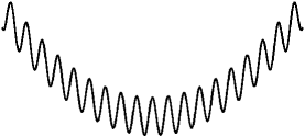
Figure 1: Schematic diagram showing the combined harmonic lattice potential considered in this paper.

We also note several studies showing how adiabatic variations of the lattice depth might be used to prepare a condensate or reversibly condense the system Olshanii and Weiss (2002); Blakie and Porto (2004) and recent papers debating the use of interference peaks as a signature of condensation Diener et al. (2007); Gerbier et al. (2007); Yi et al. (2007).

The central difficulty in calculating the properties of a quantum gas in the combined potential is that the spectrum has a rich and complex structure. Several articles have considered aspects of this system Hooley and Quintanila (2004); Viverit et al. (2004); Rigol and Muramatsu (2004); Rey et al. (2005) for the case of one or two spatial dimensions. The first study we are aware of is a tight-binding description of ultra-cold bosons by Polkovnikov et al. Polkovnikov et al. (2002). Refs. Hooley and Quintanila (2004); Rigol and Muramatsu (2004) have made detailed studies of the combined potential spectrum (also within a tight-binding description), and more recently closed-form solutions were given by Rey et al. Rey et al. (2005). In Refs. Viverit et al. (2004); Ruuska and Törmä (2004) an ideal gas of fermions in a 1D combined potential was examined without making the tight-binding approximation. All of these studies have confirmed that, for appropriate parameter regimes, parts of the single particle spectrum will contain localized states. This is in contrast to the translationally invariant system, where inter-atomic interactions or disorder are needed for localization to occur (e.g. see Jaksch et al. (1998); Buonsante et al. (2007)). Experiments with ultra-cold (though non-condensed) bosons Ott et al. (2004) have provided evidence for these localized states.

In this paper we present a theory for an ideal Bose gas in a three dimensional combined harmonic lattice potential. Our treatment includes excited bands, and is thus valid at high temperatures where tight-binding descriptions fail. Central to our approach is the division of the spectrum into two regions: (1) A low energy region consisting of extended oscillator-like states, modified from those of the harmonic potential by the low energy effective mass. (2) A high energy region containing localized states that have an energy related to the local potential energy, and also includes modes in the first vibrational excited bands. The division between these regions is made by the use of an effective Debye energy for the system.

In current experiments with optical lattices inter-particle interactions are typically important, at least in determining the near zero temperature manybody ground state. Interaction effects near the critical region have yet to be examined for the combined potential (although the quasi-1D case is examined in Wild et al. (2006)), and our ideal gas results will be a useful basis for comparison with future studies.

We begin in Section II by introducing relevant energy scales and describe an approximate analytic spectrum and density of states in the combined potential. In Sec. III we compare our analytic density of states to the results of full numerical calculations to justify the validity regime of our analytic approach. We then derive an analytic approximation to the critical temperature in the combined potential and calculate corrections resulting from the low energy spectrum and the effects of excited bands. Those results are compared to full numerical calculations to assess their accuracy and validity. Finally in Sec. IV we present some general numerical results for the condensation phase diagram in the combined potential. We show how varying the harmonic confinement can be used to raise or lower the transition temperature relative to the pure harmonically trapped case.

II Formalism

II.1 Single particle Hamiltonian

We consider the case of a single particle Hamiltonian of the form

$$H=\frac{p^{2}}{2m}+\sum_{j=1}^{3}\left[V_{j}\sin^{2}\left(\frac{bx_{j}}{2}\right)+\frac{1}{2}m\omega_{j}^{2}x_{j}^{2}\right],$$ (1)

where $b$ is the reciprocal lattice vector, and $\{V_{1},V_{2},V_{3}\}$ are the lattice depths in each direction. It is conventional to define the recoil energy $E_{R}=\hbar\omega_{R}=h^{2}/8ma^{2}$ as an energy scale for specifying the lattice depth, where $a=2\pi/b$ is the direct lattice vector. Properties of the single particle spectrum have been discussed by several authors, e.g. see Refs. Blakie et al. (2007); Rey et al. (2005); Rigol and Muramatsu (2004); Hooley and Quintanila (2004); Viverit et al. (2004). Here we use the results of these studies to suggest an approximate (piecewise) analytic density of states for the combined lattice appropriate for determining the critical temperature.

We begin in the next subsection by defining a set of useful quantities that will be crucial for developing approximations to the spectrum in different regimes. These quantities can be determined from solutions of the much simpler translationally invariant lattice (i.e. Eq. (1) with all $\omega_{j}=0$) or from analytic approximations valid in the tight-binding regime.

II.2 Energy scales from the translationally invariant lattice

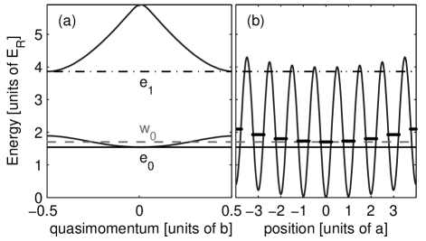
Figure 2: Schematic diagram of important energy scales. (a) Band structure of a translationally invariant 1D lattice of depth $4E_{R}$. Energy scales $e_{0}$ (black horizontal line) , $w_{0}$ (grey dashed line) and $e_{1}$ (dash-dot line) identified (see text). (b) Correspondence of these energy scales to the combined potential. Small thick horizontal lines indicate the energies of ground band localized states.

A one-dimensional depiction of the important energy scales is given in Fig. 2. There we show the one dimensional band structure [Fig. 2(a)], and indicate several energies that we discuss further below.

II.2.1 Bloch state parameters

The quantity $e_{n}$ refers to the minimum (Bloch state) energy of the band with $n$-vibrational quanta, and in the full 3-dimensional case we will use the notation $e_{nj}$ to denote the particular $n$-th excited band by specifying additional quantum number(s) $j$. Here we will only refer to a few of these band minimum energies: $e_{0}$ is the ground state energy of the translationally invariant lattice and gives a lower bound for the ground state energy when the harmonic trap is added; $e_{1j}$ is the lowest energy of the first vibrational excited state, with the quantum number $j=1,2,3$ used indicate that the vibrational excitation is directed along the $x_{j}$-direction; We use $e_{2}$ to indicate the energy above which higher excited bands become accessible .

II.2.2 Wannier state parameters

We define $w_{0}$ as the energy of a localized Wannier state in the ground band. Wannier states are defined as a Fourier transform of the ground band Bloch states (e.g. see Jaksch et al. (1998); Blakie and Clark (2004)), and as such its energy is the mean energy of all the ground band Bloch states (see Fig. 2(a)). The tunneling between neighbouring Wannier states in the $x_{j}$-direction is characterized by the tunneling matrix element $J_{j}$. This is given by the Fourier transform of the ground band Bloch dispersion relation along direction $x_{j}$.

II.2.3 Effective mass

Intermediate between the extended Bloch states and localized Wannier states we will need to describe finite extent wavepackets in the ground band. A convenient quantity for doing this is the effective mass at zero quasimomentum, $m_{j}^{*}$, defined as

$$\frac{1}{m_{j}^{*}}=\frac{1}{\hbar^{2}}\left(\frac{\partial^{2}e_{0}(\mathbf{q})}{\partial q_{j}^{2}}\right)_{\mathbf{q=0}},$$ (2)

where $e_{0}(\mathbf{q})$ is the dispersion relation of the ground band and $\mathbf{q}$ is the quasimomentum. We note that the effective mass may be different along each direction.

II.2.4 Tight-binding expressions

All of the above quantities are easily obtained from calculations of the translationally invariant lattice or equivalently from the well-known properties of the Matthieu functions. However the tight-binding limit, which should be applicable when $V_{j}\gtrsim 5E_{R}$, yields several simple analytic expressions for these quantities. In the appendix of Ref. Blakie et al. (2007) an approximation for the energies of the excited bands is developed using a harmonic oscillator approximation. Using those results we obtain $e_{0}\approx\left(\sum_{j}\sqrt{V_{j}E_{R}}\right)-\frac{3}{4}E_{R},$ $e_{1j}\approx(2\sqrt{V_{j}E_{R}}-E_{R})+e_{0}$, and $e_{2}\approx 4\sqrt{\min\{V_{j}\}E_{R}}-3E_{R}+e_{0}.$ The tunneling matrix element can also be calculated using the harmonic oscillator approximation, giving $J_{j}\approx(4/\sqrt{\pi})(V_{j}/E_{R})^{3/4}\exp(-2\sqrt{V_{j}/E_{R}})E_{R}$. In the tight-binding limit the ground band dispersion relation is approximately given by $e_{0}(\mathbf{q})=\sum_{j}4J_{j}\sin^{2}(q_{j}a/2)+e_{0},$ where $\mathbf{q}$ is the quasimomentum. From this we obtain expressions for the Wannier energy $w_{0}=e_{0}+\sum_{j}2J_{j}$, and the effective mass $m_{j}^{*}=\hbar^{2}/2J_{j}a^{2}$.

II.3 Spectrum and density of states in the combined harmonic lattice potential

II.3.1 Low energy spectrum ($\epsilon<E_{{\rm LE}}$)

The low energy states in the lattice are extended wavepackets, with a harmonic oscillator envelope. Indeed, the spectrum is that of a harmonic oscillator but with the frequency modified by the effective mass, $\omega_{j}^{*}=\sqrt{m/m_{j}^{*}}\omega_{j}$ Rey et al. (2005), i.e.

$$\epsilon_{{\rm LE}}(\mathbf{n})=e_{0}+\sum_{j=1}^{3}\hbar\omega_{j}^{*}\left(n_{j}+\frac{1}{2}\right),$$ (3)

where the $\{n_{j}\}$ are non-negative integers. This low energy description is valid for quantum numbers in the range $0\leq n_{j}\leq\mathcal{N}_{j}$ where

$$\mathcal{N}_{j}\equiv 4\sqrt{J_{j}/m\omega_{j}^{2}a^{2}},$$ (4)

(see Rey et al. (2005)) as for values of $n_{j}$ greater than $\mathcal{N}_{j}$ the states become localized (see below).

The density of states for these modes is given by

$$g_{{\rm LE}}(\epsilon)=\frac{(\epsilon-e_{0})^{2}}{2\hbar^{3}\overline{\omega^{*}}^{3}},\quad e_{0}\leq\epsilon<E_{{\rm LE}},$$ (5)

where $\overline{\omega^{*}}=\sqrt[3]{\omega_{1}^{*}\omega_{2}^{*}\omega_{3}^{*}}$ is the geometric mean of the effective trap frequencies. The boundary of the rectangular region of $\{n_{j}\}$-space, where the low energy description is valid, does not correspond to a well-defined energy cutoff. We introduce an effective Debye energy, $E_{{\rm LE}}$, such that a total of $\mathcal{N}_{1}\mathcal{N}_{2}\mathcal{N}_{3}$ low energy states would lie below this energy. A simple calculation yields

$$E_{{\rm LE}}=4\sqrt[3]{6}\hbar\sqrt{\frac{\bar{J}}{\overline{m^{*}}a^{2}}}+e_{0},$$ (6)

where $\bar{J}$ and $\overline{m^{*}}$ are the geometric means of the tunneling matrix elements ($J_{j}$) and effective masses ($m_{j}^{*}$) respectively. Since $E_{{\rm LE}}$ depends on $\bar{J}$ it is exponentially suppressed towards $e_{0}$ as the lattice depth increases.

The ground state energy of the combined potential, corresponding to the state in which the condensate forms, is given by Eq. (3) with $n_{1}\!=\!n_{2}\!=\!n_{3}\!=\!0,$ i.e.

$$\epsilon_{g}=e_{0}+\frac{1}{2}\sum_{j}\hbar\omega_{j}^{*}.$$ (7)

We see that the effect of the harmonic confinement is to shift the ground state energy upward from that of the translationally invariant lattice i.e, $e_{0}$. However, $\epsilon_{g}$ will still be less than $w_{0}$ if the harmonic potential is less confining than a single lattice site.

II.3.2 Localized spectrum ($\epsilon\geq E_{{\rm LE}}$)

The next part of the spectrum consists of localized states, arising because the offset in potential energy between lattice sites near the classical turning point exceeds the respective tunneling matrix element. The nature of these states and the derivation of their respective density of states is treated fully in Ref. Blakie et al. (2007), but we briefly summarize those results here.

The energies of the localized states are given by the local potential energy

$$\epsilon_{{\rm L}0}(\mathbf{n})=\frac{1}{2}ma^{2}(\omega_{1}^{2}n_{1}^{2}+\omega_{2}^{2}n_{2}^{2}+\omega_{3}^{2}n_{3}^{2})+w_{0},$$ (8)

where $\{n_{j}\}$ are (positive and negative) integers that specify the site where the state is localized. As these states localize to approximately a single lattice site, their energy offset from the lattice site minimum (i.e. $\frac{1}{2}ma^{2}\sum_{j}\omega_{j}n_{j}^{2}$) is given by the Wannier energy $w_{0}$. Schematically these states are indicated in Fig. 2(b) as horizontal rungs in each lattice site (recalling that for $\epsilon_{{\rm L0}}(\mathbf{n})\lesssim E_{{\rm LE}}$ tunneling delocalizes these states).

This description is valid for all energies above $E_{{\rm LE}}$, however for sufficiently high energy scales additional vibrational states become available. Here we will also approximate these excited band states using a localized description, i.e.

$$\epsilon_{{\rm L}1j}(\mathbf{n})=\frac{1}{2}ma^{2}(\omega_{1}^{2}n_{1}^{2}+\omega_{2}^{2}n_{2}^{2}+\omega_{3}^{2}n_{3}^{2})+e_{1j},\quad j=1,2,3$$ (9)

where we have approximated the zero point energy of these states as $e_{1j}$. Note that because the vibrational excitation may be directed along any coordinate direction we have three first excited bands to include.

The density of states for the spectra given in Eqs. (8) and (9) is

$$g_{{\rm Loc}}(\epsilon)=g_{0}(\epsilon-w_{0})+\sum_{j=1}^{3}g_{0}(\epsilon-e_{1j}),\quad E_{{\rm LE}}\leq\epsilon<e_{2},$$ (10)

where

$$g_{0}(\epsilon)=\frac{16}{\pi^{2}}\left(\frac{\omega_{R}}{\hbar\bar{\omega}^{2}}\right)^{3/2}\sqrt{\epsilon}\,\theta(\epsilon),$$ (11)

$\bar{\omega}=\sqrt[3]{\omega_{1}\omega_{2}\omega_{3}}$, (e.g. see Blakie et al. (2007); Köhl (2006)), and $\theta(\epsilon)$ is the unit step function. We also note that the case of a general (non-separable lattice) has the same density of states if we instead identify $E_{R}=h^{2}/8mV_{c}^{2/3},$ where $V_{c}=|\mathbf{a}_{1}\cdot(\mathbf{a}_{2}\times\mathbf{a}_{3})|$ is the unit cell volume and $\{\mathbf{a}_{1},\mathbf{a}_{2},\mathbf{a}_{3}\}$ are the direct lattice vectors.

The localized states description of the first excited band is the most severe approximation we make for the combined potential spectrum, particularly because the lowest energy states of the excited bands will also be harmonic oscillator-like. For deep lattices the tunneling rates for the ground and excited bands are small and the localized description improves. For the theory we develop here, the first excited bands are assumed to be a rather large energy scale compared to the critical temperature and this approximation should be adequate.

II.3.3 Bare oscillator states ($\epsilon>E_{{\rm bare}}$)

At sufficiently high energy scales the lattice has only a small effect on the energy eigenstates and the spectrum crosses over to bare oscillator states. This cross-over occurs when the single particle energies exceed the lattice depth which in 3D we can take as the sum of the lattice coefficients $E_{{\rm bare}}=\sum_{j}V_{j}$. The bare oscillator spectrum is of the form given in Eq. (3) but with the bare trap frequencies, i.e.

$$\epsilon_{{\rm bare}}(\mathbf{n})=\epsilon_{V}+\sum_{j=1}^{3}\hbar\omega_{j}\left(n_{j}+\frac{1}{2}\right),$$ (12)

where $n_{j}$ are non-negative integers. The constant $\epsilon_{V}=\frac{1}{2}\sum_{j=1}^{3}V_{j}$ is the spatial average of the lattice potential and gives the shift of the high energy spectrum. The density of states is given by

$$g_{{\rm bare}}(\epsilon)=\frac{(\epsilon-\epsilon_{V})^{2}}{2\hbar^{3}\bar{\omega}^{3}},\quad\epsilon>E_{{\rm bare}}.$$ (13)

For the parameter regimes of interest (lattices with depths greater than a few recoils) $E_{{\rm bare}}$ is sufficiently large that the bare oscillator states do not play an important role in determining the condensation properties for the system.

II.3.4 Intermediate energy region

In sufficiently deep lattices many excited bands may be bound by the lattice, and will contribute to the density of states. In this case for energies greater than $e_{2}$ and less than $E_{{\rm bare}}$, the various density of states we have already outlined above will be inadequate. It is difficult to provide a reliable analytic description of these excited band contributions for several reasons: (1) Anharmonic effects of the lattice make predicting the locations (i.e. $e_{nj}$) of these bands difficult. (2) The tunneling between sites in excited bands is much larger and worsens the localized state approximation. This necessitates an effective mass modified harmonic oscillator treatment (c.f. Eq. (3)) that crosses over to localized states at higher energies. Furthermore, large asymmetry between directions can occur depending on the orientation of the vibrational excitations of each band, making any form of Debye approximation of limited use.

Here we do not treat these higher bands analytically. For typical experimental parameters the energy scale of these modes (i.e. $e_{2}$) is well above $kT_{c}$, and a complete description is not required.

II.4 Full numerical solution

To test the predictions of this paper we have made a full numerical solution for the single particle eigenstates of Eq. (1). To do this we use the separability of the Hamiltonian to convert this eigenvalue problem to a set of three 1D problems. Because the harmonic potential is quite weak (typically $\omega_{j}\sim 0.01-0.05\omega_{R}$ in experiments), a large number of lattice sites need to be represented to find eigenstates up to a convenient maximum energy (usually $E_{\max}\approx\epsilon_{g}+25E_{R}$), chosen so that the density of states we construct will be useful for temperatures up to about $T\sim 5E_{R}/k$. We use a planewave decomposition to represent the eigenstates of the combined potential, chosen because it provides an efficient representation of the rapidly varying lattice potential. Typically of order $10^{4}-10^{5}$ planewave modes are used to represent the several thousand eigenstates in the energy range of interest.

For the purposes of comparison to our analytic results, it is useful to construct a smoothed density of states, defined as

$$\bar{g}(\epsilon)=\frac{1}{2\Delta\epsilon}\int_{\epsilon-\Delta\epsilon}^{\epsilon+\Delta\epsilon}d\epsilon\,\sum_{ijk}\delta(\epsilon-[\epsilon_{i}^{(1)}+\epsilon_{j}^{(2)}+\epsilon_{k}^{(3)}]),$$ (14)

that gives an average number of eigenstates per unit energy with energies lying within $\Delta\epsilon$ of $\epsilon$, where $\{\epsilon_{i}^{(j)}\}$ are the (1D) single particle energies ($i=0,1,\ldots$) in the $x_{j}$- direction obtained form the numerical diagonalization.

III Results

III.1 Density of states

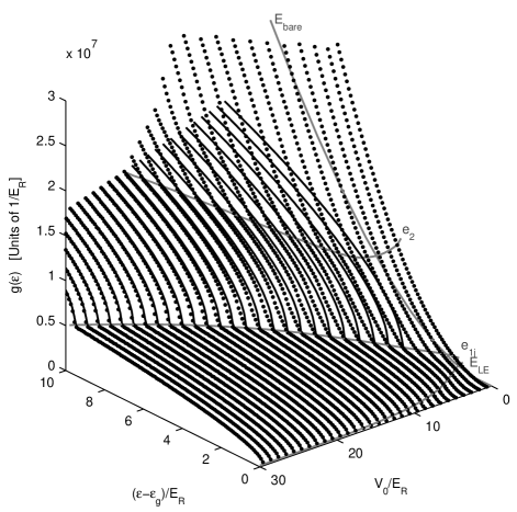
Figure 3: Comparison of numerical smoothed density of states $\bar{g}(\epsilon)$ (dots) to analytic density of states $\tilde{g}(\epsilon)$ (black lines) for a 3D combined harmonic lattice potential. The lattice depth parameters are the same for each direction, i.e. $V_{j}=V_{0}$ for $j=1,2,3$. For reference, the characteristic energy scales $E_{{\rm LE}}$ , $e_{1j}$, $e_{2}$ and $E_{{\rm bare}}$ are shown as gray curves. Isotropic harmonic trap taken with $\bar{\omega}=0.01\omega_{R}$. All energies are measured relative to $\epsilon_{g}$.

Here we investigate the accuracy and applicability of our combined density of states (5) and (10) by comparison with the smoothed density of states obtained from the full numerical solution (see Fig. 3). For definiteness, the analytic density of states we use is constructed piecewise from results (5) and (10), as

$$\tilde{g}(\epsilon) = \left\{\begin{array}[]{cc}g_{{\rm LE}}(\epsilon)&e_{0}<\epsilon<E_{{\rm LE}},\\ g_{{\rm Loc}}(\epsilon)&E_{{\rm LE}}\leq\epsilon.\end{array}\right.$$ (17)

Of course this result can only be expected to furnish a good description for $\epsilon\lesssim e_{2}.$ In the context of current experiments this energy range should be sufficiently large that this piecewise density of states will be useful over a broad parameter regime. E.g. for ⁸⁷Rb in a $10E_{R}$ deep lattice ($a=425$nm), we have that $(e_{2}-e_{0})\sim 10E_{R}\sim k\times 1.5\mu$K.

We make a few observations regarding the results in Fig. 3:

1. For shallow lattices $E_{{\rm bare}}$ may be sufficiently small that the transition to bare oscillator states occurs before $E_{{\rm LE}}$ is reached. Indeed, the density of states is mostly harmonic oscillator like (i.e. $\bar{g}\sim\epsilon^{2}$) for lattice depths less than $4E_{R}$, and for this reason the analytic result is only shown for depths greater than this.

2. For lattice depths less than $10E_{R}$ the onset of the localized excited band states in $\tilde{g}(\epsilon)$ for $\epsilon\sim e_{1j}$ is too rapid compared to the numerical results, arising because the lowest energy states in the excited band are harmonic oscillator like. However, agreement is observed to improve with increasing lattice depth, such that for $V_{0}\gtrsim 20E_{R}$ the numerical and analytic results are almost indistinguishable.

3. The energy scale $e_{2}$ increases quite rapidly with lattice depth, justifying our neglect of additional excited bands in the analytic density of states.

III.2 Analytic prediction for the critical temperature

As is apparent from Fig. 3, for lattices with $V_{j}\gtrsim 4E_{R}$, the majority of the low energy spectrum is well described by the first term of the localized density of states (10), and thus we use this term to estimate the critical temperature.

The total number of particles in the ground band localized states, as a function of inverse temperature ($\beta=1/kT$ ) and chemical potential ($\mu$), is given by

$$N_{{\rm Loc}}(\beta,\mu) = \int_{w_{0}}^{\infty}d\epsilon\,\frac{g_{0}(\epsilon-w_{0})}{e^{\beta(\epsilon-\mu)}-1},$$ (18)

$$= \frac{16}{\pi^{2}}\left(\frac{kT\,\omega_{R}}{\hbar\bar{\omega}^{2}}\right)^{\frac{3}{2}}\!\Gamma\left(\!\frac{3}{2}\!\right)g_{\frac{3}{2}}\left(e^{\beta(\mu-w_{0})}\right),$$ (19)

where $g_{s}(z)=\sum_{k=1}^{\infty}z^{k}/k^{s}$ is the polylogarithm function.

Following the usual procedureHuang (1987) we identify the critical temperature for condensation by taking the gas to be saturated ($\mu\to w_{0}$) and setting $N_{{\rm Loc}}(\beta_{c0},w_{0})=N$ (the total number of atoms), giving

$$T_{c0}\approx\frac{0.4141}{k}\left(\frac{\hbar\bar{\omega}^{2}}{\omega_{R}}\right)N^{2/3},$$ (20)

where $\beta_{0c}=1/kT_{c0}$ and we have used that $g_{3/2}(1)=\zeta(3/2)\approx 2.612$, with $\zeta(s)=\sum_{k=1}^{\infty}1/k^{s}$ the Reimann zeta function. This expression has the same $N^{2/3}$ dependence as the critical temperature for the uniform Bose gas.

III.3 Corrections to analytic critical temperature

Expression (20) for $T_{c0}$ is based solely on the localized ground band states. The effect of the low energy states (5) and excited band states (10) are in general significant. We now consider the effect of these on $T_{c0}$ under the assumptions that $(E_{{\rm LE}}-e_{0})/kT_{c0}\ll 1$ and $(e_{2}-e_{0})/kT_{c0}\gg 1$.

III.3.1 Low energy correction

The first correction we consider is to account for the low energy spectrum, described in Sec.II.3.1. To do this we replace $g_{0}(\epsilon-w_{0})$ in (18) for $\epsilon<E_{{\rm LE}}$ by the low energy density of states (5). This changes $N_{{\rm Loc}}(\beta_{c0},\mu)$ by an amount

$$\Delta N_{{\rm LE}} = \int_{\epsilon_{0}}^{E_{{\rm LE}}}d\epsilon\,\frac{g_{{\rm LE}}(\epsilon)}{e^{\beta_{c0}(\epsilon-e_{0})}-1}-\int_{w_{0}}^{E_{{\rm L}E}}d\epsilon\,\frac{g_{0}(\epsilon-w_{0})}{\epsilon^{\beta_{c0}(\epsilon-w_{0})}-1},$$ (21)

$$\approx kT_{c0}\left[\frac{(E_{{\rm LE}}-e_{0})^{2}}{4\left(\hbar\overline{\omega^{*}}\right)^{3}}-\frac{32}{\pi^{2}}\left(\frac{\omega_{R}}{\hbar\bar{\omega}^{2}}\right)^{3/2}\sqrt{E_{{\rm LE}}-w_{0}}\right]$$ (22)

where we have assumed that $(E_{{\rm LE}}-e_{0})\ll kT_{c0}$ to arrive at the last line .

III.3.2 Chemical potential correction

Associated with the change in the low energy density of states is the change in ground state energy from $w_{0}$ (for the localized spectrum) to $\epsilon_{g}$ (for the low energy spectrum (7)). Replacing the saturated chemical potential by the ground state energy, i.e. setting $\mu\to\epsilon_{g}$ in (19) we obtain

$$\Delta N_{{\rm\mu}}=\frac{-32}{\pi^{3/2}}\left(\frac{\omega_{R}}{\hbar\bar{\omega}^{2}}\right)^{3/2}\sqrt{w_{0}\!-\!\epsilon_{g}}\left(1\!+\!\frac{\zeta(\frac{1}{2})}{2}\sqrt{\frac{w_{0}-\epsilon_{g}}{\pi kT_{c0}}}\right)kT_{c0}.$$ (23)

In deriving this result we have assumed that $(w_{0}-\epsilon_{g})/kT_{c0}\ll 1,$ so that we can approximate the argument of the polylogarithm as $1-(w_{0}-\epsilon_{g})/kT_{0c}$, and use the expansion $g_{3/2}(1-x)\approx\zeta(3/2)-2\sqrt{\pi x}-\zeta(1/2)x.$ We note that $\zeta(\frac{1}{2})\approx-1.460$ and the square root term accounts for the infinite slope of $g_{3/2}(z)$ at $z=1$.

III.3.3 Excited band correction

As discussed in the derivation of Eq. (10), at an energy scale of $e_{1j}$ excited band states become accessible to the system, and contribute additional states described by the density of states $g_{0}(\epsilon-e_{1j})$ . The additional atoms accommodated in these states at $T_{c0}$ is given by

$$\Delta N_{{\rm EB}} = \sum_{j=1}^{3}\int_{w_{1j}}^{\infty}d\epsilon\,\frac{g_{0}(\epsilon-e_{1j})}{\epsilon^{\beta_{c0}(\epsilon-w_{0})}-1},$$

$$\approx \sum_{j=1}^{3}\frac{8}{\pi^{3/2}}\left(\frac{kT_{c0}\omega_{R}}{\hbar\bar{\omega}^{2}}\right)^{3/2}e^{-(e_{1j}-w_{0})/kT_{c0}},$$

where we have taken $(e_{1j}-w_{0})\gg kT_{c0}$. Note that in calculating this term we have summed over all contributing first excited bands.

III.3.4 Corrected critical temperature

Combining all the above results we arrive at a new estimate for the transition temperature. To do this we set

$$N=N_{{\rm Loc}}(\beta_{c1},w_{0})+\Delta N_{{\rm LE}}+\Delta N_{\mu}+\Delta N_{{\rm EB}},$$ (25)

where $\beta_{c1}=1/kT_{c1}$ is the corrected transition temperature. Assuming that $|T_{c1}-T_{c0}|\ll T_{c0}$, we obtain

$$T_{c1}\approx T_{c0}\left[1-\frac{2}{3}(\Delta N_{{\rm LE}}+\Delta N_{{\rm\mu}}+\Delta N_{{\rm EB}})/N\right],$$ (26)

to first order in the $\Delta N$-corrections. The validity conditions are, as stated above, that $(E_{{\rm LE}}-e_{0})/kT_{c0}\ll 1$ and $(e_{2}-e_{0})/kT_{c0}\gg 1$. This will ensure that all the changes ($\Delta N$) are small compared to $N$, however we caution that sometimes due to cancellation a particular $\Delta N$ can be small even when the validity condition is not satisfied.

We make the following observations on these corrections:

• The low energy density of states tends to increase much more slowing from its zero point than the localized density of states does. Thus in replacing $g_{0}(\epsilon)$ by $g_{{\rm LE}}(\epsilon)$ in (18), the number of states at low energy and hence the number of atoms in the saturated thermal cloud both decrease. This leads to an increase in the critical temperature.

• The downward shift of the chemical potential when we change the saturated chemical potential from $w_{0}$ to $\epsilon_{g}$ leads to a decrease in the number of atoms in the saturated thermal cloud, and hence an increase in the critical temperature.

• Including higher bands brings additional states and hence increases the number of atoms in the saturated thermal cloud. This has the effect of decreasing the critical temperature.

Interestingly the dominant corrections at low temperatures ($\Delta N_{{\rm LE}}$ and $\Delta N_{{\rm\mu}}$) both lead to an increase in $T_{c}$, whereas the dominant correction at higher temperatures ($\Delta N_{{\rm EB}}$) shifts $T_{c}$ downwards.

III.4 Numerical calculations of $T_{c}$

While the analytic calculation provides a useful critical temperature estimate, the complexity of the spectrum in the combined harmonic-lattice potential necessitates a numerical solution. Here we discuss our procedure for calculating the critical temperature using the spectrum determined by full numerical diagonalization of (1) and give a simple numerical scheme that makes use of the piecewise density of states we have developed in Secs. II.3.1 and II.3.2.

III.4.1 Full numerical calculation

From the results of our full diagonalization we determine the one-dimensional energy spectrum $\{\epsilon_{i}^{(j)}\}$ over a large energy range, typically including all states up to energy $25E_{R}$ above the 1D ground state energy (as discussed in Sec. II.4). The thermal properties of the system are then calculated over a temperature range by iterating the chemical potential $\mu$ to find the desired total number of atoms, i.e. root-finding the expression$f(\mu)=\left[\sum_{ijk}\{\exp([\epsilon_{i}^{(1)}+\epsilon_{j}^{(2)}+\epsilon_{k}^{(3)}-\mu]/kT)-1\}^{-1}-N\right]$ for each $T.$ From this calculation we hence evaluate the condensate population as a function of temperature, i.e, $N_{0}(T)=\{\exp([\sum_{j=1}^{3}\epsilon_{0}^{(j)}-\mu]/kT)-1\}^{-1}$, and determine the condensation temperature as that at which $|(\partial N_{0}/\partial T)/N_{0}|$ (i.e. the relative change in the ground state occupation) is maximised.

III.4.2 Simple numerical calculation

The critical temperature can also be estimated by performing a simple numerical integral using the piecewise analytic density of states (17) under the saturated thermal cloud condition ($i.e.$ $\mu\to e_{0}$)

$$N(T)=\int_{e_{0}}^{E_{\max}}d\epsilon\frac{\tilde{g}(\epsilon)}{e^{(\epsilon-e_{0})/kT}-1}.$$ (27)

This result can then be numerically inverted to give a critical temperature estimate $T_{cN}=T_{cN}(N).$ The energy $E_{\max}$ appearing in the integral has to be chosen such that $E_{\max}\gg kT$, in which case the result will be independent of $E_{\max}$.

This approach is significantly simpler than the full numerical calculation because it does not require a full numerical diagonalization. Indeed the information needed for $\tilde{g}(\epsilon)$ can be obtained from results of the uniform lattice or tight-binding approximations, as discussed in Sec. II.2.

III.5 Comparison of analytic and numerical critical temperatures

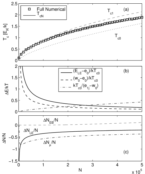
Figure 4: Comparison of analytic and numerical critical temperatures (a) Full numerical results for $T_{c}$ (squares), analytic results $T_{c0}$ (dotted), $T_{c1}$ (dashed) and simple numerical result using piecewise analytic density of states $T_{cN}$ (solid). (b) Energy scales compared to $T_{c0}$. (c) $\Delta N$-corrections. Calculation parameters: isotropic harmonic trap with $\bar{\omega}=0.025\omega_{R}$, and lattice depth parameters $V_{j}=8E_{R}$ for $j=1,2,3$.

In Fig. 4(a) we show analytic and numerical results for the critical temperature. To relate these parameters to those in experiment we note that for ⁸⁷Rb in a lattice with $a=425$nm, the trap frequency corresponds to $\omega\approx 2\pi\times 31\,s^{-1}$ while the temperature scale is $E_{R}/k\approx 152nK$. These results show the general behaviour we have observed over a wide parameter regime. $T_{c0}$ provides a useful critical temperature estimate, though is noticeably shifted relative to the full numerical result. Including first order corrections $T_{c1}$ provides a quantitatively much more accurately result, although its agreement with the full numerical result worsens for large $N$. Interestingly the simple numerical result $T_{cN}$ outlined in Sec. III.4.2 provides an accurate description over the full range considered.

In Fig. 4(b) and (c) we explore the validity conditions for our derivation of the critical temperature. Note for the potential parameters used for the results in Fig. 4 we have that $E_{{\rm LE}}-e_{0}=0.304E_{R}$, $E_{{\rm LE}}-w_{0}=0.123E_{R}$, $e_{1j}-w_{0}=3.83E_{R}$, and $e_{2}-e_{0}=6.7E_{R}$. The relative size of the parameters $(E_{{\rm LE}}-e_{0})/kT_{c0}$, $(E_{{\rm LE}}-w_{0})/kT_{c0}$ and $kT_{c0}/(e_{1j}-w_{0})$ are shown in Fig. 4(b). We require all of these parameters to be small for our analytic calculation to be valid. These results show that for small $N$ the critical temperature is sufficiently low that a first order treatment of the low energy spectrum is not appropriate (i.e. both $(E_{{\rm LE}}-e_{0})/kT_{c0}$ and $(E_{{\rm LE}}-w_{0})/kT_{c0}$ are large).

At larger atom numbers ($N$) the term $kT_{c0}/(e_{1j}-w_{0})$ tends to grow reflecting the increased importance of excited band states. In Fig. 4(c) we show the related values of $\Delta N_{{\rm LE}}$, $\Delta N_{\mu}$ and $\Delta N_{{\rm EB}}$. At small $N$ ( and hence small $T_{c0}$) the expansions we have used to obtain$\Delta N_{{\rm LE}}$ and $\Delta N_{\mu}$ are not valid. As $N$ increases these contributions become less significant relative to $N,$ however as $\Delta N_{\mu}$ scales like $\sqrt{(E_{{\rm LE}}-w_{0})/kT_{c0}}$ it decreases rather slowly with increasing $T_{c0}$. Finally, the excited band contribution becomes gradually more significant with increasing number.

IV General behaviour of condensation in the combined potential

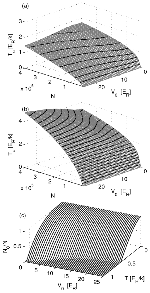
Figure 5: Bose-Einstein condensation in a combined harmonic lattice potential. (a) Critical temperature as a function of lattice depth (all $V_{j}=V_{0}$) and total atom number for an isotropic harmonic trap with $\bar{\omega}=0.025\omega_{R}$. Isothermal levels spaced by $0.2E_{R}/k$ shown as contour lines. (b) As for (a) but with $\bar{\omega}=0.05\omega_{R}$. (c) Condensate fraction versus temperature for the same parameters as (a) and $N=1\times 10^{5}$ atoms.

In figure 5 we show the results of our full numerical calculation (as discussed in Sec. III.4.1) for the critical temperature and condensate fraction over a wide parameter regime. For the case of $\bar{\omega}=0.025\omega_{R}$ in Fig. 5(a) we see that as the lattice depth increases the critical temperature of the system decreases. While for the case of $\bar{\omega}=0.05\omega_{R}$ shown in Fig. 5(b) the critical temperature instead tends to increase with increasing lattice depth (for $N$ sufficiently large).

To understand these results we recall the critical temperature for a harmonically trapped gas

$$T_{{\rm harm}}=\frac{\hbar\bar{\omega}}{k}\left(\frac{2N}{\Gamma(3)\zeta(3)}\right)^{\frac{1}{3}}.$$ (28)

In comparison to our analytic result given in Eq. (20), we note that the critical temperature for the combined potential scales with mean trap frequency and total atom number at higher powers, i.e. $\bar{\omega}^{2}$ and $N^{2/3}$ respectively. Locating the trap frequency at which the critical temperatures for the harmonic and combined potentials are the same determines a critical mean trap frequency ($\bar{\omega}_{c}(N)$):

$$\frac{\bar{\omega}_{c}(N)}{\omega_{R}}=\frac{4}{\pi}\left(\frac{\zeta\left(\frac{3}{2}\right)^{2}}{\zeta(3)}\right)^{\frac{1}{3}}\frac{1}{\sqrt[3]{N}}.$$ (29)

For $\bar{\omega}>\bar{\omega}_{c}$ the critical temperature is higher in the combined potential than for the pure harmonic trap, whereas for $\bar{\omega}<\bar{\omega}_{c}$ the pure harmonic potential has a higher critical temperature. For $N=10^{5}$ atoms we find that $\bar{\omega}_{c}\sim 0.049\omega_{R}$, which is consistent with Figs. 5(a) and 5(b) which lie either side of this value. Since $\bar{\omega}_{c}$ is based on the simple critical temperature estimate (20), it will only be valid for cases where the critical temperature is not too high or low (as given by the validity conditions in Sec. III.3).

In Fig. 5(c) we show the condensate fraction versus temperature for a system of $10^{5}$ atoms in a combined potential with $\bar{\omega}=0.025\omega_{R}$. As the lattice depth increases the critical temperature shifts downwards (as can also be discerned from Fig. 5(a)), and the characteristic shape of the condensate fraction dependence on temperature, $N_{0}\sim[1-(T/T_{c})^{\alpha}]$, changes from $\alpha\sim 3$ to $\alpha\sim 3/2$. These predicted features should be verifiable by current experiments.

V Conclusion

We have performed a comprehensive study of the critical temperature for an ideal Bose gas in a combined harmonic lattice potential. We have described distinctive regions of the spectrum and have shown that a simple piecewise density of states provides an accurate characterization of this system for lattice depths greater than about $4E_{R}$. We have developed an analytic expression for the critical temperature in the combined potential. The corrections to this result are typically significant, and we have shown that including them provides a useful estimate for the critical temperature obtained by a full numerical calculation. Additionally, we give a simple numerical procedure based on piecewise density of states that provides an accurate prediction for the critical temperature. Finally we have presented results over a wide parameter regime appropriate to current experiments and have shown that the critical temperature in the combined potential can be increased or decreased relative to that of the pure harmonic trap.

References

- Anderson and Kasevich (1998) B. Anderson and M. Kasevich, Science 282, 1686 (1998).
- Burger et al. (2001) S. Burger, F. Cataliotti, C. Fort, F. Minardi, M. Inguscio, M. Chiofalo, and M. Tosi, Phys. Rev. Lett. 86, 4447 (2001).
- Greiner et al. (2002a) M. Greiner, O. Mandel, T. W. Hänsch, and I. Bloch, Nature 419, 51 (2002a).
- Hensinger et al. (2001) W. K. Hensinger, H. Haffner, A. Browaeys, N. R. Heckenberg, K. Helmerson, C. McKenzie, G. J. Milburn, W. D. Phillips, S. L. Rolston, H. Rubinsztein-Dunlop, et al., Nature 412, 52 (2001).
- Morsch et al. (2003) O. Morsch, J. H. Müller, D. Ciampini, M. Cristiani, P. B. Blakie, C. J. Williams, P. S. Julienne, and E. Arimondo, Phys. Rev. A 67, 031603 (2003).
- Orzel et al. (2001) C. Orzel, A. K. Tuchman, M. L. Fenselau, M. Yasuda, and M. A. Kasevich, Science 23, 2386 (2001).
- Spielman et al. (2006) I. Spielman, P. R. Johnson, J. Huckans, C. Fertig, S. Rolston, W. Phillips, and J. Porto, Phys. Rev. A 73, 020702 (2006).
- Greiner et al. (2002b) M. Greiner, O. Mandel, T. Esslinger, T. W. Hänsch, and I. Bloch, Nature 415, 39 (2002b).
- Jaksch et al. (1998) D. Jaksch, C. Bruder, J. I. Cirac, C. Gardiner, and P. Zoller, Phys. Rev. Lett. 81, 3108 (1998).
- Greiner et al. (2001) M. Greiner, I. Bloch, O. Mandel, T. W. Hänsch, and T. Esslinger, Phys. Rev. Lett. 87, 160405 (2001).
- Morsch et al. (2002) O. Morsch, M. Cristiani, J. H. Müller, D. Ciampini, and E. Arimondo, Phys. Rev. A 66, 021601 (2002).
- Fort et al. (2003) C. Fort, F. S. Cataliotti, L. Fallani, F. Ferlaino, P. Maddaloni, and M. Inguscio, Physical Review Letters 90, 140405 (pages 4) (2003).
- Fertig et al. (2005) C. D. Fertig, K. M. O’Hara, J. H. Huckans, S. L. Rolston, W. D. Phillips, and J. V. Porto, Physical Review Letters 94, 120403 (pages 4) (2005).
- Fallani et al. (2004) L. Fallani, L. D. Sarlo, J. E. Lye, M. Modugno, R. Saers, C. Fort, and M. Inguscio, Phys. Rev. Lett. 93, 140406 (pages 4) (2004).
- Baym et al. (1999) G. Baym, J.-P. Blaizot, M. Holzmann, F. Laloë, and D. Vautherin, Phys. Rev. Lett. 83, 1703 (1999).
- Baym et al. (2001) G. Baym, J.-P. Blaizot, M. Holzmann, F. Laloë, and D. Vautherin, Eur. Phys. J. B 24, 107 (2001).
- Arnold and Moore (2001) P. Arnold and G. Moore, Phys. Rev. Lett. 87, 120401 (2001).
- Kashurnikov et al. (2001) V. A. Kashurnikov, N. V. Prokof’ev, and B. V. Svistunov, Phys. Rev. Lett. 87, 120402 (2001).
- Davis and Morgan (2003) M. J. Davis and S. A. Morgan, Phys. Rev. A 68, 053615 (2003).
- Andersen (2004) J. O. Andersen, Rev. Mod. Phys. 76, 599 (2004).
- Dalfovo et al. (1999) F. Dalfovo, S. Giorgini, L. P. Pitaevskii, and S. Stringari, Rev. Mod. Phys. 71, 463 (1999).
- Giorgini et al. (1996) S. Giorgini, L. P. Pitaevskii, and S. Stringari, Phys. Rev. A 54, R4633 (1996).
- Gerbier et al. (2004) F. Gerbier, J. H. Thywissen, S. Richard, M. Hugbart, P. Bouyer, and A. Aspect, Phys. Rev. Lett. 92, 030405 (2004).
- Zobay et al. (2004) O. Zobay, G. Metikas, and G. Abler, Phys. Rev. A 69, 063615 (2004).
- Davis and Blakie (2006) M. J. Davis and P. B. Blakie, Phys. Rev. Lett. 96, 060404 (2006).
- Kleinert et al. (2004) H. Kleinert, S. Schmidt, and A. Pelster, Phys. Rev. Lett. 93, 160402 (2004).
- Ramakumar and Das (2005) R. Ramakumar and A. N. Das, Phys. Rev. B 72, 094301 (2005).
- Gerbier et al. (2007) F. Gerbier, S. Foelling, A. Widera, and I. Bloch, arXiv:cond-mat/0701420v1 (2007).
- Wild et al. (2006) B. G. Wild, P. B. Blakie, and D. A. W. Hutchinson, Phys. Rev. A 73, 023604 (2006).
- Ramakumar et al. (2007) R. Ramakumar, A. N. Das, and S. Sil, Eur. Phys. J. D 42, 309 (2007).
- Zobay and Rosenkranz (2006) O. Zobay and M. Rosenkranz, Phys. Rev. A 74, 053623 (2006).
- Olshanii and Weiss (2002) M. Olshanii and D. Weiss, Phys. Rev. Lett. 89, 090404 (2002).
- Blakie and Porto (2004) P. B. Blakie and J. V. Porto, Phys. Rev. A 69, 013603 (2004).
- Diener et al. (2007) R. B. Diener, Q. Zhou, H. Zhai, and T.-L. Ho, Phys. Rev. Lett. 98, 180404 (2007).
- Yi et al. (2007) W. Yi, G.-D. Lin, and L.-M. Duan, arXiv:0705.4352 (2007).
- Hooley and Quintanila (2004) C. Hooley and J. Quintanila, Phys. Rev. Lett. 93, 080404 (2004).
- Viverit et al. (2004) L. Viverit, C. Menotti, T. Calarco, and A. Smerzi, Phys. Rev. Lett. 93, 110401 (2004).
- Rigol and Muramatsu (2004) M. Rigol and A. Muramatsu, Phys. Rev. A 70, 043627 (2004).
- Rey et al. (2005) A. M. Rey, G. Pupillo, C. W. Clark, and C. J. Williams, Phys. Rev. A 72, 033616 (2005).
- Polkovnikov et al. (2002) A. Polkovnikov, S. Sachdev, and S. M. Girvin, Phys. Rev. A 66, 053607 (2002).
- Ruuska and Törmä (2004) V. Ruuska and P. Törmä, New J. Phys. 6, 59 (2004).
- Buonsante et al. (2007) P. Buonsante, V. Penna, A. Vezzani, and P. B. Blakie, Phys. Rev. A) 76, 011602 (2007).
- Ott et al. (2004) H. Ott, E. de Mirandes, F. Ferlaino, G. Roati, V. Türck, G. Modugno, and M. Inguscio, Phys. Rev. Lett. 92, 120407 (2004).
- Blakie et al. (2007) P. B. Blakie, A. Bezett, and P. Buonsante, Phys. Rev. A 75, 063609 (2007).
- Blakie and Clark (2004) P. B. Blakie and C. W. Clark, J. Phys. B 37, 1391 (2004).
- Köhl (2006) M. Köhl, Phys. Rev. A 73, 031601(R) (2006).
- Huang (1987) K. Huang, Statistical Mechanics (Wiley, 1987).