Design of Multistage Decimation Filters Using Cyclotomic Polynomials:
Optimization and Design Issues

Abstract

This paper focuses on the design of multiplier-less decimation filters suitable for oversampled digital signals. The aim is twofold. On one hand, it proposes an optimization framework for the design of constituent decimation filters in a general multistage decimation architecture. The basic building blocks embedded in the proposed filters belong, for a simple reason, to the class of cyclotomic polynomials (CPs): the first 104 CPs have a z-transfer function whose coefficients are simply $\{-1,0,+1\}$. On the other hand, the paper provides a bunch of useful techniques, most of which stemming from some key properties of CPs, for designing the proposed filters in a variety of architectures. Both recursive and non-recursive architectures are discussed by focusing on a specific decimation filter obtained as a result of the optimization algorithm.

Design guidelines are provided with the aim to simplify the design of the constituent decimation filters in the multistage chain.

I Introduction and Problem Formulation

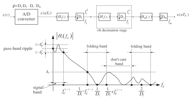
Figure 1: General architecture of a $m$-stage decimation chain for A/D converters, along with a pictorial representation of the key frequency intervals to be carefully considered for the design of the $i$th decimation stage. The sampling rate at the input of the $i$th decimation stage is $f_{i-1},~{}\forall i=1,\ldots,m$.

The design of multistage decimation filters for oversampled signals is a well-known research topic [1]. Mainly inspired by the need of computationally efficient architectures for wide-band, multi-standard, reconfigurable receiver design, this research topic has recently garnered new emphasis in the scientific community [2]-[5]. Multistage decimation filters are also employed for decimating highly oversampled signals from noise-shaping $\Sigma\Delta$ A/D converters [6].

Given a base-band analog input signal $x(t)$ with bandwidth $\left[-B_{x},+B_{x}\right]$, an A/D converter produces a digital signal $x(nT_{o})$ by sampling $x(t)$ at rate $f_{o}=\frac{1}{T_{o}}=2\rho B_{x}\gg 2B_{x}$, whereby $\rho\geq 1$ is the oversampling ratio (notice that $\rho>1$ for oversampled signals). The normalized maximum frequency contained in the input signal is defined as $f^{o}_{c}=\frac{B_{x}}{f_{o}}=\frac{1}{2\rho}$, and the digital signal $x(nT_{o})$ at the input of the first decimation filter has frequency components belonging to the range $[-f^{o}_{c},f^{o}_{c}]$. This setup is pictorially depicted in the reference architecture shown in Fig. 1.

Owing to the condition $\rho\gg 1$, the decimation of an oversampled signal $x(nT_{o})$ is efficiently [1] accomplished by cascading two (or more) decimation stages as highlighted in Fig. 1, in which a multistage architecture composed by $m$ decimation stages is shown as reference scheme. Consider an oversampling ratio $\rho$ which can be factorized as follows:

$$\rho=\prod_{i=1}^{m}D_{i}$$

whereby, for any $i$, $D_{i}$ is an appropriate integer strictly greater than zero.

In the general architecture shown in Fig. 1, sampling rate decreases in $m$ consecutive stages, whereby the sampling rate at the input of the $i$th stage is

$$f_{i-1}=f_{i}\cdot D_{i},~{}\forall i=1,\ldots,m$$

while the output sample data rate is:

$$f_{i}=\frac{f_{o}}{\prod_{p=1}^{i}D_{p}},~{}\forall i=1,\ldots,m$$

The design of any decimation stage in a multistage architecture imposes stringent constraints on the shape of the frequency response over the so-called folding bands. Considering the scheme in Fig. 1, the frequency response $H_{i}(e^{j\omega})$ of the $i$th decimation filter must attenuate the quantization noise (QN) falling inside the frequency ranges defined as

$$\begin{array}[]{lll}\left[\frac{k}{D_{i}}-f^{i-1}_{c};\frac{k}{D_{i}}+f^{i-1}_{c}\right],&k=1,...,k_{M}&\\ k_{M}=\lfloor\frac{D_{i}}{2}\rfloor,&D_{i}~{}\textrm{even}&\\ k_{M}=\lfloor\frac{D_{i}-1}{2}\rfloor,&D_{i}~{}\textrm{odd}&\end{array}$$ (1)

whereby $f^{i-1}_{c}$ is the normalized signal bandwidth at the input of the $i$th decimation filter. The reason is simple: the QN falling inside these frequency bands will fold down to baseband (i.e., inside the useful signal bandwidth $\left[-f^{i-1}_{c},+f^{i-1}_{c}\right]$) because of the sampling rate reduction by $D_{i}$ in the $i$th decimation stage, irremediably affecting the signal resolution after the multistage decimation chain.

On the other hand, frequency ranges labelled as don’t care bands in Fig. 1, do not require a stringent selectivity since the QN within these bands will be rejected by the subsequent filters in the multistage chain.

The relation between $f^{i}_{c}$ and $f^{o}_{c}$ is as follows:

$$f^{i}_{c}=f^{i-1}_{c}D_{i},~{}\forall i=1,\ldots,m$$

whereby it is $f^{o}_{c}=1/2\rho$.

The $i$th decimation filter $H_{i}(e^{j\omega})$ introduces a pass-band ripple $\delta^{i}_{p}$ which can also be expressed in dB as follows

$$R^{i}_{p}=-20\log_{10}\left(\frac{1-\delta^{i}_{p}}{1+\delta^{i}_{p}}\right)>0$$ (2)

while the selectivity (in dB) corresponds to

$$A_{s}=20\log_{10}\left(\frac{\delta_{s}}{1+\delta^{i}_{p}}\right)\approx 20\log_{10}\left(\delta_{s}\right)\ll 0$$ (3)

With this background, let us provide a quick survey of the recent literature related to the problem addressed here. This survey is by no means exhaustive and is meant to simply provide a sampling of the literature in this fertile area.

Excellent tutorials on the design of multirate filters can be found in [7, 8], while an essential book on this topic is [1]. Recently, Coffey [9, 10] addressed the design of optimized multistage decimation and interpolation filters.

The design of cascade-integrator comb (CIC) filters was first addressed in [11], while multirate architectures embedding comb filters have been discussed in [12]. Since then, many papers [13] have focused on the computational optimization of CIC filters even in the light of new wide-band and recofigurable receiver design applications [14]-[16]. Comb filters have been then generalized in [17]-[20], especially in relation to the decimation of $\Sigma\Delta$ modulated signals.

Other works somewhat related to the topic addressed in this paper are [21]-[27]. The use of decimation sharpened filters embedding comb filters is addressed in [20]-[21], while in [22] authors proposed computational efficient decimation filter architectures using polyphase decomposition of comb filters. Dolecek et al. proposed a novel two-stage sharpened comb decimator in [23]. The design of FIR filters using cyclotomic polynomial (CP) prefilters has been addressed in [24], while effective algorithms for the design of low-complexity FIR filters embedding CP prefilters have been proposed in [25]-[27].

Owing to the discussion on the folding bands presented above, this paper addresses the design of computationally efficient decimation filters suitable for oversampled digital signals. Natural eligible blocks used in filter design are cyclotomic polynomials with order less than $105$, since these polynomials possess coefficients belonging to the set $\{-1,0,+1\}$. We first recall the basic properties of CPs in Section II since these properties suggest useful hints at the basis of the practical implementation of the designed decimation filters. For conciseness, we address the design of the first stage in the multistage architecture, even though the considerations which follow are easily applicable to any other stage in the chain.

The computational complexity of basic CP filters is discussed in Section III. In Section IV we propose an optimization framework whose main aim is to design an optimal decimation filter (optimal in that the cost function to be minimized accounts for the number of additions required by the chosen CP filter) featuring high selectivity within the folding bands seen from the $i$th decimation stage.

The practical implementation of the designed decimation filters is addressed in Section V, whereby both recursive and non-recursive architectures stemming from a variety of properties of polynomials, are discussed. Finally, Section VI draws the conclusions.

II Basics of Cyclotomic Polynomials and Key Properties

Cyclotomic polynomials (CPs) arose hand in hand with the old Greek problem of dividing a circle in equal parts. Key properties of such polynomials along with the basic rationales can be found in various number theory books (we invite the interested readers to refer to [28, 29]), other than in some recent papers [24]. Given an integer $D$ strictly greater than zero, polynomial $\left(1-z^{-D}\right)$ can be factorized as a product of cyclotomic polynomials as follows:

TABLE I: Values of the totient function for $n\in[1,69]$. Symbol $\underline{1}$ is used to signify the fact that the underlined number is associated to $n=1$, while following numbers are associated to increasing values of $n$.

$\phi(n)$
1, 1, 2, 2, 4, 2, 6, 4, 6, 4, 10, 4, 12, 6, 8, 8, 16, 6, 18, 8, 12,
10, 22, 8, 20, 12, 18, 12, 28, 8, 30, 16, 20, 16, 24, 12, 36, 18,
24, 16, 40, 12, 42, 20, 24, 22, 46, 16, 42, 20, 32, 24, 52, 18,
40, 24, 36, 28, 58, 16, 60, 30, 36, 32, 48, 20, 66, 32, 44

$$1-z^{-D}=\prod_{q:q|D}^{D}C_{q}\left(z\right)$$ (4)

whereby $q:q|D$ identifies the set of integers $q$, less than, or equal to $D$, which divides $D$ (in other words, the remainder of the division between $D$ and $q$ is zero). For each $q$ as above, there is a unique polynomial $C_{q}\left(z\right)$ whose roots satisfy the following conditions.

• For each $q\leq D$, the roots of $C_{q}\left(z\right)$ constitute a subset of the roots belonging to the polynomial $1-z^{-D}$.

• The roots of $C_{q}\left(z\right)$ are the primitive $q$th roots of unity, i.e., they all fall on the $z$-plane unit circle.

• The number of roots corresponds to the number of positive integers which are prime with respect to $D$, and smaller than $D$.

• Roots of $C_{q}\left(z\right)$ do not belong to the set of roots of the polynomial $1-z^{-r},~{}\forall r:~{}0<r<q\leq D$.

Based on the observations above, polynomials $C_{q}\left(z\right)$ are defined as:

$$C_{q}\left(z\right)=\prod_{i:(i,q)=1}^{q}\left(1-z^{-1}e^{-j2\pi\frac{i}{q}}\right)$$ (5)

whereby $(i,q)=1$ is used to mean that $i$ and $q$ are co-prime [28]. Notice that, given an integer $q$, (5) allows us to write the $z$-transfer function of any CP indexed by $q$.

Key advantages of CPs in connection to filter design rely on the following property: if $q$ has no more than two distinct odd prime factors, polynomials $C_{q}\left(z\right)$ contains coefficients belonging to the set $\{-1,0,+1\}$. From a practical point of view, CP coefficients belong to the set $\{-1,0,+1\}$ if $q\leq 104$ [28, 29].

The degree of polynomial $C_{q}\left(z\right)$ is not $q$ but it is defined as follows:

$$\textrm{deg}\left[C_{q}\left(z\right)\right]=\sum_{d|q}d\cdot\mu\left(\frac{q}{d}\right)=\phi(q)$$ (6)

whereby $\phi(q)$ is the totient function (see Table I), i.e., the number of positive integers less or equal to $q$ that are relatively prime to $q$, while $\mu\left(n\right)$ is the M$\ddot{\textrm{o}}$bius function defined as:

$$\mu\left(n\right)=\left\{\begin{array}[]{ll}1,&n=1\\ (-1)^{k},&n=p_{1}\cdot p_{2}\cdot\ldots\cdot p_{k},\\ &\textrm{with}~{}p_{i}~{}\textrm{prime},~{}p_{i}\neq p_{j},~{}\forall i\neq j\\ 0,&\textrm{if n is divisible}\\ &\textrm{by the squares of a prime}\end{array}\right.$$ (7)

Index $k$ in the second entry stands for the number of distinct prime numbers which decomposes the argument $n$. Values of the M$\ddot{\textrm{o}}$bius function are shown in Table II for $n\in[1,104]$. Notice that $\mu\left(n\right)\neq 0$ implies that $n$ is squarefree, i.e., its decomposition does not contain repeated factors.

TABLE II: Values of the M$\ddot{\textrm{o}}$bius function for $n\in[1,104]$.

$\mu\left(n\right)$	$n$
$-1$	2, 3, 5, 7, 11, 13, 17, 19, 23, 29, 30, 31, 37, 41, 42,
	43, 47, 53, 59, 61, 66, 67, 70, 71, 73, 78, 79, 83, 89,
	97, 101, 102, 103
$1$	1, 6, 10, 14, 15, 21, 22, 26, 33, 34, 35, 38, 39, 46,
	51, 55, 57, 58, 62, 65, 69, 74, 77, 82, 85, 86, 87,
	91, 93, 94, 95
$0$	4, 8, 9, 12, 16, 18, 20, 24, 25, 27, 28, 32, 36, 40, 44,
	45, 48, 49, 50, 52, 54, 56, 60, 63, 64, 68, 72, 75, 76,
	80, 81, 84, 88, 90, 92, 96, 98, 99, 100, 104

The $z$-transfer function of a CP with squarefree index $q$ is [30]:

$$C_{q}(z)=\sum_{d=0}^{\phi(q)}c_{q,d}z^{-(\phi(q)-d)}$$ (8)

whereby coefficients $c_{q,d}$ can be evaluated with the following recursive relation:

$$c_{q,d}=-\frac{\mu(q)}{d}\sum_{p=0}^{d-1}c_{q,p}\cdot\mu\left(g(q,d-p)\right)\phi\left(g(q,d-p)\right)$$ (9)

using the initial value $c_{q,0}=1$. Function $g(q,d-p)$ in (9) is the greatest common divisor between $q$ and $d-p$. Notice that (9) represents an effective algorithm for automatically generating the $z$-transfer function of CPs with squarefree indexes $q$.

Perhaps, the main properties useful for deducing the $z$-transfer function of any CP, are the ones summarized in the following [28]. We will discuss the application of such properties in Section III whereby the focus is on the design of low complexity CPs in terms of both additions and delays.

1. Given a prime number $t$, it is

   $$C_{t}(z)=\sum_{i=0}^{t-1}z^{-i}=\frac{1-z^{-t}}{1-z^{-1}}$$ (10)

2. Let $k$, $n$ and $m$ be three positive integers. Then, it is

   $$C_{mn^{k}}\left(z\right)=C_{mn}\left(z^{n^{k-1}}\right)$$ (11)

3. Consider a prime number $p$, which does not divide $q$, then

   $$C_{pq}(z)=\frac{C_{q}(z^{p})}{C_{q}(z)}$$ (12)

4. Given any odd integer $n$ greater or equal to $3$, then it is

   $$C_{2n}(z)=C_{n}(-z)$$ (13)

5. For $z=1$, the following relation holds:

   $$C_{q}(1)=\left\{\begin{array}[]{ll}0,&q=1\\ p,&q=p^{k},~{}p~{}\textrm{prime}\\ 1,&\textrm{otherwise}\end{array}\right.$$ (14)

   This relation assures us that for indexes $q>1$, $z$-transfer function of the respective CP presents unity gain in baseband provided that $q\neq p^{k}$. Otherwise, CP transfer functions have to be normalized by $p$ in order to assure unity gain in baseband.

III Criteria for Identifying Low Complexity CPs

The $z$-transfer function of CPs for any index $q$ can be deduced upon employing the relation (5) along with the properties stated in (10)-(13). Different architectures (both recursive and non recursive) for implementing each CP can be obtained, mainly differing in the number of additions and delays required. For conciseness, in this paper we show the $z$-transfer functions of the first sixty CPs in Table IV; the $z$-transfer functions of $C_{q}(z)$ for any $q\in\{1,\ldots,104\}$ in both non recursive and recursive (if any) form can be found in [31].

Let us discuss some key examples by starting from CP $C_{33}(z)$. Considering that $33$ is squarefree and given that $p=33$ can be written as $3\times 11$, whereby $3$ and $11$ are coprimes, there are three possible architectures for implementing such a polynomial. The first one stems from (8) and (9) and it consists of a non recursive architecture (see Table IV) employing $14$ additions and $20$ delays. On the other hand, two recursive architectures follow upon using property (12) with $p=3,q=11$ and $p=11,q=3$:

$$\begin{array}[]{llll}C_{11\cdot 3}(z)&=\frac{C_{11}(z^{3})}{C_{11}(z)}&=\frac{1-z^{-33}}{1-z^{-3}}\cdot\frac{1-z^{-1}}{1-z^{-11}}&\\ &&=\frac{1-z^{-1}-z^{-33}+z^{-34}}{1-z^{-3}-z^{-11}+z^{-14}}&\\ C_{3\cdot 11}(z)&=\frac{C_{3}(z^{11})}{C_{3}(z)}&=\frac{1+z^{-11}+z^{-22}}{1+z^{-1}+z^{-2}}&\end{array}$$ (15)

As far as the number of additions is concerned, from (15) it easily follows that the architecture $C_{3\cdot 11}(z)$ only requires 4 additions, which compares favorably with both the non recursive implementation and $C_{11\cdot 3}(z)$. Notice also that, since CP coefficients are simply $\{-1,0,+1\}$, the recursive architectures can be implemented without coefficient quantization; this in turn suggests that exact pole-zero cancellation is not a concern with these architectures.

On the other hand, the non recursive architecture requires only $20$ delays as opposed to the recursive architectures requiring, respectively, $34$ and $22$ delays. In this work, we suppose that the computational complexity of the filter depends only on the number of additions.

Upon comparing for any $q$ both recursive and non recursive architectures in Table IV (see also the complete list of the first CPs reported in [31]), it easily follows that recursive implementations, when do exist, allow the reduction of the number of additions with respect to non recursive implementations; the price to pay, however, relies on the increased filter delay. As a rule of thumb, non recursive architectures should be preferred to recursive implementations when memory space is a design constraint. On the other hand, recursive architectures can greatly reduce the number of additions.

Let us briefly discuss the possible architectures related to an even indexed CP, such as $C_{60}(z)$. By virtue of the different ways to factorize the integer $60$, property (12) can be applied with the following combinations $p=5,q=12$, $p=3,q=20$ whereby in both cases $p$ is a prime integer not dividing $q$. Property (11) can be applied with $m=15,n=2,k=2$. In Table IV we show only both the recursive and the non recursive architectures yielding the lowest complexities.

When $q$ is a prime number, the $z$-transfer function of the related CP corresponds to the first order comb filter, as can be straightforwardly seen from (10). Finally, property (13) can be effectively employed for deducing the $z$-transfer function of CPs with even indexes $q$ which can be written as $2n$, with $n$ an odd number strictly greater than $2$. As an example, notice the following relations: $C_{30}(z)=C_{15}(-z)$, $C_{34}(z)=C_{17}(-z)$.

The simple examples presented above are by no means a complete picture of the capabilities and sophistication that can be found in multistage structures for sampling rate conversion. They are merely intended to show why such structures can constitute the starting point for obtaining computationally efficient filters for decimating oversampled signals. The design of computationally efficient decimation filters relies on the combination of an appropriate set of CPs. In oversampled A/D converters, for example, it is very important to contain the computational burden of the first stages in the multistage decimation chain. This motivates the study of an effective algorithm for identifying an appropriate set of CPs that, cascaded, is able to attain a set of prescribed requirements as specified in (2) and (3): this is the topic addressed in the next section.

IV Optimization Algorithm and Design Examples

TABLE III: Optimization results

$D=8$	Set of eligible CPs: $2,4,8,9,11,15,17,18,19,21,22,25,27,29,30,31,33,34,35,36,37,38,39,41,$
	$42,43,44,45,47,49,50,51,53,54,55,57,58,59,60,61,62,63,64$
$A_{s}=40,~{}R_{p}=1$dB	$H_{D8,1}(z)=C_{2}(z)C_{4}(z)C^{2}_{8}(z)C_{11}(z)$
$A_{s}=50,~{}R_{p}=1$dB	$H_{D8,2}(z)=C^{2}_{2}(z)C^{3}_{4}(z)C^{3}_{8}(z)$
$A_{s}=60,~{}R_{p}=1$dB	$H_{D8,3}(z)=C^{2}_{2}(z)C^{3}_{4}(z)C^{3}_{8}(z)C_{9}(z)$
$A_{s}=40,~{}R_{p}=2$dB	$H_{D8,4}(z)=C_{4}(z)C_{8}(z)C_{11}(z)C_{17}(z)$
$A_{s}=50,~{}R_{p}=2$dB	$H_{D8,5}(z)=C_{2}(z)C^{2}_{4}(z)C^{2}_{8}(z)C_{19}(z)$
$A_{s}=60,~{}R_{p}=2$dB	$H_{D8,6}(z)=C_{2}(z)C_{4}(z)C^{2}_{8}(z)C_{11}(z)C_{17}(z)$
$D=16$	Set of eligible CPs: $2,4,8,9,11,15,16,17,18,19,21,22,25,27,29,30,31,33,34,35,36,37,38,39,$
	$41,42,43,44,45,47,49,50,51,53,54,55,57,58,59,60,61,62,63,65,66,67,68,69,70,71,72,73,$
	$74,75,76,77,78,79,81,82,83,84,85,86,87,88,89,90,91,93,94,95,97,98,99,100,101,102,103$
$A_{s}=40,~{}R_{p}=1$dB	$H_{D16,1}(z)=C_{8}(z)C_{16}(z)C_{17}(z)C_{19}(z)$
$A_{s}=50,~{}R_{p}=1$dB	$H_{D16,2}(z)=C_{11}(z)C_{16}(z)C^{2}_{17}(z)$
$A_{s}=60,~{}R_{p}=1$dB	$H_{D16,3}(z)=C_{4}(z)C_{16}(z)C^{3}_{17}(z)$
$A_{s}=40,~{}R_{p}=2$dB	$H_{D16,4}(z)=C_{16}(z)C^{2}_{29}(z)$
$A_{s}=50,~{}R_{p}=2$dB	$H_{D16,5}(z)=C_{8}(z)C_{16}(z)C_{17}(z)C_{41}(z)$
$A_{s}=60,~{}R_{p}=2$dB	$H_{D16,6}(z)=C_{16}(z)C^{2}_{17}(z)C_{37}(z)$
$D=32$	Set of eligible CPs:$2,4,8,9,11,15,16,17,18,19,21,22,25,27,29,30,31,32,33,34,35,36,37,38,$
	$39,41,42,43,44,45,47,49,50,51,53,54,55,57,58,59,60,61,62,63,65,66,67,68,69,70,71,$
	$72,73,74,75,76,77,78,79,81,82,83,84,85,86,87,88,89,90,91,93,94,95,97,98,99,$
	$100,101,102,103$
$A_{s}=40,~{}R_{p}=1$dB	$H_{D32,1}(z)=C^{2}_{31}(z)C_{41}(z)$
$A_{s}=50,~{}R_{p}=1$dB	$H_{D32,2}(z)=C_{25}(z)C^{3}_{31}(z)$
$A_{s}=60,~{}R_{p}=1$dB	$H_{D32,3}(z)=C^{4}_{17}(z)$
$A_{s}=40,~{}R_{p}=2$dB	$H_{D32,4}(z)=C_{31}(z)C_{53}(z)C_{67}(z)$
$A_{s}=50,~{}R_{p}=2$dB	$H_{D32,5}(z)=C_{16}(z)C^{2}_{31}(z)C_{79}(z)$
$A_{s}=60,~{}R_{p}=2$dB	$H_{D32,6}(z)=C^{2}_{17}(z)C_{37}(z)C_{67}(z)$

This section presents an optimization framework for designing low complexity decimation filters, $H_{i}(z)$, as a cascade of CP subfilters. For the derivations which follow, consider the design of the $i$th decimation filter in the multistage chain depicted in Fig. 1, with a frequency response that can be represented as follows:

$$H_{i}\left(f_{d}\right)=\prod_{q=1}^{|S_{cp}|}C^{m_{q}}_{q}(f_{d})$$ (16)

whereby $f_{d}$ is the digital frequency normalized with respect to the sampling frequency $f_{i-1}$ as discussed in Section I, $S_{cp}$ is a suitable set of eligible CPs to be used in the optimization framework ($|S_{cp}|$ is the cardinality of the set, i.e., the number of eligible CPs), $C_{q}(f_{d})$ is the frequency response of the CP indexed by $q$ and $m_{q}$ is its integer order in the cascade constituting $H_{i}\left(f_{d}\right)$ (it is $m_{q}\geq 0,~{}\forall q$).

A suitable cost function accounting for the complexity of the $i$th decimation filter can be defined as a weighted combination of the number of adders and delays required by the overall filter $H_{i}(z)$ [26]:

$$F\left(m_{1},m_{2},\ldots,m_{|S_{cp}|}\right)=\sum_{q=1}^{|S_{cp}|}m_{q}\cdot\left(N_{a,q}+\gamma\cdot N_{d,q}\right)$$ (17)

whereby $N_{a,q}$ and $N_{d,q}$ are, respectively, the number of adders and delays of CP $C_{q}(z)$, and $\gamma\in[0,1]$ is a factor depending on the relative complexity of the delays with respect to the adders. In our setup, we assume that the computational complexity of the $i$th decimation filter is mainly due to the number of adders; therefore, we set $\gamma=0$. Notice that the cost function depends on the CP orders $m_{1},\ldots,m_{|S_{cp}|}$, while $N_{a,q}$ and $N_{d,q}$ are known once the set $S_{cp}$ of eligible CPs has been appropriately identified. Notice also that $N_{a,q}$ and $N_{d,q}$ can be straightforwardly obtained by Table IV (see also [31] for a list of all 104 CPs).

Let us address the choice of the eligible CPs in the set $S_{cp}$. This is one of the most important design step since the complexity of the optimization framework discussed below, is tied tightly to the number of eligible CPs. By virtue of the discussion on the folding bands spanned by the $i$th decimation filter, we choose the eligible CPs between the $104$ CPs in such a way that 1) at least 20% of zeros falls within the folding bands defined in (1), 2) no zero falls in the signal pass-band ranging from $0$ to $f^{o}_{c}$. As a result of extensive tests, we adopted such a threshold which is capable to reject about $20-60$ initial CPs depending on $D$. Of course, lower thresholds can increase the number of eligible CPs at the cost of an increased complexity of the optimization framework discussed below. On the other hand, when designing the $i$th decimation filter in a multistage architecture, only the so-called folding bands must be spanned by zeros, since don’t care frequency bands will be appropriately spanned by the zeros belonging to the subsequent decimation filters in the cascade.

Before presenting the optimization algorithm, let us discuss the requirements imposed to the frequency response $H_{i}(f_{d})$ of the $i$th decimation filter in the cascade. Mask specifications [1] are given as for classical filters as far as the passband ripple is concerned. In particular, for the optimization algorithm we use the passband ripple expressed in dB as specified in (2). The main difference between the design proposed in this work and classical FIR filter design techniques relies on the fact that in our setup specifications are only imposed in the folding bands (1). To this end, we evaluated the lowest attenuations (worst-case) attained by each CP belonging to $S_{cp}$ in each folding band:

$$\begin{array}[]{ll}A_{d_{q}}=-\max_{f_{d}\in\left[0;+f^{i-1}_{c}\right]}20\log_{10}\left(|C_{q}(f_{d})|_{n}\right)&\\ &\\ A_{s}(k,q)=\min_{f_{d}\in\left[\frac{k}{D_{i}}-f^{i-1}_{c};\frac{k}{D_{i}}+f^{i-1}_{c}\right]}20\log_{10}\left(|C_{q}(f_{d})|_{n}\right)&\end{array}$$ (18)

whereby subscript $n$ signifies the fact that each CP $C_{q}$ has been normalized in such a way as to have unity gain in baseband. Notice that normalization factors can be deduced from (14). $A_{s}(k,q)$ is the worst attenuation of the $q$th CP in $S_{cp}$ within the $k$th folding band, with $k\in\{1,\ldots,k_{M}\}$, and $k_{M}$ defined in (1). Such values (in dB) have been stored in look-up tables.

Once the set $S_{cp}$ of eligible CPs along with the appropriate specifications (passband ripple and folding band attenuations) have been identified, the optimization problem can be formulated as follows:

$$\begin{array}[]{lll}\min_{m_{1},\ldots,m_{|S_{cp}|}}F\left(m_{1},\ldots,m_{|S_{cp}|}\right)\left|{}_{\gamma=0}\right.~{}\textrm{in}~{}(\ref{power_consumption})&&\\ \textrm{subject~{}to:}&&\\ \begin{array}[]{llll}0)&\sum_{q=1}^{|S_{cp}|}m_{q}A_{d_{q}}&\leq&R_{p}~{}\textrm{(ripple)}\\ 1)&\sum_{q=1}^{|S_{cp}|}m_{q}A_{s}(1,q)&\leq&A_{s}~{}\textrm{(selectivity)}\\ &\ldots&\ldots&\\ k)&\sum_{q=1}^{|S_{cp}|}m_{q}A_{s}(k,q)&\leq&A_{s}\\ &\ldots&\ldots&\\ k_{M})&\sum_{q=1}^{|S_{cp}|}m_{q}A_{s}(k_{M},q)&\leq&A_{s}\\ \end{array}\end{array}$$ (19)

The optimization problem can be also solved for different prescribed selectivities, $A_{s}$ (as specified in (3)), around the various folding bands. In this work we do not pursue this approach. However, notice that such an approach can be effective for noise shaping $\Sigma\Delta$ A/D converters which present an increasing noise power spectra density for higher and higher values of the digital frequency $f_{d}<1/2$ [6, 18]. Setting increasing values of $|A_{s}|$ in correspondence of successive folding bands can mitigate noise folding due to the decimation process.

The solution to the optimization problem (19) is the set of CP orders $\textbf{m}=[m_{1},\ldots,m_{|S_{cp}|}]^{T}$, whereby $m_{i}=0$ signifies the fact that the $i$th CP in $S_{cp}$ is not employed for synthesizing $H_{i}(f_{d})$.

Upon collecting the set of $k_{M}+1$ conditions in the matrix A:

$$\textbf{A}=\left(\begin{array}[]{ccccc}A_{d_{1}}&\ldots&A_{d_{|S_{cp}|}}\\ A_{s}(1,1)&\ldots&A_{s}(1,|S_{cp}|)\\ \ldots&\ldots&\ldots\\ A_{s}(k_{M},1)&\ldots&A_{s}(k_{M},|S_{cp}|)\\ \end{array}\right)$$

and the requirements $\textbf{b}=[R_{p}~{}A_{s}~{}\ldots~{}A_{s}]^{T}$, the constraints in (19) can be rewritten as follows:

$$\textbf{A}\textbf{m}\leq\textbf{b}$$

By this setup, the optimization problem in (19) with respect to $m_{1},\ldots,m_{|C^{S}_{p}|}$ can be rewritten as

$$\begin{array}[]{lll}\min_{m_{1},\ldots,m_{|S_{cp}|}}F\left(m_{1},\ldots,m_{|S_{cp}|}\right)\left|{}_{\gamma=0}\right.&&\\ \textrm{subject~{}to:}&&\\ \begin{array}[]{lll}&\textbf{A}\textbf{m}\leq\textbf{b}&\\ &m_{i}\geq 0,~{}m_{i}~{}\textrm{integer},&\forall i=1,\ldots,|S_{cp}|\\ \end{array}\end{array}$$

and solved by mixed integer linear programming techniques [32]. We solved the optimization problem using the Matlab function linprog along with a new matlab file capable of managing integer constrained solutions (the latter file is available online [33]).

The results of the previous optimization problem are summarized in Table III for various $A_{s}$ specifications and two different values of $R_{p}$, namely $R_{p}=1$ and $2$ dB. We solved the problem for three different values of the decimation factor $D$ of the first stage in the decimation chain depicted in Fig. 1 by assuming that the residual decimation factor is $\nu=4$ (in other words, we assumed that $\rho=D\cdot 4$). Notice that such an approach is quite usual in practice in that the first decimation filter accomplishes the highest possible decimation in order to reduce the sampling rate, while the subsequent decimation stages are usually accomplished with half-band filters each one decimating by $2$ [1].

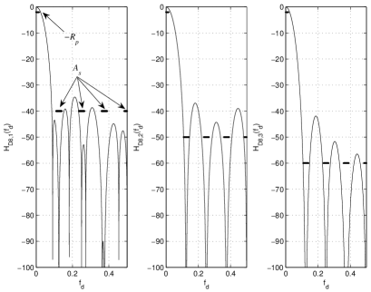
Figure 2: Behaviours in dB of the modulo of the frequency responses $H_{8,1}(f_{d}),H_{8,2}(f_{d}),H_{8,3}(f_{d})$ of the optimized decimation filters shown in Table III for $D=8$.

The first row related to any decimation factor shows the set of eligible CPs found in the preliminary design step discussed above, while the $z$-transfer functions of the CPs can be found in Table IV (see also [31] for a list of all 104 CPs).

It is worth comparing the frequency responses of the optimized filters $H_{8,i}(f_{d})$ and $H_{16,i}(f_{d})$ (for $i=1,2,3$) in Table III with the specifications $R_{p}=1$dB and various $A_{s}$. To this end, Fig.s 2 and 3 show, respectively, the behaviours of the frequency responses $H_{8,i}(f_{d})$ and $H_{16,i}(f_{d})$ along with the imposed selectivity $A_{s}$ around the various folding bands (identified by horizontal bold lines).

V Implementation Issues

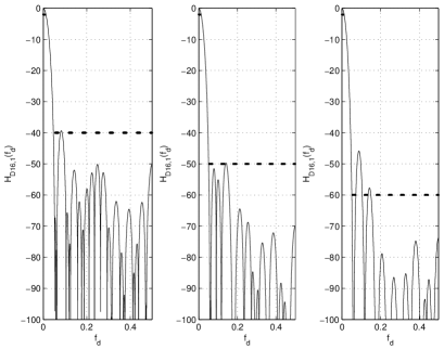
Figure 3: Behaviours in dB of the modulo of the frequency responses $H_{16,1}(f_{d}),H_{16,2}(f_{d}),H_{16,3}(f_{d})$ of the optimized decimation filters shown in Table III for $D=16$.

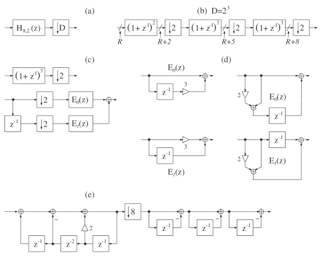
Figure 4: Efficient architectures for implementing the decimation stage embedding $H_{8,2}(z)$ (a). Non recursive architecture (b); polyphase implementation of the decimation stages decimating by $2$ (c), and polyphase component implementation using shift registers (d); recursive architecture of the decimation filter $H_{8,2}(z)$ (e).

This section addresses the design of optimized CP-based decimation filters. For conciseness, we will focus on the design of decimation filter $H_{8,2}(z)$ shown in Table III, even though the considerations which follow can be applied to any other decimation filter quite straightforwardly. The decimation stage related to $H_{8,2}(z)$ is depicted in Fig. 4a: this decimation filter will be designed through a variety of architectures following from different mathematical ways to simplifies the analytical relation defining $H_{8,2}(z)$.

First of all, notice that upon substituting the appropriate equations of the constituent CP filters in $H_{8,2}(z)$, the designed filter takes on the following expression:

$$H_{8,2}(z) = C_{2}^{2}(z)C_{4}^{3}(z)C_{8}^{3}(z)=$$

$$= \left(1+z^{-1}\right)^{2}\left(1+z^{-2}\right)^{3}\left(1+z^{-4}\right)^{3}$$

which can be rewritten as follows:

$$H_{8,2}(z) = \frac{\prod_{i=0}^{2}\left(1+z^{-2^{i}}\right)^{3}}{1+z^{-1}}$$ (21)

From the commutative property employed in [12], the cascaded implementation shown in Fig. 4b easily follows. The $r$th stage in Fig. 4b operates at the sampling rate $f_{i-1}/2^{r}$, whereby $f_{i-1}$ is the data sampling frequency at the filter input as shown in the multistage architecture in Fig. 1. Further power consumption reduction can be achieved by applying polyphase decomposition to the architecture shown in Fig. 4b. To this aim, consider the $z$-transfer function of the $3$rd order cell:

$$\left(1+z^{-1}\right)^{3} = 1+3z^{-2}+z^{-1}\left(3+z^{-2}\right)$$

$$= E_{0}(z^{2})+z^{-1}E_{1}(z^{2})$$

$$E_{0}(z) = 1+3z^{-1}$$

$$E_{1}(z) = 3+z^{-1}$$ (22)

The polyphase architecture for $\left(1+z^{-1}\right)^{3}$ easily follows from the commutative property applied to the two filters $E_{0}(z^{2})$ and $E_{1}(z^{2})$ in (V), and it is shown in Fig. 4c along with the architectures for implementing both $E_{0}(z)$ and $E_{1}(z)$. Notice that the multipliers appearing in $E_{0}(z)$ and $E_{1}(z)$ can be implemented in the form of shift registers as depicted in Fig. 4d.

The actual complexity of the architecture shown in Fig. 4b is fully defined once the data wordlength in any substage is well characterized, since the power consumption of a filter cell can be approximated as the product between the data rate, the number of additions performed at that rate, and the data wordlength. While the data rate along with the number of additions are well defined, data wordlength in each substage in Fig. 4b is not. Given the input data wordlength, $R$ (in bits), the data size at the output of the first decimation substage in Fig. 4b is equal to $R+2$ bits since two carry bits have to be allocated for the two additions involved in that substage. With a similar reasoning, data wordlength increases at the output of each subsequent substage in Fig. 4b in order to take into account the increase of data size due to the involved additions.

As a reference example, if the decimation filter depicted in Fig. 4b is the first decimation stage at the output of a $\Sigma\Delta$ A/D converter embedding a $1$-bit quantizer into the loop, it is $R=1$. Thus, data wordlength is as low as $3$ bits after the first decimation substage, and so on.

Let us address the design of a recursive architecture for $H_{8,2}(z)$ in (V). First of all, consider the following equality chain

$$\prod_{i=0}^{\log_{2}(D)-1}\left(1+z^{-2^{i}}\right)^{t}=\left[\sum_{i=0}^{D-1}z^{-i}\right]^{t}=\left[\frac{1-z^{-D}}{1-z^{-1}}\right]^{t}$$ (23)

whereby the first equality holds for any $D$ that can be written as an integer power of $2$, i.e., $D=2^{p}$. On the other hand, the last equality holds for any integer value of $D$. Notice that decimation factors of the form $2^{p}$ are quite common in practice. Upon using (23) with $t=3$ and $D=2^{3}$, (V) can be rewritten as follows:

$$\begin{array}[]{lll}H_{8,2}(z)&=&\left[\prod_{i=0}^{2}\left(1+z^{-2^{i}}\right)^{3}\right]\frac{1}{1+z^{-1}}\\ &=&\left[\frac{1-z^{-8}}{1-z^{-1}}\right]^{3}\frac{1}{1+z^{-1}}\end{array}$$

The last relation in (V) can be simplified as follows:

$$\small\frac{(1-z^{-8})^{3}}{(1-z^{-1})^{3}(1+z^{-1})}=\frac{(1-z^{-8})^{3}}{1-2z^{-1}+2z^{-3}-z^{-4}}$$ (24)

A recursive implementation of filter $H_{8,2}(z)$ in (24) is shown in Fig. 4e. It is obtained in the same way as for a classic cascade integrator-comb (CIC) implementation [11]. In other words, the numerator in (24) corresponds to the comb sections at the right of the decimator by $D$, while the denominator is responsible for the integrator sections at the left of the decimator by $D=8$.

The derivations yielding (24) upon starting from (V) can also be accomplished by following another reasoning based on the following relation:

$$1+z^{-n}=\frac{1-z^{-2n}}{1-z^{-n}}$$ (25)

which is valid for any positive $n=2^{t-1}w$ with $w$ an odd integer. By doing so, (V) can be rewritten as follows:

$$H_{8,2}(z) = \left(1+z^{-1}\right)^{2}\left(1+z^{-2}\right)^{3}\left(1+z^{-4}\right)^{3}$$

$$= \left(\frac{1-z^{-2}}{1-z^{-1}}\right)^{2}\left(\frac{1-z^{-4}}{1-z^{-2}}\right)^{3}\left(\frac{1-z^{-8}}{1-z^{-4}}\right)^{3}$$

Upon simplifying, (V) yields (24).

An alternative non recursive architecture stems from a full polyphase decomposition of the transfer function $H_{8,2}(z)$. Upon solving polynomial multiplications in (V), $H_{8,2}(z)$ can be rewritten as follows:

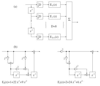
Figure 5: Architecture of the polyphase implementation of the decimation filter $H_{8,2}(z)$ (a), and efficient design of the first two polyphase components $E_{0}(z)$ and $E_{1}(z)$ (b).

$$H_{8,2}(z)=\sum_{i=0}^{20}h(i)z^{-i}$$ (27)

By applying the polyphase decomposition [34], $H_{8,2}(z)$ can be rewritten as

$$H(z) = \sum_{i=0}^{D-1}z^{-i}E_{i}(z^{D})$$ (28)

$$E_{i}(z) = \sum_{t=0}^{\left\lfloor\frac{L}{D}\right\rfloor}h(D\cdot t+i)z^{-t},~{}0\leq i\leq D-1$$

whereby $L=21$ is the length of the impulse response. The $z$-transfer function in (28) is implemented with the architecture shown in Fig. 5a. The polyphase components $E_{i}(z),~{}0\leq i\leq D-1=7,$ can be easily obtained by employing (27). In particular, the first two polyphase components take on the following expressions:

$$\begin{array}[]{lll}E_{0}(z)&=&1+22z^{-1}+9z^{-2}\\ &=&(2^{3}+2^{0})z^{-1}(2+z^{-1})+2^{2}z^{-1}+1\\ E_{1}(z)&=&2+24z^{-1}+6z^{-2}\\ &=&2\left[1+(2^{1}+1)z^{-1}(z^{-1}+2^{2})\right]\end{array}$$ (29)

An efficient architecture for implementing each polyphase component $E_{i}(z)$ stems from the decomposition of each integer as the summation of power-of-two coefficients as shown in (29) for the first two polyphase components $E_{0}(z)$ and $E_{1}(z)$. By doing so, and employing coefficient sharing arguments, practical architectures featuring a minimum number of shift registers easily follow as depicted in Fig. 5b. Similar considerations can be employed for obtaining the architectures of the remaining polyphase components $E_{2}(z),\ldots,E_{7}(z)$.

VI Conclusions

This paper addressed the design of multiplier-less decimation filters suitable for oversampled digital signals. The aim was twofold. On one hand, it proposed an optimization framework for the design of constituent decimation filters in a general multistage decimation architecture using as basic building blocks cyclotomic polynomials (CPs), since the first 104 CPs have simple coefficients ($\{-1,0,+1\}$). On the other hand, the paper provided a bunch of useful techniques, most of which stemming from some key properties of CPs, for designing the optimized filters in a variety of architectures. Both recursive and non-recursive architectures have been discussed by focusing on a specific decimation filter obtained as a result of the optimization algorithm. Design guidelines were provided with the aim to simplify the design of the constituent decimation filters in the multistage chain.

TABLE IV: The first sixty cyclotomic polynomials.

$q$	$C_{q}(z^{-1})$	$q$	$C_{q}(z^{-1})$	$q$	$C_{q}(z^{-1})$
1	$1-z^{-1}$	11	$\sum_{i=0}^{10}z^{-i}=\frac{1-z^{-11}}{1-z^{-1}}$	21	$1-z^{-1}+z^{-3}-z^{-4}+z^{-6}$
					$-z^{-8}+z^{-9}-z^{-11}+z^{-12}$
					$=\frac{1+z^{-7}+z^{-14}}{1+z^{-1}+z^{-2}}$
2	$1+z^{-1}$	12	$1-z^{-2}+z^{-4}=\frac{1+z^{-6}}{1+z^{-2}}$	22	$\sum_{i=0}^{10}(-1)^{i}z^{-i}=\frac{1+z^{-11}}{1+z^{-1}}$
3	$1+z^{-1}+z^{-2}=\frac{1-z^{-3}}{1-z^{-1}}$	13	$\sum_{i=0}^{12}z^{-i}=\frac{1-z^{-13}}{1-z^{-1}}$	23	$\frac{1-z^{-23}}{1-z^{-1}}$
4	$1+z^{-2}$	14	$\sum_{i=0}^{6}(-1)^{i}z^{-i}=\frac{1+z^{-7}}{1+z^{-1}}$	24	$1-z^{-4}+z^{-8}=\frac{1+z^{-12}}{1+z^{-4}}$
5	$\frac{1-z^{-5}}{1-z^{-1}}$	15	$1-z^{-1}+z^{-3}-z^{-4}+z^{-5}$	25	$\sum_{i=0}^{4}z^{-5i}=\frac{1-z^{-25}}{1-z^{-5}}$
			$-z^{-7}+z^{-8}=\frac{1+z^{-5}+z^{-10}}{1+z^{-1}+z^{-2}}$
6	$1-z^{-1}+z^{-2}=\frac{1+z^{-3}}{1+z^{-1}}$	16	$1+z^{-8}$	26	$\sum_{i=0}^{12}(-1)^{i}z^{-i}=\frac{1+z^{-13}}{1+z^{-1}}$
7	$\frac{1-z^{-7}}{1-z^{-1}}$	17	$\sum_{i=0}^{16}z^{-i}=\frac{1-z^{-17}}{1-z^{-1}}$	27	$1+z^{-9}+z^{-18}=\frac{1-z^{-27}}{1-z^{-9}}$
8	$1+z^{-4}$	18	$1-z^{-3}+z^{-6}=\frac{1+z^{-9}}{1+z^{-3}}$	28	$\sum_{i=0}^{6}(-1)^{i}z^{-2i}=\frac{1+z^{-14}}{1+z^{-2}}$
9	$1+z^{-3}+z^{-6}=\frac{1-z^{-9}}{1-z^{-3}}$	19	$\sum_{i=0}^{18}z^{-i}=\frac{1-z^{-19}}{1-z^{-1}}$	29	$\frac{1-z^{-29}}{1-z^{-1}}$
10	$\sum_{i=0}^{4}(-1)^{i}z^{-i}=\frac{1+z^{-5}}{1+z^{-1}}$	20	$1-z^{-2}+z^{-4}-z^{-6}+z^{-8}$	30	$1+z^{-1}-z^{-3}-z^{-4}-z^{-5}$
			$=\frac{1+z^{-10}}{1+z^{-2}}$		$+z^{-7}+z^{-8}=\frac{1-z^{-5}+z^{-10}}{1-z^{-1}+z^{-2}}$
31	$\frac{1-z^{-31}}{1-z^{-1}}$	41	$\frac{1-z^{-41}}{1-z^{-1}}$	51	$1-z^{-1}+z^{-3}-z^{-4}+z^{-6}-z^{-7}$
					$z^{-9}-z^{-10}+z^{-12}-z^{-13}+z^{-15}$
					$-z^{-16}+z^{-17}-z^{-19}+z^{-20}-z^{-22}$
					$z^{-23}-z^{-25}+z^{-26}-z^{-28}+z^{-29}$
					$-z^{-31}+z^{-32}=\frac{1-z^{-51}}{1-z^{-3}}\cdot\frac{1-z^{-1}}{1-z^{-17}}$
32	$1+z^{-16}$	42	$1+z^{-1}-z^{-3}-z^{-4}+z^{-6}$	52	$\sum_{i=0}^{12}(-1)^{i}z^{-2i}=\frac{1+z^{-26}}{1+z^{-2}}$
			$-z^{-8}-z^{-9}+z^{-11}+z^{-12}$
			$=\frac{1-z^{-7}+z^{-14}}{1-z^{-1}+z^{-2}}$
33	$1-z^{-1}+z^{-3}-z^{-4}+z^{-6}$	43	$\frac{1-z^{-43}}{1-z^{-1}}$	53	$\frac{1-z^{-53}}{1-z^{-1}}$
	$-z^{-7}+z^{-9}-z^{-10}+z^{-11}$
	$-z^{-13}+z^{-14}-z^{-16}+z^{-17}$
	$-z^{-19}+z^{-20}=\frac{1+z^{-11}+z^{-22}}{1+z^{-1}+z^{-2}}$
34	$\sum_{i=0}^{16}(-1)^{i}z^{-i}=\frac{1+z^{-17}}{1+z^{-1}}$	44	$\sum_{i=0}^{10}(-1)^{i}z^{-2i}=\frac{1+z^{-22}}{1+z^{-2}}$	54	$1-z^{-9}+z^{-18}$
35	$1-z^{-1}+z^{-5}-z^{-6}+z^{-7}$	45	$1-z^{-3}+z^{-9}-z^{-12}$	55	$1-z^{-1}+z^{-5}-z^{-6}+z^{-10}-z^{-12}$
	$-z^{-8}+z^{-10}-z^{-11}+z^{-12}$		$+z^{-15}-z^{-21}+z^{-24}$		$z^{-15}-z^{-17}+z^{-20}-z^{-23}+z^{-25}$
	$-z^{-13}+z^{-14}-z^{-16}+z^{-17}$		$=\frac{1+z^{-15}+z^{-30}}{1+z^{-3}+z^{-6}}$		$-z^{-28}+z^{-30}-z^{-34}+z^{-35}$
	$-z^{-18}+z^{-19}-z^{-23}+z^{-24}$				$-z^{-39}+z^{-40}=\frac{1-z^{-55}}{1-z^{-5}}\cdot\frac{1-z^{-1}}{1-z^{-11}}$
	$=\frac{1-z^{-1}-z^{-35}+z^{-36}}{1-z^{-5}-z^{-7}+z^{-12}}$
36	$1-z^{-6}+z^{-12}$	46	$\sum_{i=0}^{22}(-1)^{i}z^{-i}=\frac{1+z^{-23}}{1+z^{-1}}$	56	$\sum_{i=0}^{6}(-1)^{i}z^{-4i}=\frac{1+z^{-28}}{1+z^{-4}}$
37	$\frac{1-z^{-37}}{1-z^{-1}}$	47	$\frac{1-z^{-47}}{1-z^{-1}}$	57	$1-z^{-1}+z^{-3}-z^{-4}+z^{-6}-z^{-7}$
					$+z^{-9}-z^{-10}+z^{-12}-z^{-13}$
					$+z^{-15}-z^{-16}+z^{-18}-z^{-20}+z^{-21}$
					$-z^{-23}+z^{-24}-z^{-26}+z^{-27}-z^{-29}$
					$+z^{-30}-z^{-32}+z^{-33}-z^{-35}+z^{-36}$
					$=\frac{1-z^{-57}}{1-z^{-3}}\cdot\frac{1-z^{-1}}{1-z^{-19}}$
38	$\sum_{i=0}^{18}(-1)^{i}z^{-i}=\frac{1+z^{-19}}{1+z^{-1}}$	48	$1-z^{-8}+z^{-16}$	58	$\sum_{i=0}^{28}(-1)^{i}z^{-i}=\frac{1+z^{-29}}{1+z^{-1}}$
39	$1-z^{-1}+z^{-3}-z^{-4}+z^{-6}$	49	$\sum_{i=0}^{6}z^{-7i}=\frac{1-z^{-49}}{1-z^{-7}}$	59	$\frac{1-z^{-59}}{1-z^{-1}}$
	$-z^{-7}+z^{-9}-z^{-10}+z^{-12}$
	$-z^{-14}+z^{-15}-z^{-17}+z^{-18}$
	$-z^{-20}+z^{-21}-z^{-23}+z^{-24}$
	$=\frac{1-z^{-39}}{1-z^{-3}}\cdot\frac{1-z^{-1}}{1-z^{-13}}$
40	$\sum_{i=0}^{4}(-1)^{i}z^{-4i}=\frac{1+z^{-20}}{1+z^{-4}}$	50	$\sum_{i=0}^{4}(-1)^{i}z^{-5i}=\frac{1+z^{-25}}{1+z^{-5}}$	60	$1+z^{-2}-z^{-6}-z^{-8}-z^{-10}$
					$+z^{-14}+z^{-16}=\frac{1-z^{-10}+z^{-20}}{1-z^{-2}+z^{-4}}$

References

- [1] R. E. Crochiere and L. R. Rabiner, Multirate Digital Signal Processing, Prentice-Hall PTR, 1983.
- [2] J. Mitola, “The software radio architecture,” IEEE Comm. Magazine, Vol.33, No.5, pp. 26-38, May 1995.
- [3] M. Laddomada, F. Daneshgaran, M. Mondin, and R.M. Hickling, “A PC-based software receiver using a novel front-end technology,” IEEE Comm. Magazine, Vol.39, No.8, pp.136-145, Aug. 2001.
- [4] F. Daneshgaran and M. Laddomada, “Transceiver front-end technology for software radio implementation of wideband satellite communication systems,” Wireless Personal Communications, Kluwer, Vol.24, No.12, pp. 99-121, December 2002.
- [5] A.A. Abidi, “The path to the software-defined radio receiver,” IEEE Journal of Solid-State Circuits, Vol.42, No.5, pp. 954-966, May 2007.
- [6] S. R. Norsworthy, R. Schreier, and G. C. Temes, Delta-Sigma Data Converters, Theory, Design, and Simulation, IEEE Press, 1997.
- [7] R. E. Crochiere and L. R. Rabiner, “Interpolation and decimation of digital signals A tutorial review,” Proceedings of the IEEE, Vol.69, No.3, pp. 300-331, March 1981.
- [8] P.P. Vaidyanathan, “Multirate digital filters, filter banks, polyphase networks, and applications: a tutorial,” Proceedings of the IEEE, Vol.78, No.1, pp. 56-93, Jan. 1990.
- [9] M.W. Coffey, “Optimizing multistage decimation and interpolation processing-Part I,” IEEE Signal Proc. Letters, Vol.10, No.4, pp. 107-110, April 2003.
- [10] M.W. Coffey, “Optimizing multistage decimation and interpolation processing-Part II,” IEEE Signal Proc. Letters, Vol.14, No.1, pp. 24-26, Jan. 2007.
- [11] E. B. Hogenauer, “An economical class of digital filters for decimation and interpolation,” IEEE Trans. on Ac., Speech and Sign. Proc., Vol. ASSP-29, pp. 155-162, No. 2, April 1981.
- [12] S. Chu and C. S. Burrus, “Multirate filter designs using comb filters,” IEEE Trans. on Circuits and Systems, vol. CAS-31, pp. 913 924, Nov. 1984.
- [13] R.A. Losada and R. Lyons, “Reducing CIC filter complexity,” IEEE Signal Proc. Mag., Vol.23, No.4, pp. 124-126, July 2006.
- [14] Y. Gao, J. Tenhunen, and H. Tenhunen, “A fifth-order comb decimation filter for multi-standard transceiver applications,” In Proceedings of ISCAS 2000, May 28-31, 2000, Geneva, Switzerland, pp. III-89-III-92.
- [15] F.J.A. de Aquino, C.A.F. da Rocha, and L.S. Resende, “Design of CIC filters for software radio system,” Proceedings of IEEE ICASSP 2006, Vol.3, 2006.
- [16] T. Ze and S. Signell, “Multi-standard delta-sigma decimation filter design,” Proceedings of IEEE APCCAS 2006, pp. 1212-1215, 4-7 Dec. 2006.
- [17] L. Lo Presti, “Efficient modified-sinc filters for sigma-delta A/D converters,” IEEE Trans. on Circ. and Syst.-II, Vol. 47, pp. 1204-1213, No. 11, November 2000.
- [18] M. Laddomada, “Generalized comb decimation filters for A/D converters: Analysis and design,” IEEE Trans. on Circuits and Systems I, Vol.54, No. 5, pp. 994-1005, May 2007.
- [19] M. Laddomada and M. Mondin, “Decimation schemes for A/D converters based on Kaiser and Hamming sharpened filters,” IEE Proceedings of Vision, Image and Signal Processing, Vol. 151, No. 4, pp. 287-296, August 2004.
- [20] M. Laddomada, “Comb-based decimation filters for A/D converters: Novel schemes and comparisons,” IEEE Trans. on Signal Processing, Vol.55, No. 5, Part 1, pp. 1769-1779, May 2007.
- [21] A.Y. Kwentus, Z. Jiang, and A.N. Willson Jr., “Application of filter sharpening to cascaded integrator-comb decimation filters,” IEEE Trans. on Signal Proc., Vol. 45, pp. 457-467, No. 2, February 1997.
- [22] H. Aboushady, Y. Dumonteix, M. Lourat, and H. Mehrez, “Efficient polyphase decomposition of comb decimation filters in analog-to-digital converters,” IEEE Trans. on Circ. and Syst.-II, Vol. 48, pp. 898-903, No. 10, October 2001.
- [23] G. Jovanovic-Dolecek and S.K. Mitra, “A new two-stage sharpened comb decimator,” IEEE Trans. on Circ. and Syst.-I, Vol. 52, pp. 1414-1420, No. 7, July 2005.
- [24] R.J. Hartnett and G.F. Boudreaux-Bartels, “On the use of cyclotomic polynomial prefilters for efficient FIR filter design,” IEEE Trans. on Signal Processing, Vol.41, No.5, pp. 1766-1779, May 1993.
- [25] H.J. Oh and Y.H. Lee, “Design of efficient FIR filters with cyclotomic polynomial prefilters using mixed integer linear programming,” IEEE Signal Proc. Letters, Vol.3, No.8, pp. 239-241, Aug. 1996.
- [26] H.J. Oh and Y.H. Lee, “Design of discrete coefficient FIR and IIR digital filters with prefilter-equalizer structure using linear programming,” IEEE Trans. on Circuits and Systems II, Vol.47, No.6, pp. 562-565, June 2000.
- [27] K. Supramaniam and Yong Lian, “Complexity reduction for frequency-response masking filters using cyclotomic polynomial prefilters,” Proceedings of IEEE ISCAS 2006, 21-24 May 2006.
- [28] M.R. Schroeder, Number Theory in Science and Communication: With Applications in Cryptography, Physics, Digital Information, Computing, and Self-Similarity, Springer-Verlag, 3rd ed., 1997.
- [29] J.H. McClellan and C.M. Rader, Number Theory in Digital Signal Processing, Prentice-Hall, 1979.
-
[30]
http://mathworld.wolfram.com/CyclotomicPolynomial.html -
[31]
M. Laddomada,
“Some Properties along with the -transfer functions of the
first 104 Cyclotomic Polynomials,” Internal report,
available at
http://www.tlc.polito.it/dcc_team/research.php?id=4 - [32] C.H. Papadimitriou and K. Steiglitz, Combinatorial Optimizaion, Algorithms and Complexity, Dover Publications, Mineola, New York, 1998.
-
[33]
Mixed Integer Linear Programming Matlab file, available at
http://www.mathworks.com/matlabcentral/fileexchange/loadFile.do?objectId=6990&objectType=file - [34] A. Antoniou, Digital Signal Processing: Signals, Systems, and Filters, McGraw-Hill, 2005, ISBN 0-07-145425-X.