Strain distribution in quantum dot of arbitrary polyhedral shape:
Analytical solution in closed form

Abstract

An analytical expression of the strain distribution due to lattice mismatch is obtained in an infinite isotropic elastic medium (a matrix) with a three-dimensional polyhedron-shaped inclusion (a quantum dot). The expression was obtained utilizing the analogy between electrostatic and elastic theory problems. The main idea lies in similarity of behavior of point charge electric field and the strain field induced by point inclusion in the matrix. This opens a way to simplify the structure of the expression for the strain tensor. In the solution, the strain distribution consists of contributions related to faces and edges of the inclusion. A contribution of each face is proportional to the solid angle at which the face is seen from the point where the strain is calculated. A contribution of an edge is proportional to the electrostatic potential which would be induced by this edge if it is charged with a constant linear charge density. The solution is valid for the case of inclusion having the same elastic constants as the matrix. Our method can be applied also to the case of semi-infinite matrix with a free surface. Three particular cases of the general solution are considered—for inclusions of pyramidal, truncated pyramidal, and “hut-cluster” shape. In these cases considerable simplification was achieved in comparison with previously published solutions. A generalization of the obtained solution to the case of anisotropic media is discussed.

I Introduction

Self-assembled quantum dots are three-dimensional inclusions of one material in another one (a matrix). Usually there is a lattice mismatch between materials of an inclusion and a matrix. The lattice mismatch gives rise to a built-in inhomogeneous elastic strain which in turn produces significant changes in the electronic band structure. Bir_Pikus ; Van_de_Walle Therefore knowledge of the strain distribution is of crucial importance for electronic structure studies. Nearly all papers concerning electronic structure calculations of quantum dots start with evaluation of elastic strain. Especially important is the strain distribution for type-II quantum dots where the confining potential for one type of carriers is mainly due to the strain inhomogeneity. Yakimov

There are a lot of theoretical works on the strain distribution in quantum dot structures (for a review, see Refs. Stangl2004_RMP, ; Maranganti2006_TCN, ). In addition to numerical calculations (using finite difference, Grundmann1995 ; Pryor1998 ; Stier1999 finite element, Christiansen1994 ; Noda1998 valence force field, Cusack1996 ; Pryor1998 ; Stier1999 ; Nenashev2000 ; Kikuchi2001 and molecular dynamics Daruka1999 methods), some analytical techniques have been proposed. Most of them are based on the usage of Green’s functions, either in the real space Faux1996 ; Downes1997_cuboid ; Stoleru2002_pyramid or in the reciprocal space. Andreev1999 Some authors break the inclusion into infinitely small “bricks” Downes1997_cuboid or into infinitely thin cuboids Glas2001 and then apply the superposition principle. For ellipsoidal inclusions, Eshelby’s approach Eshelby1957 has proved to be effective. Also a number of results obtained in thermoelasticity theory may be applied to lattice-mismatched heterostructures, as pointed out in Ref. Davies1998, .

Different methods have their own merits and restrictions. In our opinion, an ideal solution of the elastic inclusion problem has to be analytical, to be expressed in terms of elementary functions and written in closed form, to be applicable to a broad range of inclusion shapes, and to take into account elastic anisotropy and atomistic corrections. Analytical closed-form solutions have been found for few cases of inclusion shapes: an ellipsoid, Eshelby1957 a cuboid, Downes1997_cuboid a pyramid, Pearson2000_pyramid ; Glas2001 and a variety of quantum-wire-like structures. Faux1997_wire Nozaki and Taya Nozaki2001_general_solution have presented a general solution for an arbitrary polyhedron, but it is extremely complicated. All these solutions imply elastic isotropy and (except the case of ellipsoidal inclusion) equal elastic constants of the two media.

The aim of our paper is to develop a novel approach to constructing the solutions for the general case of a polyhedral inclusion, and to propose a new insight into the structure of a solution. We stress that the solution should have a clear physical or geometrical meaning. Without having a clear structure of a solution, it is hardly possible to develop its generalization to anisotropic media and/or to inclusions with elastic constants different from ones of the matrix.

This paper considers the following problem. There is an infinite elastically isotropic medium (a matrix) with a finite polyhedron-shaped inclusion. The crystal lattice of the inclusion matches the lattice of the matrix without any defects. Elastic moduli of the inclusion are assumed to be equal to ones of the matrix, but the matrix and the inclusion have different lattice constants. This produces an elastic strain in both the inclusion and the matrix, and the task is to determine the strain tensor as a function of coordinates, $\varepsilon_{\alpha\beta}({\mathbf{r}})$. We neglect atomistic and nonlinearity effects, assuming that the lattice mismatch is small, and lattice constants are small in comparison with the inclusion size.

It is important to note that the strain distribution produced by an inclusion in a semi-infinite matrix may easily be calculated, provided that the corresponding strain field in an infinite matrix is known. Davies2003_semi_inf We will discuss it in Section III.

The rest of the paper is organized in the following way. In Section II, a new approach to evaluation the strain distribution, based on an analogy between electrostatic and elastic problems, is described. The solution for an arbitrary polyhedron-shaped inclusion in an infinite matrix is presented and discussed in Section III. Then, in Section IV, this solution is applied to pyramidal, truncated pyramidal, and “hut-cluster” inclusions. Section V shows the possibility of generalization of our method to anisotropic media. Section VI contains the summary of the paper. The Appendix is devoted to evaluation of solid angles that is important for calculation of the strain.

II Electrostatic analogy

The starting point of our investigation is a well-known analogy between the elastic inclusion problem and the electrostatic problem (Poisson equation). Davies1998 Namely, the displacement vector ${\mathbf{u}}({\mathbf{r}})$ induced by the inclusion is proportional to the electric field ${\mathbf{F}}({\mathbf{r}})$ that would appear if the inclusion were uniformly charged:

$${\mathbf{u}}({\mathbf{r}})=\frac{\varepsilon_{0}(1+\nu)}{4\pi(1-\nu)}{\mathbf{F}}({\mathbf{r}})=\frac{\varepsilon_{0}(1+\nu)}{4\pi(1-\nu)}\int\limits_{V}\frac{{\mathbf{r}}-{\mathbf{r}}^{\prime}}{|{\mathbf{r}}-{\mathbf{r}}^{\prime}|^{3}}\,d{\mathbf{r}}^{\prime},$$ (1)

where $\varepsilon_{0}$ is the lattice mismatch ($\varepsilon_{0}=(a_{\mathrm{inclusion}}-a_{\mathrm{matrix}})/a_{\mathrm{matrix}}$, $a$ being the lattice constant), $\nu$ is the Poisson ratio, $V$ denotes volume of the inclusion. For simplicity, in our auxiliary electrostatic problem we take the charge density and the dielectric constant equal to unity. Zero displacements correspond to positions of atoms exactly in sites of the ideal lattice of the matrix.

Strain tensor is defined as

$$\varepsilon_{\alpha\beta}(\mathbf{r})=\frac{1}{2}\left(\frac{\partial u_{\alpha}(\mathbf{r})}{\partial x_{\beta}}+\frac{\partial u_{\beta}(\mathbf{r})}{\partial x_{\alpha}}\right)-\varepsilon_{0}\,\delta_{\alpha\beta}\,\chi(\mathbf{r}),$$ (2)

where $x_{\alpha}$ is $\alpha$-th component of the position vector $\mathbf{r}$, $\delta_{\alpha\beta}$ is the Kroneker delta, and $\chi(\mathbf{r})$ is equal to 1 inside the inclusion and to 0 outside it.

Introducing an electrostatic potential

$$\varphi(\mathbf{r})=\int\limits_{V}\frac{d\mathbf{r}^{\prime}}{|\mathbf{r}-\mathbf{r}^{\prime}|},$$ (3)

we can express the field $\mathbf{F}(\mathbf{r})$ as

$$\mathbf{F}(\mathbf{r})=-\nabla\varphi(\mathbf{r}).$$ (4)

Combination of Eqs. (1), (2) and (4) produces

$$\varepsilon_{\alpha\beta}(\mathbf{r})=-\Lambda\,\frac{\partial^{2}\varphi(\mathbf{r})}{\partial x_{\alpha}\partial x_{\beta}}-\varepsilon_{0}\,\delta_{\alpha\beta}\,\chi(\mathbf{r}),$$ (5)

where $\Lambda=\varepsilon_{0}(1+\nu)/4\pi(1-\nu)$.

Now our aim is to evaluate second derivatives of the potential $\varphi(\mathbf{r})$. For this purpose, we introduce three additional functions:
1) $\mathcal{F}_{i}(\mathbf{r})$ — an electrostatic potential of the uniformly charged (with unit surface density) $i$-th face of the inclusion surface;
2) $\Phi_{k}(\mathbf{r})$ — an electrostatic potential of the uniformly charged (with unit linear density) $k$-th edge of the inclusion surface;
3) $\Omega_{i}(\mathbf{r})$ — an electrostatic potential of the dipole layer uniformly spread over the $i$-th face with surface density of dipole moment equal to $\mathbf{n}^{i}$ — the outward normal to the face.

The potential $\Phi(\mathbf{r})$ of an uniformly charged edge is expressed as an integral $\int dl/\,|\mathbf{r}-\mathbf{r}^{\prime}|$, where $dl$ is a linear element of the edge, and $\mathbf{r}^{\prime}$ is a position vector of this linear element. Evaluation of this integral gives:

$$\Phi(\mathbf{r})=\log\frac{r_{1}+r_{2}+L}{r_{1}+r_{2}-L}\,,$$ (6)

where $r_{1}$ and $r_{2}$ are distances from the point $\mathbf{r}$ to ends of the edge, and $L$ is the edge length.

The potential $\Omega(\mathbf{r})$ of a flat uniform dipole layer is known Tamm to be equal to the solid angle at which this layer is seen from the point $\mathbf{r}$, taken with positive sign if the positively charged side of the layer is seen from $\mathbf{r}$, and with negative sign otherwise. Thus below we will refer to the quantity $\Omega_{i}(\mathbf{r})$ as to a solid angle subtended by the $i$-th face from the point $\mathbf{r}$.

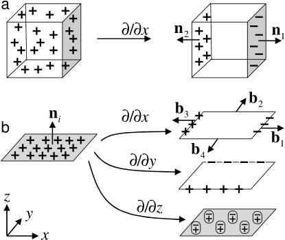
Figure 1: A sketch of modification of the “charge distribution” by taking derivatives of the potential: (a) transformation of a volume charge into a surface charge, (b) transformation of a surface charge into a linear charge and a dipole layer.

In order to find second derivatives $\partial^{2}\varphi(\mathbf{r})/\partial x_{\alpha}\partial x_{\beta}$, we note that the first derivative can be expressed as a sum over faces of the inclusion surface:

$$\frac{\partial\varphi(\mathbf{r})}{\partial\mathbf{r}}=-\sum_{\stackrel{{\scriptstyle\scriptstyle i}}{{\mathrm{(faces)}}}}\mathbf{n}^{i}\,\mathcal{F}_{i}(\mathbf{r})$$ (7)

(see Fig. 1a). Indeed, this derivative can be rewritten as

$$\frac{\partial\varphi(\mathbf{r})}{\partial\mathbf{r}}=\frac{\partial}{\partial\mathbf{r}}\int\frac{\chi(\mathbf{r}^{\prime})}{|\mathbf{r}-\mathbf{r}^{\prime}|}\,d\mathbf{r}^{\prime}=\int\frac{\partial\chi(\mathbf{r}^{\prime})}{\partial(\mathbf{r}^{\prime})}\,\frac{d\mathbf{r}^{\prime}}{|\mathbf{r}-\mathbf{r}^{\prime}|}\,.$$ (8)

The derivative $\partial\chi(\mathbf{r}^{\prime})/\partial\mathbf{r}^{\prime}$ plays the role of a “charge density” in Eq. (8). It vanishes everywhere except the surface of the inclusion. Near the $i$-th face of the surface, $\chi(\mathbf{r})$ is equal to $-\theta(\mathbf{n}^{i}(\mathbf{r}-\mathbf{r}_{i}))$, where $\mathbf{r}_{i}$ is any point of this face, $\theta$ is the Heaviside function; consequently $\partial\chi(\mathbf{r})/\partial\mathbf{r}=-\mathbf{n}^{i}\,\delta(\mathbf{n}^{i}(\mathbf{r}-\mathbf{r}_{i}))$, that corresponds to the “surface charge density” $-\mathbf{n}^{i}$ at the $i$-th face. Therefore, a contribution of the $i$-th face to $\partial\varphi(\mathbf{r})/\partial\mathbf{r}$ is equal to $-\mathbf{n}^{i}\mathcal{F}_{i}$, according to Eq. (7).

The next step is finding of derivatives of $\mathcal{F}_{i}(\mathbf{r})$. Let, for simplicity, the $i$-th face lie in the plane $XY$, and its outward normal vector $\mathbf{n}^{i}$ be directed along the axis $Z$. To find derivatives $\partial\mathcal{F}_{i}/\partial x$ and $\partial\mathcal{F}_{i}/\partial y$, one can follow the same line of argumentation as at deriving Eq. (7). The result is:

$$\frac{\partial\mathcal{F}_{i}}{\partial x}=-\sum_{k}b^{k}_{x}\Phi_{k},\quad\frac{\partial\mathcal{F}_{i}}{\partial y}=-\sum_{k}b^{k}_{y}\Phi_{k},$$ (9)

where $k$ runs over edges surrounding the $i$-th face; $\mathbf{b}^{k}$ is a unit vector which is parallel to the $i$-th face, directed out of this face, and perpendicular to the $k$-th edge (see Fig. 1b). The last derivative, $\partial\mathcal{F}_{i}/\partial z$, transforms an uniformly charhed $i$-th face into a dipole layer with surface density of dipole momentum equal to $-\mathbf{n}^{i}$, as shown in Fig. 1b. Consequently,

$$\frac{\partial\mathcal{F}_{i}}{\partial z}=-n^{i}_{z}\Omega_{i}.$$ (10)

Eqs. (9) and (10) can be written together in a vector form, which is independent on orientation of a face with respect to co-ordinate axes:

$$\frac{\partial\mathcal{F}_{i}(\mathbf{r})}{\partial\mathbf{r}}=-\mathbf{n}^{i}\Omega_{i}(\mathbf{r})-\sum_{k}\mathbf{b}^{k}\Phi_{k}(\mathbf{r}).$$ (11)

Using Eqs. (7) and (11), one can express second derivatives of the potential $\varphi(\mathbf{r})$ via solid angles $\Omega_{i}(\mathbf{r})$ and potentials of charged edges $\Phi_{k}(\mathbf{r})$:

$$\frac{\partial^{2}\varphi(\mathbf{r})}{\partial x_{\alpha}\,\partial x_{\beta}} = \sum_{\stackrel{{\scriptstyle\scriptstyle i}}{{\mathrm{(faces)}}}}n^{i}_{\alpha}n^{i}_{\beta}\,\Omega_{i}(\mathbf{r})$$ (12)

$$+ \sum_{\stackrel{{\scriptstyle\scriptstyle k}}{{\mathrm{(edges)}}}}(n^{k1}_{\alpha}b^{k1}_{\beta}+n^{k2}_{\alpha}b^{k2}_{\beta})\,\Phi_{k}(\mathbf{r}),$$

where for each edge $k$ there are four unit vectors $\mathbf{n}^{k1}$, $\mathbf{b}^{k1}$, $\mathbf{n}^{k2}$, $\mathbf{b}^{k2}$, related to the two faces intersecting at this edge. With given normals $\mathbf{n}^{k1}$ and $\mathbf{n}^{k2}$, the vectors $\mathbf{b}^{k1}$ and $\mathbf{b}^{k2}$ can be found in the following way:

$$\mathbf{b}^{k1}=\mathbf{n}^{k1}\times\mathbf{l}^{k},\qquad\mathbf{b}^{k2}=-\mathbf{n}^{k2}\times\mathbf{l}^{k},$$ (13)

where $\mathbf{l}^{k}$ is a unit vector directed along edge $k$. From two possible directions of $\mathbf{l}^{k}$, one should choose the one going clockwise with respect to face $k1$ and, correspondingly, counter-clockwise with respect to $k2$, when seeing from the outside of the inclusion.

III General solution and its properties

III.1 The general solution

In the previous Section, it was shown that the strain tensor $\varepsilon_{\alpha\beta}(\mathbf{r})$ can be expressed (via Eq. (5)) in terms of second derivatives of some auxiliary “electrostatic potential” $\varphi(\mathbf{r})$. In turn, these second derivatives break down into contributions of all faces and edges of the inclusion surface (Eq. (12)). Combining equations (5) and (12), we obtain the following expression for the strain tensor:

$$\varepsilon_{\alpha\beta}(\mathbf{r})= - \Lambda\sum_{\stackrel{{\scriptstyle\scriptstyle i}}{{\mathrm{(faces)}}}}n_{\alpha}^{i}n_{\beta}^{i}\Omega_{i}(\mathbf{r})$$ (14)

$$- \Lambda\sum_{\stackrel{{\scriptstyle\scriptstyle k}}{{\mathrm{(edges)}}}}\gamma_{\alpha\beta}^{k}\Phi_{k}(\mathbf{r})-\varepsilon_{0}\delta_{\alpha\beta}\chi(\mathbf{r}),$$

where $i$ runs over faces of the inclusion surface, and $k$ runs over its edges.

In Eq. (14), $\Omega_{i}(\mathbf{r})$ is a solid angle subtended by the $i$-th face from the point $\mathbf{r}$ (positive if the outer side of the face is seen from the point $\mathbf{r}$, and negative otherwise); $\Phi_{k}(\mathbf{r})$ is the electrostatic potential of an uniformly charged $k$-th edge (with unit linear charge density) at the point $\mathbf{r}$; $\chi(\mathbf{r})$ is equal to 1 inside the inclusion and to 0 outside it; $\varepsilon_{0}$ is the relative lattice mismatch between the inclusion and the matrix; the constant $\Lambda$ is equal to $\varepsilon_{0}(1+\nu)/4\pi(1-\nu)$, where $\nu$ is the Poisson ratio; $\delta_{\alpha\beta}$ is the Kroneker delta; $\mathbf{n}^{i}$ is a normal unit vector to the $i$-th face, directed outside the inclusion; and a constant tensor $\gamma_{\alpha\beta}^{k}$ is equal to

$$\gamma_{\alpha\beta}^{k}=n_{\alpha}^{k1}b_{\beta}^{k1}+n_{\alpha}^{k2}b_{\beta}^{k2}.$$ (15)

In Eq. (15), $\mathbf{n}^{k1}$ and $\mathbf{n}^{k2}$ are normal unit vectors (directed outside the inclusion) to the two faces which intersect at the $k$-th edge; $\mathbf{b}^{k1}$ is a unit vector perpendicular to the $k$-th edge and to $\mathbf{n}^{k1}$, and directed out of the $k1$-th face; analogously, $\mathbf{b}^{k2}$ is a unit vector perpendicular to the $k$-th edge and to $\mathbf{n}^{k2}$, directed out of the $k2$-th face (see Eq. (13)).

The tensor $\gamma_{\alpha\beta}^{k}$ is symmetrical, and it can be written in an equivalent form

$$\gamma_{\alpha\beta}^{k}=\left(A_{\alpha}^{k}A_{\beta}^{k}-B_{\alpha}^{k}B_{\beta}^{k}\right)\sin\theta,$$

where

$$\mathbf{A}^{k}=\frac{\mathbf{n}^{k1}+\mathbf{n}^{k2}}{|\mathbf{n}^{k1}+\mathbf{n}^{k2}|},\quad\mathbf{B}^{k}=\frac{\mathbf{n}^{k1}-\mathbf{n}^{k2}}{|\mathbf{n}^{k1}-\mathbf{n}^{k2}|},$$

and $\theta$ is the internal dihedral angle between faces $k1$ and $k2$.

There is a simple expression (6) for potentials $\Phi_{k}(\mathbf{r})$ contributing into Eq. (14). Some closed-form expressions for solid angles $\Omega_{i}(\mathbf{r})$ are presented in the Appendix.

Equation (14) is the main result of the present paper. It gives a closed-form analytical expression for strain distribution in and around a polyhedral inclusion buried into infinite isotropic elastic medium.

With a known strain tensor, one can easily obtain the stress tensor $\sigma_{\alpha\beta}$ via Hooke’s law: Landau

$$\sigma_{\alpha\beta}(\mathbf{r})=\frac{E}{1+\nu}\left(\varepsilon_{\alpha\beta}(\mathbf{r})+\frac{\nu}{1-2\nu}\varepsilon_{\gamma\gamma}(\mathbf{r})\delta_{\alpha\beta}\right),$$ (16)

where $E$ is the Young modulus.

On the basis of Eq. (14), the program code is written that can easily calculate the strain distribution produced by a lattice-mismatched inclusion in an infinite, isotropic matrix. Inclusion shape can be an arbitrary polyhedron. This program, named “easystrain”, is freely available at http://easystrain.narod.ru.

III.2 Cuboidal inclusion

If the inclusion has the form of cuboid with faces perpendicular to the direction of the axes $x$, $y$ and $z$ (Fig. 2), then separate components of Eq. (14) are simplified to

$$\varepsilon_{xx}(\mathbf{r}) = -\Lambda\left(\Omega_{1}(\mathbf{r})+\Omega_{2}(\mathbf{r})\right)-\varepsilon_{0}\chi(\mathbf{r}),$$

$$\varepsilon_{xy}(\mathbf{r}) = -\Lambda\left(\Phi_{1}(\mathbf{r})-\Phi_{2}(\mathbf{r})+\Phi_{3}(\mathbf{r})-\Phi_{4}(\mathbf{r})\right),$$

and all the other components of strain tensor have a similar form. So, the diagonal components $\varepsilon_{xx}$, $\varepsilon_{yy}$ and $\varepsilon_{zz}$ depend only on solid angles $\Omega_{i}$, whereas off-diagonal components $\varepsilon_{xy}$, $\varepsilon_{xz}$ and $\varepsilon_{yz}$ depend only on edge contributions $\Phi_{k}$. This is in agreement with results of Downes, Faux and O’Reilly. Downes1997_cuboid These authors pointed out that, in the case of cuboidal inclusion, solid angles subtended by faces contribute into the stress tensor (and hence into the strain tensor too). Our paper generalizes this observation to the case of any polyhedral inclusion.

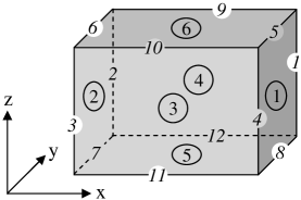
Figure 2: Cuboidal inclusion. Numbers in circles refer to faces, italic numbers refer to edges.

III.3 Hydrostatic strain

Now we consider some simple properties of the solution (14). These properties can be regarded as tests of validity of the solution.

First, let us calculate the hydrostatic component of strain (that is, the trace $\varepsilon_{\alpha\alpha}(\mathbf{r})$ of the strain tensor). Taking into account that $n^{i}_{\alpha}n^{i}_{\alpha}=(\mathbf{n}^{i})^{2}=1$, $\gamma_{\alpha\alpha}^{k}=\mathbf{n}^{k1}\mathbf{b}^{k1}+\mathbf{n}^{k2}\mathbf{b}^{k2}=0$, and $\delta_{\alpha\alpha}=3$, we readily get from Eq. (14)

$$\varepsilon_{\alpha\alpha}(\mathbf{r})=-\Lambda\sum_{i}\Omega_{i}(\mathbf{r})-3\varepsilon_{0}\chi(\mathbf{r}).$$

The sum of solid angles, $\sum_{i}\Omega_{i}(\mathbf{r})$, vanishes for any point $\mathbf{r}$ outside the inclusion. Indeed, all faces can be divided into two groups with regard to the point $\mathbf{r}$: 1) the ones whose outer sides are seen from the point $\mathbf{r}$, 2) the ones whose inner sides are seen from $\mathbf{r}$. Net solid angles subtended by the two groups are the same, but they contribute to the sum $\sum_{i}\Omega_{i}(\mathbf{r})$ with opposite signs and therefore cancel each other.

If the point $\mathbf{r}$ is inside the inclusion, all the faces belong to the second group and the solid angle subtended by them together are the full solid angle, $4\pi$. So, $\sum_{i}\Omega_{i}(\mathbf{r})=-4\pi$. Combining both cases ($\mathbf{r}$ outside and inside the inclusion) we get

$$\sum_{i}\Omega_{i}(\mathbf{r})=-4\pi\chi(\mathbf{r}),$$ (17)

and consequently

$$\varepsilon_{\alpha\alpha}(\mathbf{r})=(4\pi\Lambda-3\varepsilon_{0})\chi(\mathbf{r})=-2\varepsilon_{0}\frac{1-2\nu}{1-\nu}\chi(\mathbf{r}).$$ (18)

We have come to the well-known result that the hydrostatic strain is zero outside the inclusion and is constant inside it. Davies1998

III.4 Strain discontinuities at faces

Then, it is easy to examine the behavior of the strain at the inclusion surface, starting from Eq. (14). When the point $\mathbf{r}$, moving from outside toward inside, crosses a face of the inclusion, the strain changes stepwise. The discontinuity of the strain, $\Delta\varepsilon_{\alpha\beta}\equiv\varepsilon_{\alpha\beta}^{\mathrm{inside}}-\varepsilon_{\alpha\beta}^{\mathrm{outside}}$, can be written as

$$\Delta\varepsilon_{\alpha\beta}=-\Lambda\sum_{i}n_{\alpha}^{i}n_{\beta}^{i}\Delta\Omega_{i}-\Lambda\sum_{k}\gamma_{\alpha\beta}^{k}\Delta\Phi_{k}-\varepsilon_{0}\delta_{\alpha\beta}.$$

There $\Delta\Omega_{i}$ and $\Delta\Phi_{k}$ denote discontinuities of $\Omega_{i}$ and $\Phi_{k}$. In fact, edge contributions $\Phi_{k}$ have no discontinuities at the face, and only one of $\Omega_{i}$ has a discontinuity—namely, the $\Omega_{i}$ related to the face under consideration. For this face, $\Delta\Omega_{i}=-4\pi$, because the solid angle $|\Omega_{i}|$ reaches $2\pi$ at the face, and the value $\Omega_{i}$ changes the sign from positive to negative. So,

$$\Delta\varepsilon_{\alpha\beta}=4\pi\Lambda n_{\alpha}n_{\beta}-\varepsilon_{0}\delta_{\alpha\beta}=\varepsilon_{0}\left(\frac{1+\nu}{1-\nu}\,n_{\alpha}n_{\beta}-\delta_{\alpha\beta}\right),$$

with a unit vector $\mathbf{n}$ perpendicular to the face. It is convenient to consider the strain tensor with respect to the coordinate axes $\xi$, $\eta$, $\zeta$ connected to the face: axes $\xi$ and $\eta$ parallel to the face, and the axis $\zeta$ perpendicular to it. Therefore $n_{\xi}=n_{\eta}=0$, $n_{\zeta}=1$, and $\Delta\varepsilon_{\alpha\beta}$ takes the following form:

$$\Delta\varepsilon_{\xi\xi}=\Delta\varepsilon_{\eta\eta}=-\varepsilon_{0},\quad\Delta\varepsilon_{\zeta\zeta}=\frac{2\varepsilon_{0}\nu}{1-\nu},$$ (19)

off-diagonal components $\Delta\varepsilon_{\xi\eta}$, $\Delta\varepsilon_{\xi\zeta}$, $\Delta\varepsilon_{\eta\zeta}$ are zero. According to Hooke’s law (16), discontinuities of the stress tensor, $\Delta\sigma_{\alpha\beta}$, are

$$\Delta\sigma_{\xi\xi}=\Delta\sigma_{\eta\eta}=-\frac{E}{1-\nu},\quad\Delta\sigma_{\zeta\zeta}=0,$$ (20)

and again off-diagonal components are zero.

Equations (19) and (20) are in accordance to the boundary conditions at the interface: $\Delta\varepsilon_{\xi\xi}=\Delta\varepsilon_{\eta\eta}=-\varepsilon_{0}$, $\Delta\varepsilon_{\xi\eta}=0$ (continuity of displacement field $\mathbf{u}(\mathbf{r})$), $\Delta\sigma_{\xi\zeta}=\Delta\sigma_{\eta\zeta}=\Delta\sigma_{\zeta\zeta}=0$ (balance of elastic forces at the interface).

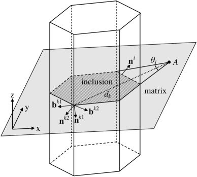
Figure 3: Quantum wire inclusion. Point $A$ is the point where the strain is to be obtained. $\theta_{i}$ and $d_{k}$ are the angle and distance contributing to Eq. (21).

III.5 Quantum-wire inclusion

Next, we consider the strain distribution in a quantum-wire-like inclusion and its surrounding (Fig. 3). Such an inclusion is a prism, the top and bottom of which go to infinity. For simplicity, let all side faces and edges be parallel to the axis $z$. So the strain is independent on $z$.

To obtain the strain distribution, one may start from Eq. (14) for a prism of finite height, and then go to the limit of infinitely large vertical dimension. In this limit, contributions of base and bottom faces, as well as of edges adjoining to these faces, vanish. For each side face, the solid angle $\Omega_{i}$ reduces to a doubled plane angle $\theta_{i}$ (Fig. 3) subtended by the cross-section of this face by a plane parallel to axes $x$, $y$: $\Omega_{i}=2\theta_{i}$. Edge contributions $\Phi_{k}$ reduce to simple logarithmic expressions:

$$\Phi_{k}=-2\log d_{i}+\mathrm{const},$$

where $d_{k}$ is the distance to the $k$-th edge (Fig. 3). The constants in these expressions are infinitely large, but they cancel each other being substituted into Eq. (14).

As a result, we come to the following expression for the strain in a quantum-wire-like inclusion:

$$\varepsilon_{\alpha\beta}(\mathbf{r})= - 2\Lambda\sum_{i}n_{\alpha}^{i}n_{\beta}^{i}\theta_{i}$$ (21)

$$+ 2\Lambda\sum_{k}\gamma_{\alpha\beta}^{k}\log d_{k}-\varepsilon_{0}\delta_{\alpha\beta}\chi.$$

There the indices $i$ and $k$ run over all side faces and edges, correspondingly; $\theta_{i}$ is the plane angle subtended by the cross section of $i$-th face by the plane passing through the point $\mathbf{r}$ parallel to the axes $x$ and $y$ (positive if the outer side of the face is seen from the point $\mathbf{r}$, and negative otherwise); $d_{k}$ is the distance from the point $\mathbf{r}$ to $k$-th edge. All the rest notations are the same as in Eq. (14). As the $xz$-, $yz$- and $zz$-components of the tensors $n^{i}_{\alpha}n^{i}_{\beta}$ and $\gamma_{\alpha\beta}^{k}$ are zero, the corresponding components of strain tensor are independent on $\theta_{i}$ and $d_{k}$:

$$\varepsilon_{xz}=\varepsilon_{yz}=0,\quad\varepsilon_{zz}=-\varepsilon_{0}\chi.$$

Equation (21) is an equivalent, but more simple and compact, form of the solution obtained by Faux, Downes and O’Reilly. Faux1997_wire

III.6 Semi-infinite matrix

Finally we discuss the strain distribution in a semi-infinite matrix. Davies Davies2003_semi_inf proposed a method of reducing the elastic inclusion problem in a semi-infinite matrix to the corresponding problem in an infinite matrix. For convenience, we reproduce there the results of Davies’s work. Davies2003_semi_inf

Let an inclusion be buried in a semi-infinite matrix that fill a half-space $z>z_{s}$, or $z<z_{s}$, with a free surface in the plane $z=z_{s}$. Isotropic linear elasticity is assumed, and elastic moduli of the matrix and the inclusion are the same. To calculate the strain distribution $\tilde{\varepsilon}_{\alpha\beta}(\mathbf{r})$ in this system, one can previously find an analogous strain distribution $\varepsilon_{\alpha\beta}(\mathbf{r})$ in a system consisting of the same inclusion in an infinite matrix. It can be found by Eq. (14), for example. Then, components of $\tilde{\varepsilon}_{\alpha\beta}(\mathbf{r})$ are expressed via components of $\varepsilon_{\alpha\beta}(\mathbf{r})$, $\varepsilon_{\alpha\beta}(\mathbf{r}_{2})$ and their derivatives $\partial\varepsilon_{\alpha\beta}/\partial z(\mathbf{r}_{2})$, where the point $\mathbf{r}_{2}$ is a “mirror image” of the point $\mathbf{r}$ with respect to the surface:

$$\mathbf{r} = (x,y,z),\quad\mathbf{r}_{2}=(x,y,2z_{s}-z),$$

$$\tilde{\varepsilon}_{xx}(\mathbf{r}) = \varepsilon_{xx}(\mathbf{r})+(3-4\nu)\varepsilon_{xx}(\mathbf{r}_{2})+2(z-z_{s})\frac{\partial\varepsilon_{xx}}{\partial z}(\mathbf{r}_{2}),$$

$$\tilde{\varepsilon}_{yy}(\mathbf{r}) = \varepsilon_{yy}(\mathbf{r})+(3-4\nu)\varepsilon_{yy}(\mathbf{r}_{2})+2(z-z_{s})\frac{\partial\varepsilon_{yy}}{\partial z}(\mathbf{r}_{2}),$$

$$\tilde{\varepsilon}_{zz}(\mathbf{r}) = \varepsilon_{zz}(\mathbf{r})-(1-4\nu)\varepsilon_{zz}(\mathbf{r}_{2})+2(z-z_{s})\frac{\partial\varepsilon_{zz}}{\partial z}(\mathbf{r}_{2}),$$

$$\tilde{\varepsilon}_{xy}(\mathbf{r}) = \varepsilon_{xy}(\mathbf{r})+(3-4\nu)\varepsilon_{xy}(\mathbf{r}_{2})+2(z-z_{s})\frac{\partial\varepsilon_{xy}}{\partial z}(\mathbf{r}_{2}),$$

$$\tilde{\varepsilon}_{xz}(\mathbf{r}) = \varepsilon_{xz}(\mathbf{r})-\varepsilon_{xz}(\mathbf{r}_{2})-2(z-z_{s})\frac{\partial\varepsilon_{xz}}{\partial z}(\mathbf{r}_{2}),$$

$$\tilde{\varepsilon}_{yz}(\mathbf{r}) = \varepsilon_{yz}(\mathbf{r})-\varepsilon_{yz}(\mathbf{r}_{2})-2(z-z_{s})\frac{\partial\varepsilon_{yz}}{\partial z}(\mathbf{r}_{2}).$$

If the inclusion is a polyhedron, Eq. (14) provides an analytical expression for the strain tensor $\varepsilon_{\alpha\beta}$. Therefore its derivative $\partial\varepsilon_{\alpha\beta}/\partial z$ can be evaluated analytically as a combination of derivatives of solid angles $\Omega_{i}$ and values $\Phi_{k}$. It is important to note that derivatives of $\Omega_{i}$ can be expressed via derivatives of $\Phi_{k}$:

$$\frac{\partial\Omega_{i}(\mathbf{r})}{\partial x_{\alpha}}=\sum_{k}\left(b^{ki}_{\alpha}n^{i}_{\beta}-b^{ki}_{\beta}n^{i}_{\alpha}\right)\frac{\partial\Phi_{k}(\mathbf{r})}{\partial x_{\beta}},$$ (22)

where summation is over all the edges adjoining to the $i$-th face; and $\mathbf{b}^{ki}$ is the one of unit vectors $\mathbf{b}^{k1}$, $\mathbf{b}^{k2}$, which is perpendicular to $\mathbf{n}^{i}$. Eq. (22) may be useful since analytical expressions for solid angles are rather complicated in comparison with the expression (6) for values $\Phi_{k}$.

IV Application to pyramidal and hut-cluster inclusions

Among all polyhedrons, the three ones appear most often as geometrical models of quantum dots. These are square-based pyramid (Fig. 4a), truncated square-based pyramid (Fig. 4b), and so-called “hut-cluster” (Fig. 4c). In this Section, we apply the general expression (14) to the specific cases of pyramidal and hut-cluster inclusions. The case of truncated pyramid does not demand a special consideration, because it is easy to obtain solution for truncated pyramid, provided that the solution for pyramid has yet been obtained (see below).

IV.1 Pyramid

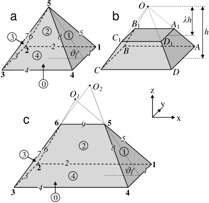
Figure 4: Inclusions of most common shapes: (a) a pyramid with square base; (b) a truncated pyramid with square base; (c) a “hut-cluster”. Numbers in circles refer to faces (the base has the number 0), italic numbers refer to edges, and bold numbers—to vertices.

With the numbering scheme of Fig. 4a, we get the following expressions for tensors $n^{i}_{\alpha}n^{i}_{\beta}$ and $\gamma_{\alpha\beta}^{k}$:

$$n_{\alpha}^{0}n_{\beta}^{0} = \left\{0,\,0,\,1,\,0,\,0,\,0\right\},$$

$$n_{\alpha}^{1}n_{\beta}^{1} = \left\{s^{2},\,0,\,c^{2},\,0,\,-sc,\,0\right\},$$

$$n_{\alpha}^{2}n_{\beta}^{2} = \left\{0,\,s^{2},\,c^{2},\,0,\,0,\,-sc\right\},$$

$$n_{\alpha}^{3}n_{\beta}^{3} = \left\{s^{2},\,0,\,c^{2},\,0,\,sc,\,0\right\},$$

$$n_{\alpha}^{4}n_{\beta}^{4} = \left\{0,\,s^{2},\,c^{2},\,0,\,0,\,sc\right\},$$

$$\gamma_{\alpha\beta}^{1} = s\times\left\{c,\,0,\,-c,\,0,\,-s,\,0\right\},$$

$$\gamma_{\alpha\beta}^{2} = s\times\left\{0,\,c,\,-c,\,0,\,0,\,-s\right\},$$

$$\gamma_{\alpha\beta}^{3} = s\times\left\{c,\,0,\,-c,\,0,\,s,\,0\right\},$$

$$\gamma_{\alpha\beta}^{4} = s\times\left\{0,\,c,\,-c,\,0,\,0,\,s\right\},$$

$$\gamma_{\alpha\beta}^{5} = s/\sqrt{1+c^{2}}\times\left\{-c^{2},\,-c^{2},\,2c^{2},\,1,\,sc,\,sc\right\},$$

$$\gamma_{\alpha\beta}^{6} = s/\sqrt{1+c^{2}}\times\left\{-c^{2},\,-c^{2},\,2c^{2},\,-1,\,-sc,\,sc\right\},$$

$$\gamma_{\alpha\beta}^{7} = s/\sqrt{1+c^{2}}\times\left\{-c^{2},\,-c^{2},\,2c^{2},\,1,\,-sc,\,-sc\right\},$$

$$\gamma_{\alpha\beta}^{8} = s/\sqrt{1+c^{2}}\times\left\{-c^{2},\,-c^{2},\,2c^{2},\,-1,\,sc,\,-sc\right\},$$

where $s=\sin\vartheta$, $c=\cos\vartheta$, and $\vartheta$ is a dihedral angle between the pyramid base and any of its side face. The tensor components are listed in braces in the following order: $xx$, $yy$, $zz$, $xy$, $xz$, $yz$.

It is worth to note the following property of the set of tensors $\gamma_{\alpha\beta}^{k}$:

$$\sum_{k}\gamma_{\alpha\beta}^{k}L_{k}=0,$$

where $L_{k}$ is the length of the $k$-th edge. This property comes from a requirement that all terms proportional to $r^{-1}$ in Eq. (14) must cancel each other at $r\rightarrow\infty$. It may serve as a useful test of correctness of the results.

These values of $n^{i}_{\alpha}n^{i}_{\beta}$ and $\gamma_{\alpha\beta}^{k}$, together with Eq. (14), give the expression for the strain distribution in a pyramidal inclusion and its surrounding:

$$\varepsilon_{xx} = -s^{2}\Lambda(\Omega_{1}+\Omega_{3})-sc\Lambda(\Phi_{1}+\Phi_{3})+\textstyle\frac{sc^{2}\Lambda}{\sqrt{1+c^{2}}}\Phi_{5-8}-\varepsilon_{0}\chi,$$

$$\varepsilon_{yy} = -s^{2}\Lambda(\Omega_{2}+\Omega_{4})-sc\Lambda(\Phi_{2}+\Phi_{4})+\textstyle\frac{sc^{2}\Lambda}{\sqrt{1+c^{2}}}\Phi_{5-8}-\varepsilon_{0}\chi,$$

$$\varepsilon_{zz} = -\Lambda\Omega_{0}-c^{2}\Lambda\Omega_{1-4}+sc\Lambda\Phi_{1-4}-\textstyle\frac{2sc^{2}\Lambda}{\sqrt{1+c^{2}}}\Phi_{5-8}-\varepsilon_{0}\chi,$$ (23)

$$\varepsilon_{xy} = -\textstyle\frac{s\Lambda}{\sqrt{1+c^{2}}}(\Phi_{5}-\Phi_{6}+\Phi_{7}-\Phi_{8}),$$

$$\varepsilon_{xz} = sc\Lambda(\Omega_{1}-\Omega_{3})+s^{2}\Lambda(\Phi_{1}-\Phi_{3})-\textstyle\frac{s^{2}c\Lambda}{\sqrt{1+c^{2}}}(\Phi_{5}-\Phi_{6}-\Phi_{7}+\Phi_{8}),$$

$$\varepsilon_{yz} = sc\Lambda(\Omega_{2}-\Omega_{4})+s^{2}\Lambda(\Phi_{2}-\Phi_{4})-\textstyle\frac{s^{2}c\Lambda}{\sqrt{1+c^{2}}}(\Phi_{5}+\Phi_{6}-\Phi_{7}-\Phi_{8}).$$

There we use a shorthand notation: $\Omega_{1-4}=\Omega_{1}+\Omega_{2}+\Omega_{3}+\Omega_{4}$, and so on. Note that, using Eq. (17), one can simplify the expression for $\varepsilon_{zz}$ to the following one:

$$\varepsilon_{zz} = -s^{2}\Lambda\Omega_{0}+sc\Lambda\Phi_{1-4}$$ (24)

$$-\textstyle\frac{2sc^{2}\Lambda}{\sqrt{1+c^{2}}}\Phi_{5-8}+\varepsilon_{0}(c^{2}\textstyle\frac{1+\nu}{1-\nu}-1)\chi.$$

Eq. (A) in the Appendix provides analytical expressions for solid angles $\Omega_{0}...\Omega_{4}$ in the pyramid.

IV.2 Truncated pyramid

To get the solution for the truncated pyramid, $\varepsilon_{\alpha\beta}^{\mathrm{(trunc)}}$, the easiest way is to start from the solution for a pyramid, $\varepsilon_{\alpha\beta}^{\mathrm{(pyr)}}$, and apply the superposition principle. The full pyramid, $OABCD$, consists of a truncated one, $ABCDA_{1}B_{1}C_{1}D_{1}$, and a smaller one, $OA_{1}B_{1}C_{1}D_{1}$ (Fig. 4b). According to the superposition principle,

$$\varepsilon_{\alpha\beta}^{\mathrm{(pyr)}}(\mathbf{r})=\varepsilon_{\alpha\beta}^{\mathrm{(trunc)}}(\mathbf{r})+\varepsilon_{\alpha\beta}^{\mathrm{(small)}}(\mathbf{r}),$$

where $\varepsilon_{\alpha\beta}^{\mathrm{(pyr)}}$, $\varepsilon_{\alpha\beta}^{\mathrm{(trunc)}}$ and $\varepsilon_{\alpha\beta}^{\mathrm{(small)}}$ refer to figures $OABCD$, $ABCDA_{1}B_{1}C_{1}D_{1}$ and $OA_{1}B_{1}C_{1}D_{1}$, correspondingly. Then, it is well known that, in the framework of the continual elasticity theory, similar inclusions produce similar strain fields. As pyramids $OABCD$ and $OA_{1}B_{1}C_{1}D_{1}$ are similar, there is a relation between $\varepsilon_{\alpha\beta}^{\mathrm{(pyr)}}$ and $\varepsilon_{\alpha\beta}^{\mathrm{(small)}}$:

$$\varepsilon_{\alpha\beta}^{\mathrm{(pyr)}}(\mathbf{r}_{O}+\mathbf{r})=\varepsilon_{\alpha\beta}^{\mathrm{(small)}}(\mathbf{r}_{O}+\lambda\mathbf{r}),$$

where $\mathbf{r}_{O}$ is a position vector of the apex $O$, $\lambda$ is a truncation parameter (a ratio of sizes of the two pyramids, see Fig. 4b). So $\varepsilon_{\alpha\beta}^{\mathrm{(trunc)}}$ can be expressed in terms of $\varepsilon_{\alpha\beta}^{\mathrm{(pyr)}}$:

$$\varepsilon_{\alpha\beta}^{\mathrm{(trunc)}}(\mathbf{r})=\varepsilon_{\alpha\beta}^{\mathrm{(pyr)}}(\mathbf{r})-\varepsilon_{\alpha\beta}^{\mathrm{(pyr)}}(\frac{\mathbf{r}-\mathbf{r}_{O}}{\lambda}+\mathbf{r}_{O}).$$ (25)

This solution was compared numerically with the solution published in Ref. Pearson2000_pyramid, . We reproduce all strain profiles presented in that paper, except the component $\varepsilon_{xz}$ in Fig. 11 of Ref. Pearson2000_pyramid, , where the absolute value coincides with our results, but the sign was opposite. We believe that the sign of $\varepsilon_{xz}$ in Ref. Pearson2000_pyramid, is erroneous, because it leads to an incorrect behavior of the strain at $r\rightarrow\infty$. Indeed, the multipole expansion, being applied to Eq. (1), gives for large $r$

$$\varepsilon_{\alpha\beta}(\mathbf{r}+\mathbf{r}_{c})=\frac{\varepsilon_{0}V(1+\nu)}{4\pi(1-\nu)}\;\frac{\delta_{\alpha\beta}-3r_{\alpha}r_{\beta}/r^{2}}{r^{3}}+O(r^{-5}),$$

where $V$ is a volume of the inclusion, and $\mathbf{r}_{c}$ is a position vector of its center of mass. For a pyramid, $x_{c}=y_{c}=0$. This expression shows that, at fixed positive $x$ and $y$, $\varepsilon_{xz}$ must be negative when $z\rightarrow+\infty$ and positive when $z\rightarrow-\infty$. This predicted behavior of $\varepsilon_{xz}$ disagrees with Fig. 11 of Ref. Pearson2000_pyramid, , but agrees with our calculations.

IV.3 Hut-cluster

Finally, we consider the hut-cluster. The hut-cluster is a figure that consists of the base (a parallelogram) and four side faces. Slope angles of all the side faces are the same. Therefore orientations of faces and edges of the hut-cluster are the same as of pyramid, except the top (9th) edge. So, the solution for the hut-cluster is very similar to the one for the pyramid. The only difference is the addition of the contribution of 9th edge. Of course, the values of solid angles $\Omega_{0}...\Omega_{4}$ and of edge contributions $\Phi_{1}...\Phi_{8}$ in the hut-cluster are not the same as in the pyramid. Analytical expressions for solid angles in the hut-cluster are given by Eq. (A) in the Appendix.

To get the solution for the hut-cluster from Eq. (IV.1), it is sufficient to add the term $2sc\Lambda\Phi_{9}$ to $\varepsilon_{yy}$, and to add the term $-2sc\Lambda\Phi_{9}$ to $\varepsilon_{zz}$. This demonstrates the flexibility of the general solution (14). This is a property that is not inherent in previous particular solutions. Pearson2000_pyramid ; Glas2001 ; Stoleru2002_pyramid

An analytical solution for a hut-cluster was first obtained by GlasGlas2001 as a special case of a more general answer for a truncated pyramid with rectangular bottom and top faces. Our method provides a much more simple solution.

IV.4 Strain profiles along axes of symmetry

If the point $\mathbf{r}$ lies at the four-fold axis of symmetry of the pyramid, expressions (IV.1) are simplified greatly, because all values $\Omega_{1}(\mathbf{r})...\Omega_{4}(\mathbf{r})$ are the same, values $\Phi_{1}(\mathbf{r})...\Phi_{4}(\mathbf{r})$ are the same, and $\Phi_{5}(\mathbf{r})...\Phi_{8}(\mathbf{r})$ are also the same. Moreover, it is sufficient to evaluate only the $zz$-component of the strain, because non-diagonal components $\varepsilon_{xy}$, $\varepsilon_{xz}$, $\varepsilon_{yz}$ are zero, and other diagonal components $\varepsilon_{xx}$ and $\varepsilon_{yy}$ can be expressed via $\varepsilon_{zz}$ using Eq. (18):

$$\varepsilon_{xx}=\varepsilon_{yy}=\frac{1}{2}(\varepsilon_{\alpha\alpha}-\varepsilon_{zz})=-\varepsilon_{0}\frac{1-2\nu}{1-\nu}\chi-\frac{1}{2}\varepsilon_{zz}.$$ (26)

It is convenient to use Eq. (24) for evaluation the component $\varepsilon_{zz}$. Let us put the origin of coordinate system to the center of the pyramid base. So, coordinates of a point at the axis of symmetry are $(0,0,z)$. Let $h$ be a pyramid height, $a$ be a length of the pyramid base, $l=\sqrt{a^{2}/2+h^{2}}$ be a length of a side edge, and $r$ be a distance between the point $(0,0,z)$ and any vertex of the pyramid base:

$$r=\sqrt{a^{2}/2+z^{2}}.$$

According to Eq. (A), the solid angle $\Omega_{0}$ is equal to

$$\Omega_{0}=-4\arctan\frac{a^{2}}{4zr}.$$

Then,

$$\Phi_{1}=\Phi_{2}=\Phi_{3}=\Phi_{4} = \log\frac{2r+a}{2r-a},$$

$$\Phi_{5}=\Phi_{6}=\Phi_{7}=\Phi_{8} = \log\frac{|z-h|+r+l}{|z-h|+r-l}.$$

Substituting all these quantities into Eq. (24), we get

$$\varepsilon_{zz}(0,0,z) = \frac{8ah\Lambda}{a^{2}+4h^{2}}\left(\frac{2h}{a}\arctan\frac{a^{2}}{4zr}+\log\frac{2r+a}{2r-a}\right.$$ (27)

$$- \left.\frac{a}{l}\log\frac{|z-h|+r+l}{|z-h|+r-l}\right)+\tilde{\Lambda}\chi.$$

Here we expressed quantities $s$ and $c$ in terms of $a$, $h$, and $l$; $\Lambda=\varepsilon_{0}(1+\nu)/4\pi(1-\nu)$; $\chi=1$ if $z\in(0;h)$ and $\chi=0$ otherwise; the constant $\tilde{\Lambda}$ is the coefficient at $\chi$ in Eq. (24):

$$\tilde{\Lambda}=\varepsilon_{0}(c^{2}\textstyle\frac{1+\nu}{1-\nu}-1)\equiv\varepsilon_{0}\left(\frac{a^{2}(1+\nu)}{(a^{2}+4h^{2})(1-\nu)}-1\right).$$

For the truncated pyramid, Eq. (25) together with Eq. (27) give

$$\!\!\!\!\!\!\!\!\varepsilon_{zz}(0,0,z)=\frac{8ah\Lambda}{a^{2}+4h^{2}}\left(\frac{2h}{a}\arctan\frac{a^{2}}{4zr}-\frac{2h}{a}\arctan\frac{a^{2}}{4\tilde{z}\tilde{r}}\right.$$

$$\!\!\!\!\!\!\!\!+\left.\log\!\frac{(2r\!+\!a)(2\tilde{r}\!-\!a)}{(2r\!-\!a)(2\tilde{r}\!+\!a)}-\frac{a}{l}\log\!\frac{\lambda\tilde{r}\!+\!r\!+\!(1\!-\!\lambda)l}{\lambda\tilde{r}\!+\!r\!-\!(1\!-\!\lambda)l}\right)\!+\!\tilde{\Lambda}\chi.$$ (28)

In Eq. (IV.4), $\chi=1$ if $z\in(0;(1-\lambda)h)$, and $\chi=0$ otherwise; $\tilde{z}=(z-h)/\lambda+h$; $\tilde{r}=\sqrt{a^{2}/2+\tilde{z}^{2}}$ is a distance between the point $(0,0,\tilde{z})$ and any vertex of the base; $l=\sqrt{a^{2}/2+h^{2}}$.

In a similar manner, one can get the strain profile along the axis of symmetry of the hut-cluster. As there is only two-fold axis in the hut-cluster, the components $\varepsilon_{xx}$ and $\varepsilon_{yy}$ are no longer the same. Therefore we cannot use Eq. (26) to extract $\varepsilon_{xx}$ and $\varepsilon_{yy}$ from $\varepsilon_{zz}$. Instead, we should find $\varepsilon_{zz}$ and $\varepsilon_{xx}$ independently, and then extract $\varepsilon_{yy}$ by means of Eq. (18):

$$\varepsilon_{yy}=\varepsilon_{\alpha\alpha}-\varepsilon_{xx}-\varepsilon_{zz}=-2\varepsilon_{0}\frac{1-2\nu}{1-\nu}\chi-\varepsilon_{xx}-\varepsilon_{zz}.$$

We chose the center of the cluster base as an origin of the coordinate system. Let $h$ be a cluster height, $a$ and $b$ be the smaller and the bigger edge lengths of the base, correspondingly. Then, values of $\varepsilon_{zz}$ and $\varepsilon_{xx}$ at the axis of symmetry are

$$\varepsilon_{zz}(0,0,z)\!=\!\frac{8ah\Lambda}{a^{2}\!+\!4h^{2}}\left(\frac{2h}{a}\arctan\frac{ab}{4zr_{1}}+\frac{1}{2}\log\frac{(2r_{1}\!+\!a)(2r_{1}\!+\!b)}{(2r_{1}\!-\!a)(2r_{1}\!-\!b)}-\frac{a}{l}\log\frac{r_{5}\!+\!r_{1}\!+\!l}{r_{5}\!+\!r_{1}\!-\!l}-\frac{1}{2}\log\frac{2r_{5}\!+\!(b\!-\!a)}{2r_{5}\!-\!(b\!-\!a)}\right)+\tilde{\Lambda}\chi,$$ (29)

$$\varepsilon_{xx}(0,0,z)\!=\!\frac{8ah\Lambda}{a^{2}\!+\!4h^{2}}\!\left(\!-\frac{2h}{a}\arctan\frac{a^{2}z-abh}{[b(b\!-\!a)\!+\!4z(z\!-\!h)]r_{1}\!+\!(b^{2}\!+\!4z^{2})r_{5}}-\!\frac{1}{2}\log\frac{2r_{1}\!+\!a}{2r_{1}\!-\!a}+\!\frac{a}{2l}\log\frac{r_{5}\!+\!r_{1}\!+\!l}{r_{5}\!+\!r_{1}\!-\!l}\right)-\varepsilon_{0}\chi,$$ (30)

where $r_{1}(z)=\sqrt{a^{2}/4+b^{2}/4+z^{2}}$ is a distance from the point $(0,0,z)$ to the first vertex of the hut-cluster; $r_{5}(z)=\sqrt{(b-a)^{2}/4+(z-h)^{2}}$ is a distance from the point $(0,0,z)$ to the fifth vertex; $l=\sqrt{a^{2}/2+h^{2}}$ is a length of each side edge; $\chi=1$ if $z\in(0;h)$ and $\chi=0$ otherwise. The last log term in Eq. (29) is a contribution of the 9th edge, and the arctangent term in Eq. (30) comes from the first and the third faces. All the rest terms are similar to that of Eq. (27).

Figure 5: The strain component, $\varepsilon_{zz}$, plotted along the $z$ axis for a pyramid (Eq. (27), solid line), a truncated pyramid (Eq. (IV.4), dash line), and a hut-cluster (Eq. (29), dash-dot line).

As an illustration, in Fig. 5 we plotted profiles of the strain component, $\varepsilon_{zz}$, calculated by Equations (27–29) for some particular cases of pyramidal, truncated pyramidal, and hut-cluster inclusions. Parameters of the structures are chosen to be the same as ones in Ref. Pearson2000_pyramid, : $\varepsilon_{0}=0.067$; $\nu=0.24$; $a=155$ Å; $h=55$ Å for the pyramid and the hut-cluster; $h=110$ Å and $\lambda=0.5$ for the truncated pyramid; $b=2a$ for the hut-cluster. Presented curves for the pyramid and the truncated pyramid are identical to ones of Ref. Pearson2000_pyramid, (curves D and B in Fig. 5, correspondingly), that confirms the correctness of our formulas.

A detailed discussion of these profiles is beyond the scope of the present paper. We only note that $\varepsilon_{zz}$ diverges logarithmically at $z=55$ Å in the pyramid and the hut-cluster. This divergence is a common feature of a strain distribution in a vicinity of a vertex or an edge of any polyhedral inclusion.

V Elastic anisotropy

The above consideration was based on an assumption of elastically isotropic inclusion and matrix. For applications to semiconductor heterostructures, this assumption may be a source of considerable error. For example, the Young modulus of silicon in $\langle 111\rangle$ direction is 1.44 times greater than that in $\langle 100\rangle$ direction. Therefore, taking the elastic anisotropy into account is an actual problem.

In this Section, we argue that our method can be expanded to anisotropic media. We start from expression of strain tensor via Green’s tensor $G_{\alpha\beta}$ by Faux and Pearson Faux2000_expansion :

$$\varepsilon_{\alpha\beta}(\mathbf{r})=\varepsilon_{0}\int_{V}G_{\alpha\beta}(\mathbf{r}-\mathbf{r}^{\prime})d\mathbf{r}^{\prime},$$

where $V$ is the inclusion volume, and $\varepsilon_{0}$ is lattice mismatch. These authors found a series expansion for Green’s tensor, assuming cubic anisotropy:

$$G_{\alpha\beta}=G_{\alpha\beta}^{(0)}+\Delta G_{\alpha\beta}^{(1)}+\Delta^{2}G_{\alpha\beta}^{(2)}+...\,,$$ (31)

where expansion coefficient $\Delta=(C_{11}-C_{12}-2C_{44})/(C_{12}+2C_{44})$ is a measure of anisotropy ($\Delta\approx-\frac{1}{3}$ for typical semiconductors), $C_{11}$, $C_{12}$ and $C_{44}$ are elastic moduli. Each term of this expansion can be presented as a combination of partial derivatives of expressions like $1/r$, $x^{2}/r$, etc. For example, isotropic term is

$$G_{\alpha\beta}^{(0)}(\mathbf{r})=-\frac{\varepsilon_{0}}{4\pi}\,\frac{3C_{12}+2C_{44}}{C_{12}+2C_{44}}\,\frac{\partial^{2}}{\partial x_{\alpha}\partial x_{\beta}}\,\frac{1}{r}\,;$$

$xx$-component of first-order correction, $G_{xx}^{(1)}$, is a linear combination of the following terms:

$$\frac{\partial^{2}}{\partial x^{2}}\,\frac{1}{r},\quad\frac{\partial^{3}}{\partial x^{3}}\,\frac{x}{r},\quad\frac{\partial^{4}}{\partial x^{4}}\,\frac{x^{2}}{r},\quad\frac{\partial^{4}}{\partial x^{2}\partial y^{2}}\,\frac{y^{2}}{r},\quad\frac{\partial^{4}}{\partial x^{2}\partial z^{2}}\,\frac{z^{2}}{r}.$$

As a result, strain tensor $\varepsilon_{\alpha\beta}({\mathbf{r}})$ expresses as a combination of derivatives

$$\frac{\partial^{\,a+b+c}}{\partial x^{a}\,\partial y^{b}\,\partial z^{c}}\int_{V}(x^{\prime})^{d}(y^{\prime})^{e}(z^{\prime})^{f}\frac{d\mathbf{r}^{\prime}}{\mathbf{r}-\mathbf{r}^{\prime}}\,,$$ (32)

where $a,b,c,d,e,f=0,1,2,...$ with a constraint $a+b+c=d+e+f+2$. Each term in the expansion (31) is a sum of a finite number of derivatives (32) taken with proper constant coefficients.

According to our method, the integrals in Eq. (32) can be regarded as electrostatic potentials induced by a non-uniformly charged inclusion. Taking the derivatives in Eq. (32), one proceeds from “volume charge” to “surface dipoles” on faces of the inclusion surface, and to “linear charges” and “multipoles” on its edges. Thus, our method allows to split the strain tensor into contributions of faces and edges of inclusion surface (assuming that inclusion shape is a polyhedron):

$$\varepsilon_{\alpha\beta}(\mathbf{r})=\sum_{i}A_{\alpha\beta}^{(i)}(\mathbf{r})+\sum_{k}B_{\alpha\beta}^{(k)}(\mathbf{r}),$$ (33)

where indices $i$ and $k$ run over all faces and edges, correspondingly.

Explicit formulas for contributions $A_{\alpha\beta}^{(i)}$ and $B_{\alpha\beta}^{(k)}$ are beyond the scope of the present paper and are the subject of a separate publication. There we only note that each face contribution $A_{\alpha\beta}^{(i)}(\mathbf{r})$ is proportional to a solid angle $\Omega_{i}(\mathbf{r})$ with a coefficient depending on the orientation of this face and on elastic constants. Edge contributions $B_{\alpha\beta}^{(k)}(\mathbf{r})$ can be expressed in a closed form for each term of series expansion (31).

VI Conclusions

In summary, we propose a new, more simple and flexible expression for strain field in and around an inclusion buried in an infinite or semi-infinite isotropic medium. This expression was also implemented as a computer program.easystrain We show that the strain field can be presented as a sum of contributions of the faces and edges. This is the main point of our method; it gives a possibility to construct expressions for strain distribution in inclusions of complicated shapes. The general solution is applied to important particular cases of pyramidal and hut-cluster inclusions. Our solution for the pyramid reproduces previous solutions, but in a simpler and intuitively understandable form. We believe that it paves the way for further simplifications and generalizations of the solution, for example, to the case of anisotropic elasticity.

Appendix A Evaluation of solid angles

Here we present some explicit formulas expressing solid angles as functions of coordinates.

A solid angle $\Omega(\mathbf{r})$, that a surface $S$ subtends at a point $\mathbf{r}$, may be defined as an integral over the surface:

$$\Omega(\mathbf{r})=\int\limits_{S}\frac{\mathbf{n}(\mathbf{r}-\mathbf{r}^{\prime})}{|\mathbf{r}-\mathbf{r}^{\prime}|^{3}}\,dS,$$ (34)

where $dS$ is a surface element, $\mathbf{n}$ is a unit vector directed normally to this surface element, and $\mathbf{r}^{\prime}$ is a position vector of the surface element.

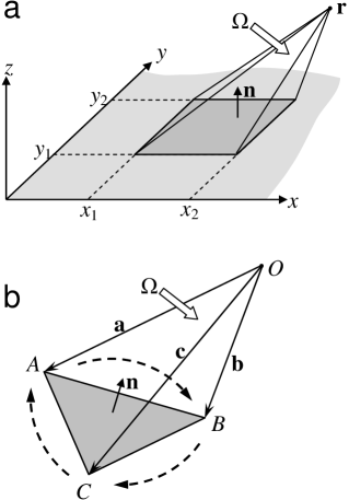
Figure 6: Solid angles: (a) expressed by Eq. (35); (b) expressed by Eq. (37).

This integral is easily evaluated if the surface $S$ is a rectangle. For simplicity, let this rectangle lie in the plane $z=0$, and its edges be oriented along the axes $x$ and $y$ (Fig. 6a). Let $x_{1}$ and $x_{2}$ be $x$-coordinates of edges directed along the axis $y$ $(x_{1}<x_{2})$; $y_{1}$ and $y_{2}$ be $y$-coordinates of the rest two edges of the rectangle $(y_{1}<y_{2})$. Then the integral (34) is expressed as follows:

$$\Omega^{\mathrm{rect}}(\mathbf{r};x_{1},x_{2},y_{1},y_{2})=\int\limits_{x_{1}}^{x_{2}}\!\!dx^{\prime}\!\!\!\int\limits_{y_{1}}^{y_{2}}\!\!\!\frac{dy^{\prime}\,z}{((x\!-\!x^{\prime})^{2}\!+\!(y\!-\!y^{\prime})^{2}\!+\!z^{2})^{3/2}},$$

or

$$\Omega^{\mathrm{rect}}(\mathbf{r};x_{1},x_{2},y_{1},y_{2})=$$ (35)

$$\textstyle\arctan\frac{(x-x_{1})(y-y_{1})}{z\,r_{11}}-\arctan\frac{(x-x_{1})(y-y_{2})}{z\,r_{12}}-$$

$$\textstyle\arctan\frac{(x-x_{2})(y-y_{1})}{z\,r_{21}}+\arctan\frac{(x-x_{2})(y-y_{2})}{z\,r_{22}}.$$

Here $r_{11}...r_{22}$ are distances from the point $\mathbf{r}$ to the corners of the rectangle:

$$\scriptstyle r_{11}=\sqrt{(x-x_{1})^{2}+(y-y_{1})^{2}+z^{2}},\quad r_{12}=\sqrt{(x-x_{1})^{2}+(y-y_{2})^{2}+z^{2}},$$

$$\scriptstyle r_{21}=\sqrt{(x-x_{2})^{2}+(y-y_{1})^{2}+z^{2}},\quad r_{22}=\sqrt{(x-x_{2})^{2}+(y-y_{2})^{2}+z^{2}}.$$

It is assumed that values of arctangents fall into the range $(-\frac{\pi}{2},+\frac{\pi}{2})$.

To find a solid angle subtended by a triangle (Fig. 6b), one can use the relation by Oosterom and Strackee: Oosterom_solid ; wiki_solid

$$\tan\!\frac{\Omega^{\mathrm{triangle}}(\mathbf{a},\!\mathbf{b},\!\mathbf{c})}{2}=\frac{[\mathbf{a}\times\mathbf{b}]\,\mathbf{c}}{abc\!+\!(\mathbf{a}\mathbf{b})c\!+\!(\mathbf{a}\mathbf{c})b\!+\!(\mathbf{b}\mathbf{c})a}.$$ (36)

Vectors $\mathbf{a}$, $\mathbf{b}$, $\mathbf{c}$ join the point $O$, at which the solid angle is subtended, to the vertices $A$, $B$, $C$ of the triangle. To satisfy the condition that the solid angle $\Omega$ is positive if it is looked at from outside, and is negative otherwise, one should choose the proper order of following of the vertices $A$, $B$, $C$. Namely, the closed contour $ABCA$ should follow in a clockwise direction, seeing from outside the inclusion (as shown by dashed arrows in Fig. 6b). So the triple scalar product $[\mathbf{a}\times\mathbf{b}]\,\mathbf{c}$ is positive (negative) if the outer (inner) side of the triangular face is seen from the point $O$.

Care must be taken while resolving Eq. (36) with respect to $\Omega$. For simplicity, we will refer to the right side of Eq. (36) as to $\lambda$. The sign of $\Omega$ is the same as the sign of the product $[\mathbf{a}\times\mathbf{b}]\,\mathbf{c}$, but may differ from the sign of $\lambda$. So we cannot “naively” resolve Eq. (36) as $\Omega=2\arctan\lambda$. Instead, we should write down $\Omega=2(\arctan\lambda\;\mathrm{mod}\;\pi)$ if $[\mathbf{a}\times\mathbf{b}]\,\mathbf{c}>0$, and $\Omega=2(\arctan\lambda\;\mathrm{mod}\;\pi)-2\pi$ otherwise. Joining together both cases, we obtain

$$\Omega^{\mathrm{triangle}}(\mathbf{a},\!\mathbf{b},\!\mathbf{c})$$ (37)

$$= 2\left(\arctan\frac{[\mathbf{a}\times\mathbf{b}]\,\mathbf{c}}{abc\!+\!(\mathbf{a}\mathbf{b}\!)c\!+\!(\mathbf{a}\mathbf{c}\!)b\!+\!(\mathbf{b}\mathbf{c}\!)a}\,\mathrm{mod}\,\pi\right)$$

$$- 2\pi\left(1-\theta([\mathbf{a}\times\mathbf{b}]\,\mathbf{c})\right),$$

where $\theta(x)$ is the Heaviside function (1 for positive $x$, 0 for negative $x$). Note that the easiest way to implement Eq. (37) in a computer program is to use C math library function atan2: $\Omega=2*\mathrm{atan2}(P,Q)$, where $P$ and $Q$ are numerator and denominator of the right part of Eq. (36).

With Eq. (37), one can calculate a solid angle subtended by an arbitrary polygon, breaking this polygon down into triangles.

Now let us apply the expressions (35) and (37) to faces of the pyramid and the hut-cluster considered in Section IV. First, we choose a reference frame with the origin at the center of the pyramid base, the axes $x$ and $y$ along edges of the base, and the axis $z$ directed toward the apex of the pyramid. So, position vectors of the vertices (see Fig. 4a) are

$$\mathbf{r}_{1} \!=\! (a/2,a/2,0),\;\mathbf{r}_{2}=(-a/2,a/2,0),$$

$$\mathbf{r}_{3} \!=\! (-a/2,-a/2,0),\;\mathbf{r}_{4}=(a/2,-a/2,0),\;\mathbf{r}_{5}=(0,0,h),$$

where $a$ is a base edge length, $h$ is a height of the pyramid. Note that a dihedral angle $\vartheta=\arctan(2h/a)$. Solid angles contributing into Eq. (IV.1) are

$$\Omega_{0}(\mathbf{r}) = -\Omega^{\mathrm{rect}}\textstyle(\mathbf{r};-\frac{a}{2},\frac{a}{2},-\frac{a}{2},\frac{a}{2}),$$

$$\Omega_{1}(\mathbf{r}) = \Omega^{\mathrm{triangle}}(\mathbf{r}_{1}-\mathbf{r},\mathbf{r}_{4}-\mathbf{r},\mathbf{r}_{5}-\mathbf{r}),$$

$$\Omega_{2}(\mathbf{r}) = \Omega^{\mathrm{triangle}}(\mathbf{r}_{2}-\mathbf{r},\mathbf{r}_{1}-\mathbf{r},\mathbf{r}_{5}-\mathbf{r}),$$ (38)

$$\Omega_{3}(\mathbf{r}) = \Omega^{\mathrm{triangle}}(\mathbf{r}_{3}-\mathbf{r},\mathbf{r}_{2}-\mathbf{r},\mathbf{r}_{5}-\mathbf{r}),$$

$$\Omega_{4}(\mathbf{r}) = \Omega^{\mathrm{triangle}}(\mathbf{r}_{4}-\mathbf{r},\mathbf{r}_{3}-\mathbf{r},\mathbf{r}_{5}-\mathbf{r}).$$

The minus sign at $\Omega^{\mathrm{rect}}$ in Eq. (A) reflects the fact that the pyramid base is directed downwards.

For the hut-cluster, position vectors of vertices are

$$\mathbf{r}_{1} \!=\! (b/2,a/2,0),\;\mathbf{r}_{2}=(-b/2,a/2,0),$$

$$\mathbf{r}_{3} \!=\! (-b/2,-a/2,0),\;\mathbf{r}_{4}=(b/2,-a/2,0),$$

$$\mathbf{r}_{5} \!=\! ((b-a)/2,0,h),\;\mathbf{r}_{6}=(-(b-a)/2,0,h).$$

Here $a$ and $b$ are the smaller and the bigger edge lengths of the base. (Again, the dihedral angle is $\vartheta=\arctan(2h/a)$.) We introduce also two points $O_{1}$ and $O_{2}$ where side edges cross (see Fig. 4b):

$$\mathbf{r}_{O_{1}}=(0,-(b-a)/2,hb/a),\;\mathbf{r}_{O_{2}}=(0,(b-a)/2,hb/a).$$

The solid angle $\Omega_{2}$ of the trapezoidal 2nd face is the difference of two solid angles subtended by triangles $O_{1}12$ and $O_{1}56$. The angle $\Omega_{4}$ is evaluated in the same way. As a result, solid angles subtended by faces of the hut-cluster are

$$\Omega_{0}(\mathbf{r}) = -\Omega^{\mathrm{rect}}\textstyle(\mathbf{r};-\frac{b}{2},\frac{b}{2},-\frac{a}{2},\frac{a}{2}),$$

$$\Omega_{1}(\mathbf{r}) = \Omega^{\mathrm{triangle}}(\mathbf{r}_{1}-\mathbf{r},\mathbf{r}_{4}-\mathbf{r},\mathbf{r}_{5}-\mathbf{r}),$$

$$\Omega_{2}(\mathbf{r}) = \Omega^{\mathrm{triangle}}(\mathbf{r}_{2}-\mathbf{r},\mathbf{r}_{1}-\mathbf{r},\mathbf{r}_{O_{1}}-\mathbf{r})$$ (39)

$$- \Omega^{\mathrm{triangle}}(\mathbf{r}_{6}-\mathbf{r},\mathbf{r}_{5}-\mathbf{r},\mathbf{r}_{O_{1}}-\mathbf{r}),$$

$$\Omega_{3}(\mathbf{r}) = \Omega^{\mathrm{triangle}}(\mathbf{r}_{3}-\mathbf{r},\mathbf{r}_{2}-\mathbf{r},\mathbf{r}_{6}-\mathbf{r}),$$

$$\Omega_{4}(\mathbf{r}) = \Omega^{\mathrm{triangle}}(\mathbf{r}_{4}-\mathbf{r},\mathbf{r}_{3}-\mathbf{r},\mathbf{r}_{O_{2}}-\mathbf{r})$$

$$- \Omega^{\mathrm{triangle}}(\mathbf{r}_{5}-\mathbf{r},\mathbf{r}_{6}-\mathbf{r},\mathbf{r}_{O_{2}}-\mathbf{r}).$$

These expressions can be substituted into a modified version of Eq. (IV.1), as described in Section IV.

References

- (1) G. L. Bir and G. E. Pikus, Symmetry and Strain-Induced Effects in Semiconductors (Wiley, New York, 1974).
- (2) C. G. Van de Walle, Phys. Rev. B 39, 1871 (1989).
- (3) A. V. Dvurechenskii, A. V. Nenashev, and A. I. Yakimov, Nanotechnology 13, 75 (2002).
- (4) J. Stangl, V. Holý, and G. Bauer, Rev. Mod. Phys. 76, 725 (2004).
- (5) R. Maranganti and P. Sharma, Handbook of Theoretical and Computational Nanotechnology, Chapter 118 (2006).
- (6) M. Grundmann, O. Stier, and D. Bimberg, Phys. Rev. B 52, 11969 (1995).
- (7) C. Pryor, Phys. Rev. B 57, 7190 (1998).
- (8) O. Stier, M. Grundmann, and D. Bimberg, Phys. Rev. B 59, 5688 (1999).
- (9) S. Christiansen, M. Albrecht, H. P. Strunk, and H. J. Maier, Appl. Phys. Lett. 64, 3617 (1994).
- (10) S. Noda, T. Abe, and M. Tamura, Phys. Rev. B 58 7181 (1998).
- (11) M. A. Cusack, P. R. Briddon, and M. Jaros, Phys. Rev. B 54, R2300 (1996).
- (12) A. V. Nenashev and A. V. Dvurechenskii, Zh. Eksp. Teor. Fiz. 118, 570 (2000) [Engl. transl. JETP 91, 497 (2000)].
- (13) Y. Kikuchi, H. Sugii, and K. Shintani, J. Appl. Phys. 89, 1191 (2001).
- (14) I. Daruka, A.-L. Barabasi, S. J. Zhou, T. C. Germann, P. S. Lomdahl, and A. R. Bishop, Phys. Rev. B 60, R2150 (1999).
- (15) D. A. Faux, J. R. Downes, and E. P. O’Reilly, J. Appl. Phys. 80, 2515 (1996).
- (16) J. R. Downes, D. A. Faux, and E. P. O’Reilly, J. Appl. Phys. 81, 6700 (1997).
- (17) V. G. Stoleru, D. Pal, and E. Towe, Physica E 15, 131 (2002).
- (18) A. D. Andreev, J. R. Downes, D. A. Faux, and E. P. O’Reilly, J. Appl. Phys. 86, 297 (1999).
- (19) F. Glas, J. Appl. Phys. 90, 3232 (2001).
- (20) J. D. Eshelby, Proc. R. Soc. London, Ser. A 241, 376 (1957).
- (21) J. H. Davies, J. Appl. Phys. 84, 1358 (1998).
- (22) G. S. Pearson and D. A. Faux, J. Appl. Phys. 88, 730 (2000).
- (23) D. A. Faux, J. R. Downes, and E. P. O’Reilly, J. Appl. Phys. 82, 3754 (1997).
- (24) H. Nozaki and M. Taya, J. Appl. Mech. 68, 441 (2001).
- (25) J. H. Davies, J. Appl. Mech. 70, 655 (2003).
- (26) I. E. Tamm, Fundamentals of the Theory of Electricity (Mir, Moscow, 1979), p. 82.
- (27) L. D. Landau and E. M. Lifshitz, Theory of Elasticity.
- (28) D.A. Faux and G.S. Pearson, Phys. Rev. B 62, 4798 (2000).
- (29) http://easystrain.narod.ru
- (30) A. Van Oosterom and J. Strackee, IEEE Trans. on Biomed. Eng. 30, 125 (1983).
- (31) http://en.wikipedia.org/wiki/Solid_angle