Dynamical localization of a particle coupled to a two-level systems thermal reservoir

Abstract

Using the functional-integral method, we investigate the effect of a two-level systems thermal reservoir on the single particle dynamics. We find that at low temperatures, within the sub-ohmic regime, the particle becomes “dynamically” localized at long times due to an effective potential generated by the particle-reservoir interaction. This behavior is different from the one obtained for the usual bath of harmonic oscillators and is fundamentally related with the non-Markovian character of the dissipative process.

I Introduction

The influence of dissipation on quantum tunnelingAOannal and on quantum coherenceAJLrmodphy has attracted much attention during the last decades. In a pioneer work, Caldeira and LeggettAOannal suggested that a bosonic heat bath consisting of an infinite number of harmonic oscillators constitutes an universal realization, which can mimic a large variety of real environments.Weiss However, a real environment cannot always be represented in this way. Indeed, if the particle of interest couples to a non linear system, the latter may, under certain circumstances, behave as a fermionic heat bath. That is the case of a distribution of quartic plus quadratic potentials, which within a very well known limit,quartic effectively acts as a collection of two-level systems (TLSs). In such a case the environment truly behaves as a spin $1/2$ medium.

A spin-bath composed of an infinite number of TLSs has been mostly considered when the system of interest is itself a TLS, PSrepprphy providing for instance, a realistic description of a nanomagnet coupled to a set of surrounding spinsMagTunn and a useful model to describe the loss of quantum coherence.Hangi ; Makri The representation of dissipative environments by a spin-bath has been extended also to situations in which the environment is not composed of real spins, as e.g. in the description of disordered insulating solidstwlinsu or for explaining the damping of acoustic phonons in a nanomechanical resonator.ressonator Moreover, it has been found that the dissipative dynamics of a single particle linearly coupled to a TLSs reservoir is non-MarkoviantwlAHCN and that the transport properties strongly differ from the usual oscillator thermal bath.twlyo Indeed, the optical conductivity of a set of non interacting particles linearly coupled to a TLSs reservoir exhibits a remarkable non-Drude behavior. In particular, in the sub-ohmic regime the system exhibits a maximum in the incoherent electrical conductivity at finite frequency.twlyo This kind of behavior has been experimentally observed in La_2-xSr_xCuO₄takenaka1 and La_1-xSrMnO₃,takenaka2 in situations in which inelastic scattering dominates the transport properties. The broad finite energy peak observed experimentally suggests a "dynamical" localization of the charged particles, similar to the non-Fermi-liquid behavior found in the infrared conductivity of SrRuO₃.kostic In all the cases discussed above, the localization of the particle was attributed to inelastic scattering processes because they are strongly enhanced as the temperature is raised. This high-temperature localization is different from the Anderson localization, which tends to be destroyed by inelastic processes.

In this paper we present a simple model, which leads to “dynamical” localization due to inelastic scattering, but at low temperatures. At this point, we want to call the attention of the reader to our use of the term “dynamical” localization. This term is conventionally used in the literaturedynamical to designate quantum phenomena taking place in time-periodic systems, whose corresponding classical dynamics displays chaotic diffusion. The phenomenon described here bears no similarities with the latter and for this reason we use the term under quotation marks. The “dynamical” localization of the charge carriers studied here is generated by their coupling to a TLSs thermal bath and is in close relation to a non-Markovian process at the classical level. At first sight, a non-Markovian particle dynamics, which implies that the particle never reaches equilibrium, seems to be in contradiction with localization, which is characteristic of insulators. This paper intends also to shed some light on this point. In order to achieve our goal, we investigate the real time effective dynamics of a single particle coupled to a TLSs thermal reservoir in the sub-ohmic regime. The effective action, which describes the particle interacting with the TLSs bath, is obtained using the well known Feynman-Vernon formalism.FeyVer

This paper is divided as follows: In Sec. II we present the model describing the particle of interest interacting with the TLSs reservoir, as well as a brief sketch of the derivation of the effective particle dynamics. In Sec. III the “dynamical” localization effect is explicitly derived and discussed in specific cases within the sub-ohmic regime. Finally in Sec. IV we present our conclusions.

II The Model

To begin with, we will describe the particle of interest coupled to a generic TLSs thermal reservoir by the Hamiltonian

$$H=\frac{{\hat{p}}^{2}}{2M}+u(x)+\sum_{k=1}^{N}\frac{{\hbar\omega_{k}}}{2}\sigma_{zk}-x\sum_{k=1}^{N}J_{k}\sigma_{xk},$$ (1)

where the first two terms stand for a particle under the influence of an arbitrary potential $u$, the third term accounts for the TLSs reservoir, and the last one describes the interaction between the particle and the thermal bath. $J_{k}$ denotes the coupling parameter and $\sigma_{zk/xk}$ stand for Pauli matrices.

The first step is to calculate the reduced density operator of the particle of interest, which may be obtained after tracing out the reservoir degrees of freedom,

$$\rho(x,y,t)={\textrm{Tr}}_{R}[\langle x|e^{-i\frac{{Ht}}{\hbar}}\rho(0)e^{i\frac{{Ht}}{\hbar}}|y\rangle].$$ (2)

The density operator of the total system at time $t=0$ will be assumed to be decoupled, $\rho(0)=\rho_{S}(0)\rho_{R}(0)$. The reduced density operator (2) can then be written as

$$\rho(x,y,t)=\int dx^{\prime}\int dy^{\prime}\rho_{S}(x^{\prime},y^{\prime},0){\mathcal{J}}(x,y,t;x^{\prime}y^{\prime},0),$$

where the super-propagator ${\mathcal{J}}$ has the form

$${\mathcal{J}}=\int_{x^{\prime}}^{x}{\mathcal{D}}x(t^{\prime})\int_{y^{\prime}}^{y}{\mathcal{D}}y(t^{\prime})e^{\frac{{i}}{\hbar}(S_{0}[x]-S_{0}[y])}{\mathcal{F}}[x,y].$$ (3)

In the expression above, $S_{0}[x]$ corresponds to the action of a free particle placed in the potential $u$, while ${\mathcal{F}}$ denotes the influence functional which describes the influence of the reservoir on the particle dynamics. After integrating out the reservoir degrees of freedom and introducing a set of coordinates corresponding to the particle center of mass $q=(x+y)/2$ and relative coordinate $\xi=x-y$, we obtain the super-propagator for the particle of interest (see [twlyo, ] for details),

$$\mathcal{J}[q,\xi,t;q^{\prime},\xi^{\prime},0]=\int_{\xi^{\prime}}^{\xi}{\mathcal{D}}\xi\int_{q^{\prime}}^{q}{\mathcal{D}}q\>e^{\frac{{i}}{\hbar}S_{\textrm{eff}}[q,\xi]-\frac{{1}}{\hbar}\phi[\xi]}.$$ (4)

The effective action is given by

$$S_{\textrm{eff}} = \int_{0}^{t}dt^{\prime}\left[M\dot{q}(t^{\prime})\dot{\xi}(t^{\prime})-u(q,\xi)\right.$$ (5)

$$\left.-\int_{0}^{t^{\prime}}dt^{\prime\prime}\Lambda(t^{\prime}-t^{\prime\prime})q(t^{\prime\prime})\xi(t^{\prime})\right],$$

where

$$\Lambda=\int_{0}^{\infty}d\omega J(\omega,T)\sin[\omega(t^{\prime}-t^{\prime\prime})],$$

and the functional $\phi$ has the form

$$\phi[\xi]=\int_{0}^{t}dt^{\prime}\int_{0}^{t^{\prime}}dt^{\prime\prime}\Phi(t^{\prime}-t^{\prime\prime})\xi(t^{\prime})\xi(t^{\prime\prime}),$$ (6)

with

$$\Phi=\int_{0}^{\infty}d\omega J(\omega,T)\,\cos[\omega(t^{\prime}-t^{\prime\prime})]\coth\left(\hbar\omega/2k_{B}T\right).$$

It should be noticed that the kernels $\Lambda$ and $\Phi$ are both defined in terms of the spectral density of the thermal reservoirtwlyo $J(\omega,T)$.

We now perform an integration by parts to render explicit the dependence of the last term in Eq. (5) on the velocity. We then find

$$S_{\textrm{eff}} = \int_{0}^{t}dt^{\prime}\left[M\dot{\xi}(t^{\prime})\dot{q}(t^{\prime})-\xi(t^{\prime})\int_{0}^{t^{\prime}}dt^{\prime\prime}{\tilde{\Gamma}}(t^{\prime}-t^{\prime\prime})\dot{q}(t^{\prime\prime})\right.$$ (7)

$$+ \left.{\tilde{\Gamma}}(0)\xi(t^{\prime})q(t^{\prime})-u(q,\xi)-q(0){\tilde{\Gamma}}(t^{\prime})\xi(t^{\prime})\right],$$

where

$${\tilde{\Gamma}}(t^{\prime}-t^{\prime\prime})=\int_{0}^{\infty}d\omega\frac{J(\omega,T)}{\omega}\cos[\omega(t^{\prime}-t^{\prime\prime})].$$ (8)

Although in this form the effective action shows an explicit velocity dependent term, characteristic of viscous forces, we have obtained also two additional spurious contributions. The first term in the second line of Eq. (7) is nothing but a harmonic potential, which can be canceled by an appropriate choice of the external potential,

$$u(q,\xi)={\tilde{\Gamma}}(0)q\xi={\tilde{\Gamma}}(0)(x{{}^{2}}-y^{2})/2.$$

This assumption allows us to focus on the dissipative effects of the environment. An alternative procedure would be to start from a momentum dependent particle-reservoir interaction. In this way the effective action would immediately exhibit a velocity dependent term, without any additional spurious contribution. To conclude the analysis of Eq. (7) we must point out that its last term fluctuates very rapidly for times $t\gg 1/\omega$. Hence, in principle this term could be neglected within the long time regime. However, as we will show below, there is no need to introduce approximations because it will cancel out naturally when we introduce the initial conditions of the problem. The effective action for a single particle coupled to the TLSs reservoir then reads

$$S_{\textrm{eff}}[q,\xi] = \int_{0}^{t}dt^{\prime}\left[M\dot{q}(t^{\prime})\dot{\xi}(t^{\prime})-q(0){\tilde{\Gamma}}(t^{\prime})\xi(t^{\prime})\right.$$ (9)

$$\left.-\int_{0}^{t^{\prime}}dt^{\prime\prime}{\tilde{\Gamma}}(t^{\prime}-t^{\prime\prime})\dot{q}(t^{\prime\prime})\xi(t^{\prime})\right].$$

Before explicitly solving the equation of motion corresponding to the action (9), it is convenient to specify the spectral density of the thermal bath in terms of macroscopic parameters. A reasonable assumptiontwlyo for it is

$$J(\omega,T)=\frac{\eta}{\pi}\,\left(\frac{\omega}{\omega_{c}}\right)^{s}\tanh\left(\frac{\hbar\omega}{2k_{B}T}\right)\;\Theta(\Omega-\omega),$$ (10)

where $\Omega$ is a cutoff frequency, $\eta$ is a constant defining the coupling strength of the particle to the TLSs, $s$ is a number (real and positive) which determines the long time properties of the thermal bath, and $\omega_{c}$ is some characteristic frequency introduced in order to make the unit of $\eta$ independent of $s$. Notice that the temperature dependence in Eq. (10) is crucial for a fermionic heat bath because it ensures that the bath degrees of freedom are excited as the temperature increases.comentario In Ref. [Hjing, ] this point was not acknowledged, leading to the wrong conclusion that the decaying term in the particle equation of motion is temperature independent.

Using Eqs. (9) and (10), the classical equations of motion for $q$ and $\xi$ can be written as

$$\ddot{q}+\frac{2\gamma}{\pi}\int_{0}^{t}dt^{\prime}\Gamma(t-t^{\prime})\,\dot{q}(t^{\prime})+\frac{2\gamma}{\pi}q(0)\Gamma(t)=\frac{eE(t)}{M},$$ (11)

$$\ddot{\xi}-\frac{2\gamma}{\pi}\int_{0}^{t}dt^{\prime}\Gamma(t-t^{\prime})\,\dot{\xi}(t^{\prime})+\frac{2\gamma}{\pi}\xi(0)\Gamma(-t)=0,$$ (12)

where the damping constant is defined as $\gamma=\eta/2M$ and the kernel $\Gamma$ is given by

$$\Gamma(t)=\int_{0}^{\Omega}d\omega\frac{\omega^{s-1}}{\omega_{c}^{s}}\,\tanh\left(\frac{{\hbar\omega}}{2k_{B}T}\right)\cos(\omega t).$$ (13)

Therefore, after tracing out the TLSs reservoir we obtained an equation of motion for the particle center of mass (11) in which the thermal bath has the same effect as that of a viscous fluid.

For any value of $s$ the solution of Eqs. (11) and (12) can be written in terms of the kernel Laplace transform as

$$\overline{q}(z)=\frac{{zq(0)+\dot{q}(0)}}{z{{}^{2}}+2\gamma z\Gamma(z)/\pi},$$ (14)

$$\overline{\xi}(z)=\frac{{z\xi(0)+\dot{{\xi}}(0)}}{z{{}^{2}}-2\gamma z\Gamma(z)/\pi},$$ (15)

where

$$\Gamma(z) = \frac{\Omega^{s+1}}{s+1}\left[\frac{{}_{2}F_{1}(1,\frac{1+s}{2},\frac{3+s}{2},-\frac{\Omega{{}^{2}}}{z{{}^{2}}})}{z{{}^{2}}}\tan\left(\frac{\hbar z}{2kT}\right)\right.$$ (16)

$$\left.-\frac{4k_{B}Tz}{\hbar}\sum_{n=1}^{\infty}\frac{\,{}_{2}F_{1}(1,\frac{1+s}{2},\frac{3+s}{2},-\frac{\Omega{{}^{2}}}{\lambda_{n}{{}^{2}}})}{\lambda_{n}{{}^{2}}(\lambda_{n}^{2}-z{{}^{2}})}\right].$$

In the expression above ${}_{2}F_{1}$ denotes the hyper-geometric function and $\lambda_{n}=(2n-1)\pi k_{B}T/\hbar$, with $n\in\mathbb{N}$. It should be notice that the fluctuating force, given by the last term on the LHS in Eq. (11), does not appear in Eq. (14). This term was exactly canceled by the initial condition included in the Laplace transform of the damping term and therefore there is no need to drop it out by assuming the long time approximation. In order to illustrate how the dissipative properties of the TLSs thermal reservoir affects the single particle dynamics in the sub-ohmic regime ($s<1$), lets investigate the simple case in which $q(0)=0$ and $\dot{q}(0)=v_{0}$.

III The “dynamical” localization

We start by discussing the $s=0$ case, in which we can proceed analytically a bit further. In this case the hyper-geometric function reads ${}_{2}F_{1}(1,1/2,3/2,-x{{}^{2}})=x^{-1}\arctan x$ and the Laplace transform of the damping function given by Eq. (16) acquires the form

$$\Gamma=\sum_{n=1}^{\infty}\frac{4k_{B}Tz}{\hbar(\lambda_{n}^{2}-z^{2})}\left[\frac{\tan^{-1}\left(\frac{\Omega}{z}\right)}{z}-\frac{\tan^{-1}\left(\frac{\Omega}{\lambda_{n}}\right)}{\lambda_{n}}\right].$$ (17)

In the particular case of $\Omega\rightarrow\infty$, the high temperature limit of Eq. (17) is $\Gamma(z)=\hbar/2k_{B}T$ and therefore the effective dynamics of the particle of interest simply becomes

$$q(t)=\frac{v_{0}}{\hbar\gamma/2k_{B}T}(1-e^{-\frac{\hbar\gamma}{2k_{B}T}t}).$$ (18)

This result correctly reproduces the oscillator-bath model with an ohmic temperature dependent damping constant. Indeed, if we assume $\hbar\omega\ll k_{B}T$ and $\Omega\rightarrow\infty$ in Eq. (13) the damping function becomes $\Gamma(t-t^{\prime})=(\hbar\pi/2k_{B}T)\delta(t-t^{\prime})$, which is an instantaneous function, indicating that the dissipative process is completely memoryless and the condition of zero frictional force is achived only when the particle velocity is zero. Physically, this limit corresponds to a weak particle-reservoir interaction because most of the TLSs are occupied (on average), causing no damping on the particle. Therefore, we recover the known result demonstrated in Ref. [FeyVer, ], namely that when the coupling between the particle of interest and a nonlinear bath is weak enough, the latter behaves as a collection of harmonic oscillators.

However, the features discussed above are not valid for all values of temperature and frequency cutoff. In fact, we realize that at $T=0$, even assuming $\Omega\rightarrow\infty$, it is impossible to obtain a damping function without memory. In this case the problem becomes non-Markovian and although the particle becomes localized after some time, neither its position nor its velocity ever reach the equilibrium. This behavior is illustrated in Fig.1 for finite $\Omega$ and different values of temperature. It is worth to notice that in this situation the particle dynamics completely differs from its behavior in the oscillator bath model. In the later, at zero velocity, the frictional force over the particle is also zero and classically, the particle remains in that state forever. In our non-Markovian situation, the frictional force acting on the particle depends on the previous velocities with different weights - given by the kernel (13) - and the situation of zero frictional force over the particle, at a given instant, does not correspond to zero velocity.

It is not difficult to see that at low temperature, the kernel oscillates in time, keeping its sign constant and therefore the only possibility of getting zero frictional force acting on the particle at a given instant occurs when the particle changes the momentum direction within the time interval. From the physical point of view, this behavior resembles that of a particle confined by a potential. Indeed, the particle oscillation around this effective potential, which clearly appears for $T=0.0001$ in Fig. 1, can be promptly obtained within the long time regime. The term $\cos[\omega(t-t^{\prime})]$ in Eq. (13) then oscillates rapidly, yielding no contribution to the damping process for long times, except when $\omega\ll(t-t^{\prime})^{-1}$. In such a situation, $\Gamma(t)$ becomes finite and time independent, turning the damping term into a harmonic localizing potential. As the temperature increases, less reservoir states are able to play their dissipative role and the particle takes longer to get localized far from the origin.

Figure 1: Time dependence of the particle center of mass for $s=0$ and different values of temperature. The continuous line corresponds to $T=0.0001$, while the dash-dotted, dotted, dashed and double-dotted lines are for $T=0.01$, $T=0.1$, $T=0.2$ and $T=0.5$, respectively. In all cases $\Omega=1$, $\gamma=0.3$ and the initial velocity was taken equal to $1$.

We can therefore conclude that the particle dynamics in this situation ($s=0$) is completely different from the one obtained when the thermal bath is represented by the usual oscillator model. Here, memory effects in the damping process lead to a “dynamical” localization of the particle at a certain distance from the initial position, which is proportional to the temperature. The strength of the localization potential is determined by the ratio of two quantities, namely the thermal and the cutoff energies. This quantity measures the number of reservoir states which effectively couple to the particle and obviously also depends on the total reservoir states determined by the spectral function.

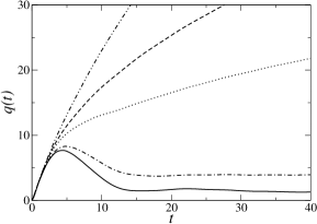
Figure 2: Time dependence of the particle center of mass for $s=0.5$ and different values of temperature. The continuous line corresponds to $T=0.0001$, while the dash-dotted, dotted, dashed and double-dotted lines are for $T=0.01$, $T=0.1$, $T=0.2$ and $T=0.5$, respectively. In all cases $\Omega=1$, $\gamma=0.3$ and the initial velocity was taken equal to $1$.

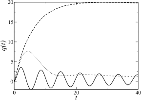
Figure 3: Time dependence of the particle center of mass for $T=0.001$ and different values of $s$. The continuous line corresponds to $s=0$, while the dotted and dashed lines are for $s=0.5$ and $s=1$, respectively. In all cases $\Omega=1$, $\gamma=0.3$ and the initial velocity was taken equal to $1$.

In order to get more insight on the particle dynamics in the sub-ohmic regime we have plotted in Fig. 2 the position as a function of time in the specific case of $s=0.5$. At very low temperatures, the main difference from the $s=0$ case is that the localizing potential strength in the long time regime becomes weaker and the dynamical localization effect is difficult to observe, see the $T=0.0001$ and $T=0.01$ cases, for instance. This is a consequence of having decreased the weight of the low energy reservoir states in the spectral function. At the same time, as the temperature increases, the number of low energy states effectively contributing to the dissipative process becomes reduced because several low-energy states are occupied (on average) and the particle moves nearly free, see Fig. 2 for $T=0.2$ and $T=0.5$. This last behavior differs from the $s=0$ situation in which, even at high temperatures, there are enough low energy states to localize the particle. In general, the particle dynamics in the sub-ohmic regime will be described by a function which exhibits a behavior in between that of the $s=0$ and $s=1$ limiting cases. This behavior is illustrated for low temperatures in Fig. 3. The central point in the ohmic case $(s=1)$ is that even at low temperatures, there are not enough low energy states that render the particle confinement appreciable in the long time regime.

IV Conclusions

We have studied the real time dynamics of a particle coupled to a TLSs thermal reservoir and found that within the sub-ohmic regime the particle becomes localized in the long time limit, oscillating in the real space as a consequence of an effective potential generated by its interaction with the thermal bath. The oscillatory behavior renders the localization “dynamical” and therefore neither the particle position nor its velocity ever reach the equilibrium. This behavior is associated with the non-Markovian character of the dissipative process, which in our simple model is provided by inelastic scattering of the particle of interest by the TLSs. We hope that our findings can be of some help in the understanding of transport properties of systems in which the dissipative medium seems to be sub-ohmic.experi ; sachdev ; dudu We also speculate about the extension of the model discussed here to a situation in which the fermionic bath excitation has a finite gap $\Delta(T)$. In such a case, we expect that the effect of “dynamical” localization will start at temperatures above $\Delta(T)/k_{B}$, which is probably more appropriate to describe realistic situations.

References

- (1) A. O. Caldeira and A. J. Leggett, Ann. Phys. (N.Y.) 149, 347 (1983).
- (2) A. J. Leggett et al, Rev. Mod. Phys. 59, 1 (1987).
- (3) U. Weiss, Quantum Dissipative Systems, 2nd ed., Series in Modern Condensed Matter Physics Vol. 10 (Singapore 1999).
- (4) A.T. Dorsey, M.P.A. Fisher, and M.S. Wartak, Phys. Rev. A 33, 1117 (1986).
- (5) N. V. Prokof’ev and P.C. E. Stamp, Rep. Prog. Phys. 63, 669 (2000).
- (6) Quantum Tunneling of Magnetization - Proceeding from the Institute of Nuclear Theory - Vol. 5 ed. by S. Tomsoviv (World Scientific, Singapore, 1998).
- (7) J. Shao and P. Hänggi, Phys. Rev. Lett. 81, 5710 (1998).
- (8) N. Makri, J. Phys. Chem. B 103, 2823 (1999).
- (9) P.W. Anderson, B.I. Halperin, and C.M. Varma, Phil. Mag. 25, 1 (1972).
- (10) C. Seoánez, F. Guinea, and A.H. Castro Neto, Europhys. Lett. 78, 60002 (2007).
- (11) A. O. Caldeira, A. H. Castro Neto, and T. Oliveira de Carvalho, Phys. Rev. B 48, 13974 (1993).
- (12) A. Villares Ferrer, A.O. Caldeira, and C. Morais Smith, Phys. Rev. B 74, 184304 (2006).
- (13) K. Takenaka, J. Nohara, R. Shiozaki, and S. Sugai, Phys. Rev. B 68 134501 (2003).
- (14) K. Takenaka, R. Shiozaki and S. Sugai, Phys. Rev. B 65, 184436 (2002).
- (15) P. Kostic et al., Phys. Rev. Lett. 81, 2498 (1998).
- (16) G. Casati et al., Lect. Notes Physics 93, 334 (1979).
- (17) R. P. Feynman and F. L. Vernon, Ann. Phys. 24, 118 (1963).
- (18) See reference [3] page 51 for a discussion concerning the relation between fermionic and bosonic spectral density functions.
- (19) Q. Dai and H. Jing, Int. J. Theor. Phys. 45, 2137 (2006).
- (20) W. Warta and N. Karl, Phys. Rev. B, 32, 1172 (1985).
- (21) D. Tanaskovic, V. Dobrosavljevic, and E. Miranda, Phys. Rev. Lett. 95, 167204 (2005).
- (22) P. Nikolic and S. Sachdev, Phys. Rev. B 73, 134511 (2006).