Anomalous thermal expansion in $\alpha$-titanium

Abstract

We provide a complete quantitative explanation for the anisotropic thermal expansion of hcp Ti at low temperature. The observed negative thermal expansion along the c-axis is reproduced theoretically by means of a parameter free theory which involves both the electron and phonon contributions to the free energy. The thermal expansion of titanium is calculated and found to be negative along the c-axis for temperatures below $\sim$ 170 K, in good agreement with observations. We have identified a saddle-point Van Hove singularity near the Fermi level as the main reason for the anisotropic thermal expansion in $\alpha-$titanium.

PACS numbers: 65.40.De, 63.20.Dj, 71.20.Be

The most general aspects of the chemical bonding in the transition $d$ metals can be understood from the Friedel modelharrison , explaining the trends in equilibrium volume, bulk modulus and cohesive energy. The transition metals are found to crystallize at low temperatures in the cubic fcc and bcc structures, and the hexagonal hcp structure footnote1 , which can be qualitatively explained from a band filling of itinerant d-statesskriver . In addition, the Debye model reproduces the thermal volume expansion with a rather good accuracymoruzzi . Hence, with a seemingly good understanding of the fundamental mechanisms governing the properties of the transition metals, the recently observed negative thermal expansion coefficient along the c-axis of one of these elements, the hcp ($\alpha$) phase of Ti Misha , stands out as an enigma. Especially since no other transition metal so far has been shown to display such a behaviour.

The problem of finding connections between the electronic structure of metals and alloys and peculiarities of their lattice properties has a long history, starting with the “third Hume-Rothery rule” concerning boundaries of phase stability in noble-metal alloys hume and its explanation by Jones in terms of touching of the Brillouin zone faces by the Fermi sphere jones (for a review of further developments of these ideas, see Ref. KNT ). The general concept of electronic topological transitions (ETT), introduced by I. Lifshitz Lif , that is, a coincidence of the Fermi level with a Van Hove singularity of the electronic density of states (DOS), is of crucial importance for understanding these interrelations. Phase transitions and pre-martensitic anomalies of elastic moduli in alkali and alkaline-earth metals under pressure provide a clear example of the effects of the Van Hove singularities on the lattice properties vaks1 ; vaks2 . It turns out that the singularity in the electron DOS at the Fermi energy, $N(E_{F})$, should be visible also in elastic moduli and Debye temperature and, thus, in the thermodynamic properties of metals at low enough temperatures (the anomalies in phonon spectra with large enough wave vectors and thus in high-temperature thermodynamic properties are in general weaker, see Ref. KNT and references therein). Since the thermal expansion is connected with the pressure derivatives of the elastic moduli, anomalies in the thermal expansion might be especially strong. In particular, it can be proven thermodynamically that ETT in non-cubic metals should lead to a singular anisotropic thermal expansion at low enough temperatures Misha ; Antropov . The latter means that in principle it is always possible to prepare a textured material with zero thermal expansion. This conclusion, being interesting in itself, opens new ways to find nonmagnetic Invar systems. However, based on these general considerations alone it is impossible to predict the temperature region where the effect should be observable, or how far from the point of ETT the effect is still visible. Here we answer these questions based on direct microscopic calculations, in a framework of the density functional theory, and we address the recently discovered negative thermal expansion of $\alpha$-Ti Misha .

The occurrence of negative thermal expansion at low temperatures for non-cubic elemental solids have been known for quite some time, but only for elements outside the transition metal series. For instance, the hexagonal close packed metals zinc and cadmium Munn have negative thermal expansion coefficients along the a-axis ($\alpha_{\bot}$) for temperatures below $\sim$ 75 K, while amongst the IIIB group of the Periodic Table it is tin and indium that have negative thermal expansion coefficients along the basal plane ($\alpha_{\bot}$) and orthogonal to the basal plane ($\alpha_{||}$), respectively Munn . Amongst the transition metals, Ti however stands out.

The analysis presented here is based on first principles density functional theory of the electron and phonon contributions to the total energy. We write the Helmholtz free energy as

$$F(\bar{\epsilon},T)=\qquad\qquad\qquad\qquad\qquad\qquad\qquad\qquad$$

$$\frac{V}{2}\sum_{ij}C_{ij}\epsilon_{i}\epsilon_{j}+F^{phon}(\bar{\epsilon},T)+F^{el}(\bar{\epsilon},T),$$ (1)

where $C_{ij}$ are the elastic constants, $\bar{\epsilon}$ the elastic strain, $V$ the volume, $F^{phon}$ the phonon free energy and $F^{el}$ the energy of thermal excitations in the electron subsystem. In this expression the reference (zero) level is for a crystal at equilibrium conditions at zero temperature. The elastic constants were calculated from first principlesmethod .

To evaluate the free energy contribution $F^{phon}$, which can be expressed as wallace ; wille

$$F^{phon}(\bar{\epsilon},T)=\qquad\qquad\qquad\qquad\qquad\qquad\qquad$$

$$\int_{0}^{\infty}d\omega g(\omega,\bar{\epsilon})[\frac{\hbar\omega}{2}+k_{B}Tln(1-e^{-\hbar\omega/k_{B}T})],$$ (2)

the phonon DOS $g(\omega,\bar{\epsilon})$ has to be calculated. This was done within the quasi-harmonic approximation YUN ; PETROS , where all anharmonic effects except the thermal expansion are neglected when calculating the temperature dependence of the phonons. In practice the phonon DOS was calculated by making small displacements of the atoms in a supercell (SC) PETROS . The directions of the displacements were $[110]$ and $[001]$ with amplitudes that were equal to $\sim$0.4% of the lattice constant. The supercell used was a 3x3x2 cell. Further details are found in Ref.method, . The energy of thermal excitations of electron states $F^{el}$ was calculated by the standard expression by Sommerfeld and Frank Sommer .

$$F^{el}(\bar{\epsilon},T)=-\frac{(\pi k_{B})^{2}}{6}D(\epsilon_{F},\bar{\epsilon})T^{2}.$$ (3)

where $D(\epsilon_{F},\bar{\epsilon})$ is the calculated electronic density of states at the Fermi level.

In Fig.1 we compare our calculated phonon spectrum (at $T=0$) with experimental values (at room temperature). It is worthwhile to mention that a tight-binding calculation of the phonon dispersion for hcp Ti has been published recently sven-ti , where parameters of the model were fitted to experimental data as well as to first principles calculations. The theoretical phonon dispersion curve in Fig.1 agrees very well with the theoretical curves in Ref. sven-ti . When comparing the theoretical and experimental Stassis curves, we note an overall agreement, although certain differences can be identified. For instance, along the $\Gamma-A$ direction the theory underestimates the frequencies in the lowest experimental branch, whereas the higher branches are reproduced with better accuracy, especially using the general gradient approximation (GGA). Also, the calculated lowest branch along the $\Gamma-K$ direction comes out somewhat too low compared to observations. The phonon DOS was then calculated with the method of Ref. Alfe .

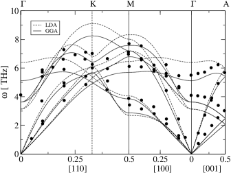
Figure 1: The phonon dispersion of hcp Ti at room temperature and ambient pressure. The solid curve is the calculated frequencies from GGA and the dashed curve represents calculated frequencies from LDA. Both calculations are done at the experimental volume $V_{0}=15.91$ų. The filled circles are the experimental data of Stassis $et$ $al$ Stassis .

By differentiating the free energy (Anomalous thermal expansion in $\alpha$-titanium) with respect to $\epsilon_{v}\equiv d(ln(V))$ and $\epsilon_{c}\equiv d(ln(c/a))$, it is possible to obtain an expression for the change in volume and structural property as a function of temperature. These changes are expressed in terms of equilibrium strains ,$\epsilon_{v}^{0}$ and $\epsilon_{c}^{0}$ at which $\partial F/\partial\epsilon_{v}=\partial F/\partial\epsilon_{c}=0$, and can be written in terms of the elastic constants and strain derivatives of the free energy

$$\epsilon_{v}^{0}(T)=\frac{1}{V(B_{11}B_{22}-B_{12}^{2})}\Big{[}-B_{22}\frac{\partial F^{*}}{\partial\epsilon_{v}}+B_{12}\frac{\partial F^{*}}{\partial\epsilon_{c}}\Big{]}$$ (4)

$$\epsilon_{c}^{0}(T)=\frac{1}{V(B_{11}B_{22}-B_{12}^{2})}\Big{[}B_{12}\frac{\partial F^{*}}{\partial\epsilon_{v}}\quad-B_{11}\frac{\partial F^{*}}{\partial\epsilon_{c}}\Big{]}$$ (5)

where

$$B_{11} = \frac{2}{9}(C_{11}+C_{12}+\frac{1}{2}C_{33}+2C_{13})$$ (6)

$$B_{22} = \frac{2}{9}(C_{11}+C_{12}+2C_{33}-4C_{13})$$ (7)

$$B_{12} = \frac{1}{9}(C_{33}+C_{13}-C_{11}-C_{12})$$ (8)

$$F^{*} = F^{phon}+F^{el}.$$ (9)

Furthermore by differentiating (4) and (5) with respect to the temperature the following relations are obtained for the thermal expansion coefficients Misha ; Antropov

$$\alpha_{a}=\frac{1}{3V(B_{11}B_{22}-B_{12}^{2})}\Big{[}-(B_{22}+B_{12})\frac{\partial^{2}F^{*}}{\partial T\partial\epsilon_{v}}\qquad\quad$$

$$+(B_{12}+B_{11})\frac{\partial^{2}F^{*}}{\partial T\partial\epsilon_{c}}\Big{]}\qquad$$ (10)

$$\alpha_{c}=\frac{1}{3V(B_{11}B_{22}-B_{12}^{2})}\Big{[}-(B_{22}-2B_{12})\frac{\partial^{2}F^{*}}{\partial T\partial\epsilon_{v}}\qquad$$

$$+(B_{12}-2B_{11})\frac{\partial^{2}F^{*}}{\partial T\partial\epsilon_{c}}\Big{]}\qquad$$ (11)

$$\beta=\frac{1}{V(B_{11}B_{22}-B_{12}^{2})}\Big{[}-B_{22}\frac{\partial^{2}F^{*}}{\partial T\partial\epsilon_{v}}+B_{12}\frac{\partial^{2}F^{*}}{\partial T\partial\epsilon_{c}}\Big{]},\qquad$$ (12)

where $\alpha_{a}=\frac{1}{a}\frac{da}{dT}$, $\alpha_{c}=\frac{1}{c}\frac{dc}{dT}$ and $\beta=\frac{1}{V}\frac{dV}{dT}$.

By fitting free energies calculated at different strains and at a given temperature to polynomials of first degree in $\epsilon_{v}$ and second degree in $\epsilon_{c}$, the equilibrium strains can be obtained from Eqns. (4) and (5), and the thermal expansion coefficients can be calculated from Eqns. (10)- (12).

In Fig.2 we show the calculated thermal expansion coefficients of $\alpha$-titanium. The most important information to be extracted from this figure is that the observed negative thermal expansion coefficient along the c-axis is reproduced by our theory, where especially the calculation based on GGA reproduce observations with the highest accuracy. It should be noted that GGA often is found to describe chemical bonding with better accuracy than LDA. The temperature interval for which $\alpha_{c}$ is negative is roughly 0-170 K, both in the observations and from the theory. The order of magnitude of $\alpha_{c}$ and $\alpha_{a}$ is also the same when comparing experiment and theory. Figure 2 also shows that theory reproduces, with good accuracy, the volume expansion coefficients of Ref. Malko, , especially at somewhat elevated temperatures. We also note that based on thermodynamic relations $\beta$ should approach zero at T = 0 K, which our theoretical curves do.

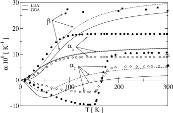
Figure 2: Linear thermal expansion for hcp Ti at ambient pressure. The solid lines are the theoretical calculation using GGA and the dashed line is from an LDA calculation. The filled circles are the experimental data of Nizhankovskii $et$ $al$ Misha . The filled squares are the experimental volume expansion coefficient of Mal’ko $et$ $al$ Malko . The filled and empty triangle are the experimental data of $\alpha_{a}$ and $\alpha_{c}$ respectively of Pawar $et$ $al$ Ram . The empty circles are the experimental data of Nizhankovskii $et$ $al$ scaled to give a volume expansion coefficient in agreement with Ref.Malko, .

The fact that both the measured and calculated thermal expansion coefficients along the c-axis of Ti are negative at low temperatures strongly suggests the uniqueness of elemental Ti among transition metals, although the absolute value of the measures low temperature expansion coefficient is still somewhat uncertain. The measured data of Ref. Misha, (filled circles) have in Fig. 2 been scaled (open circles) to reproduce room temperature values of $\beta$, $\alpha_{a}$ and $\alpha_{c}$, and it is found that these scaled values compare better with our theory (Fig. 2). Although a slight calibration error in Ref. Misha, can not be excluded, there is good reason to view the negative value of $\alpha_{c}$ at low temperatures as a true materials property of $\alpha$-Ti.

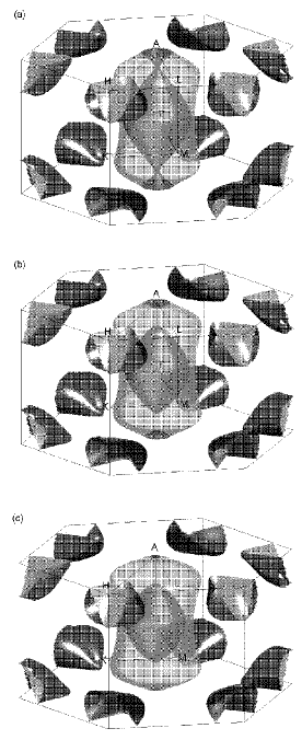
Figure 3: Calculated Fermi surface of hcp Ti at T=0 equilibrium volume for three different lattice constants c, at $c=0.988c_{0}$ (a), at $c=c_{0}$ (b) and at $c=1.012c_{0}$ (c). Here $c_{0}$ corresponds to the (T=0) equilibrium lattice constant.

As we will show below the microscopic origin of the negative thermal expansion for $\alpha_{c}$ of Ti is due to the closeness to a saddle point van Hoove singularity of the electronic structure. To illustrate this singularity we proceed with an analysis of the Fermi surface. In order to do this we show in Fig. 3 the calculated Fermi surface at the equilibrium volume for three different values of the out-of-plane lattice constant, c. The figure shows that as the c lattice constant decreases the inner ellipsoidal surface at the $\Gamma$-point and the Fermi surface centered at the $A$-point, become connected along the $\Gamma A$ line. The electronic structure as revealed by the Fermi surface shown in Fig.3 thus demonstrates the presence of a saddle point Van Hove singularity, which is associated with a singular contribution to the density of states at the Fermi level $N(E_{F}),$ $\delta N\left(E_{F}\right)\sim-\sqrt{E_{F}-E_{c1}}\theta(E_{F}-E_{c1})$ , where $\theta(x)$ fulfills: $\theta(x>0)=1$, $\theta(x<0)=0$ and $E_{c1}$ is the critical point energy Misha ; Antropov . The energy difference between $E_{F}$ and the energy of the critical saddle point, at the theoretical equilibrium volume and a c=$c_{0}$, has been calculated to be $E_{F}-E_{c1}\sim 44$ meV. Another critical point, associated with the appearance of a new ellipsoid around the $K$ symmetry point (not shown in Fig. 3 ) has been found in the calculations, giving rise to the singular contribution $\delta N(E_{F})\sim\sqrt{E_{c2}-E_{F}}\theta(E_{c2}-E_{F})$ to $N(E_{F})$. However since $E_{c2}-E_{F}\sim 142$ meV and $|\partial(E_{c2}-E_{F})/\partial\epsilon|\ll|\partial(E_{F}-E_{c1})/\partial\epsilon|$, it is clear that the saddle-point topological transition, at $E_{c1}$, gives rise to the strongest singular contribution to $N(E_{F})$.

By calculating the derivatives of $N(E_{F})$ with respect to the two different types of strains we have found that $\partial N(E_{F})/\partial\epsilon_{v}\sim 0.75$ eV^-1 and $\partial N(E_{F})/\partial\epsilon_{c}\sim-0.77$ eV^-1. Since the singularities in $N(E_{F})$ influence the elastic moduli, thus effecting the Debye temperature KNT , it is natural to attribute the main reason for the anisotropic thermal expansion in $\alpha-$titanium to the saddle-point Van Hove singularity near the Fermi level.

Acknowledgments We are grateful to the Strategic Foundation for Research (SSF), the Swedish Research Council (VR), the Swedish National Supercomputer Center (NSC), UPMAX and to the Göran Gustafsson foundation, for support. MIK acknowledges a support from Stichting voor Fundamenteel Onderzoek der Materie (FOM), the Netherlands. Valuable discussions with Prof. U. Jansson are acknowledged.

References

- (1) W. A. Harrison, Electronic Structure and the Properties of Solids (W.H.Freeman and Company, San Francisco, 1980).
- (2) With the exception of the complex structure of Mn at low temperatures.
- (3) H. L. Skriver, Phys. Rev. B 31, 1909 (1985).
- (4) V. L. Moruzzi, J. F. Janak, & K. Schwarz, Phys. Rev. B 37, 790 (1988).
- (5) V. I. Nizhankovskii, M. I. Katsnelson, G. V. Peschanskikh, & A. V. Trefilov, Pis’ma ZhETF 59, 693 (1994).
- (6) W. Hume-Rothery, The Metallic State (Oxford Univ. Press, 1931)
- (7) N. F. Mott, & H. Jones, The Theory of the Properties of Metals and Alloys (Oxford Univ. Press, 1936).
- (8) M. I. Katsnelson, I.I. Naumov, I.I. & A. V. Trefilov, Phase Transitions 49, 143 (1994).
- (9) I. M. Lifshitz, Sov. Phys. JETP 11, 1130 (1960).
- (10) V. G. Vaks et al., J. Phys.: Condens. Matter 1, 5319 (1989).
- (11) V. G. Vaks et al. J. Phys.: Condens. Matter 3 1409 (1991).
- (12) V. P. Antropov et. al., Phys. Lett. A 130, 155 (1988).
- (13) R. W. Munn, The Thermal Expansion of Axial Metals, Advances in physics, 18 (1969).
- (14) The first principles calculations were done with the VASP code vasp . Convergence in sampling of the Brillouin zone was obtained at 20480 k-points (for elastic constants) and 486 k-point (for phonon calculations). The calculations employed both the local density approximation (LDA) and the general gradient approximation (GGA). The phonon density of states were calculated using a k-point mesh with a 0.05 THz smearing. The calculations have been performed for 15 different volume strains in the range 0 , and at each volume strain for three different tetragonal strains , where is the tetragonal strain corresponding to the minimum static lattice energy at a given volume strain, . In the VASP calculations a cut-off of 302 eV was used. To each eigenvalue a Gaussian smearing of 0.2 eV was applied to speed up the convergence of the calculation.
- (15) G. Kresse & J. Furthmuller, Phys. Rev. B 54, 11169 (1996).
- (16) D. C. Wallace, Thermodynamics of Crystals ( Wiley, New York, 1972 ).
- (17) G. K. Straub, J. B. Aidun, J. M. Wills, C. R. SanchezCastro, & D. C. Wallace, Phys. Rev. B 50, 5055 (1994).
- (18) Yu. N. Gornostyrev et al, Scripta Metal. 56, 81 (2007)
- (19) P. Souvatzis, A. Delin, & O. Eriksson, Phys. Rev. B 73, 054110 (2006).
- (20) A. Sommerfeld & N. H. Frank, Rev. Mod. Phys. 3, 1 (1931) .
- (21) D. R. Trinkle et. al., Phys. Rev. B 73, 94123 (2006).
- (22) C. Stassis, D. Arch, B. N. Harmon & N. Wakabayashi, Phys. Rev. B 19, 181 (1979).
- (23) D. Alfé, The Phon-software together with a description of the program can be found at: http://chianti.geol.ucl.ac.uk/ dario/ .
- (24) P. I. Mal’ko, D. S. Arensburger, V. S. Pugin, V. F. Nemchenko, & S. N. L’Vov, Powder Metallurgy and Metal Ceramics, 9, 642 ( 1970).
- (25) R.R Pawar, and V.T. Deshpande, Acta Crystallogr. A 24, 316 (1968).