The Symmetric Tensor Lichnerowicz Algebra

The Symmetric Tensor Lichnerowicz Algebra
and a Novel Associative Fourier–Jacobi Algebra

Karl HALLOWELL and Andrew WALDRON

K. Hallowell and A. Waldron

Department of Mathematics, University of California, Davis CA 95616, USA

hallowell@math.ucdavis.edu, wally@math.ucdavis.edu

Received July 21, 2007; Published online September 13, 2007

Lichnerowicz’s algebra of differential geometric operators acting on symmetric tensors can be obtained from generalized geodesic motion of an observer carrying a complex tangent vector. This relation is based upon quantizing the classical evolution equations, and identifying wavefunctions with sections of the symmetric tensor bundle and Noether charges with geometric operators. In general curved spaces these operators obey a deformation of the Fourier–Jacobi Lie algebra of $sp(2,{\mathbb{R}})$. These results have already been generalized by the authors to arbitrary tensor and spinor bundles using supersymmetric quantum mechanical models and have also been applied to the theory of higher spin particles. These Proceedings review these results in their simplest, symmetric tensor setting. New results on a novel and extremely useful reformulation of the rank 2 deformation of the Fourier–Jacobi Lie algebra in terms of an associative algebra are also presented. This new algebra was originally motivated by studies of operator orderings in enveloping algebras. It provides a new method that is superior in many respects to common techniques such as Weyl or normal ordering.

symmetric tensors; Fourier–Jacobi algebras; higher spins; operator orderings

51P05; 53Z05; 53B21; 70H33; 81R99; 81S10

1 Introduction

The study of geometry using first quantized particle models has a long history. Notable examples are the study of Pontryagin classes and Morse theory in terms of ${\cal N}=1$ and ${\cal N}=2$ supersymmetric quantum mechanical models [2, 3]. The supercharges of those models correspond to Dirac, and exterior derivative and codifferential operators acting on spinors and forms, respectively. The model we concentrate on here describes gradient and divergence operators acting on symmetric tensors and therefore involves no supersymmetries at all. Hence, even though the symmetries of this model are analogous to supersymmetries, no knowledge of superalgebras is required to read these Proceedings. All the above models fit into a very general class of orthosymplectic spinning particle theories studied in detail by the authors in [4]. Spinors, differential forms, multiforms [5, 6, 7, 8, 9] and symmetric tensors [10, 11] are all fitted into a single framework in that work. Here we focus on the symmetric tensor case, both for its simplicity, and because we want to present new results on the symmetric tensor Lichnerowicz algebra developed in [11].

The underlying classical system is geodesic motion on a Riemannian manifold along with parallel transport of a complex tangent vector. This is described by a pair of ordinary differential equations to which we add further curvature couplings designed to maximize the set of constants of the motion. Of particular interest are symmetries interchanging the vector tangent to the manifold with the tangent vector to the geodesic. These are analogous to supersymmetries and correspond to gradient and divergence operators. This correspondence is achieved by quantizing the model. The complex tangent vector describes spinning degrees of freedom so that wavefunctions are sections of the symmetric tensor bundle. The Noether charges of the theory become operators on these sections. In particular, the Hamiltonian is a curvature modified Laplace operator. In fact, it is precisely the wave operator acting on symmetric tensors introduced some time ago by Lichnerowicz [10] on the basis of its algebraic properties on symmetric spaces [11]. Moreover, the set of all Noether charges obey a deformation of the Fourier–Jacobi Lie algebra $sp(2,{\mathbb{R}})^{J}$. The classical model is described in Section 2, while its quantization and relation to geometry are given in Section 3.

Applications, such as higher spin theories [11, 15], call for expressions in the universal enveloping algebra ${\cal U}(sp(2,{\mathbb{R}})^{J})$ involving arbitrarily high powers of the generators. Manipulating these expressions requires a standard ordering, oft used examples being Weyl ordering (averaging over operator orderings) or normal ordering (based on a choice of polarization such that certain operators are moved preferentially to the right, say). In a study of partially massless higher spins [16], we found a new operator ordering scheme to be particularly advantageous [11]. The key idea is to rewrite generators of the $sp(2,{\mathbb{R}})$ subalgebra, wherever possible, as powers of Cartan elements or the quadratic Casimir operator. Immediately, this scheme runs into a difficulty, namely that the remaining $sp(2,{\mathbb{R}})^{J}$ generators do not have a simple commutation relation with the quadratic $sp(2,{\mathbb{R}})$ Casimir. This problem is solved by a trick: we introduce a certain square root of the quadratic Casimir whose rôle is to measure how far states are from being highest weight. Then we use this square root operator to construct modified versions of the remaining $sp(2,{\mathbb{R}})^{J}$ generators. Instead of a simple Lie algebra, we then obtain an elegant associative algebra, which we denote $\widetilde{\,\cal U\,}\!(sp(2,{\mathbb{R}}))$, with relations allowing elements to be easily reordered. This algebra is described and derived in detail in Section 4. The final Section discusses applications and our conclusions.

2 The classical model

Let $(M,g_{\mu\nu})$ be an $n$-dimensional (pseudo-)Riemannian manifold with an orthonormal frame $e^{m}$ so that $ds^{2}=dx^{\mu}g_{\mu\nu}dx^{\nu}=e^{m}\eta_{mn}e^{n}$. We consider the motion of an ant $x^{\mu}(t)$ – as depicted in Fig. 1 – who carries a complex vector $z^{m}(t)$ (expressed relative to the orthonormal frame) tangent to $M$. (In physics nomenclature, $z^{m}$ is referred to as commuting spinning degrees of freedom.) The Levi-Civita connection will be denoted by $\nabla$. The ant determines its path and in which direction to hold the complex vector by the system of generalized geodesic ODEs

$$\frac{\nabla\dot{x}^{\mu}}{dt}=\dot{x}^{\nu}R^{\mu}{}_{\nu}{}^{m}{}_{n}z^{*}_{m}z^{n}+\nabla^{\mu}\!R^{m}{}_{n}{}^{r}{}_{s}\,z^{*}_{m}z^{n}z^{*}_{r}z^{s},$$

$$\frac{\nabla z^{m}}{dt}=iR^{m}{}_{n}{}^{r}{}_{s}\,z^{n}z_{r}^{*}z^{s}.$$ (1)

The non-linear couplings to the curvature tensor on the right hand side of these equations have been carefully chosen to maximize the set of constants of the motion. They may obtained by extremizing a generalized energy integral

$$S=\int dt\left\{\frac{1}{2}\dot{x}^{\mu}g_{\mu\nu}\dot{x}^{\nu}+iz_{m}^{*}\frac{\nabla z^{m}}{dt}+\frac{1}{2}R^{m}{}_{n}{}^{r}{}_{s}\,z^{*}_{m}z^{n}z^{*}_{r}z^{s}\right\}.$$ (2)

To study constants of the motion, we look for symmetries of this action principle. The most obvious of these are translations of $t\rightarrow t+\xi$ along the parameterized path traversed by our ant. Infinitesimally this yields the invariance

$$\delta x^{\mu}=\xi\dot{x}^{\mu},\qquad\delta z^{m}=\xi\dot{z}^{m}.$$

Less trivial, are symplectic transformations of $(z^{m},z_{m}^{*})$,

$$\delta z^{m}=-\alpha z^{m}+\beta z^{*m},\qquad\delta z^{*m}=\gamma z^{m}+\alpha z^{*m}.$$

The parameters $(\alpha,\beta,\gamma)$ are real and correspond to the Lie algebra $sp(2,{\mathbb{R}})$. The astute reader will observe that the symmetry transformation of $z^{*m}$ is not the complex conjugate of $z^{m}$. Nonetheless, treating $z^{m}$ and $z^{*m}$ as independent variables, the above $sp(2,{\mathbb{R}})$ transformations do leave the action invariant. This is in fact sufficient to ensure existence of corresponding constants of the motion and Noether charges. In the quantum theory, these charges will play an important geometric rôle.

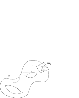
Figure 1: An ant laden with a complex tangent vector.

The most interesting symmetries of the model interchange the complex tangent vector $z^{m}$ with the tangent vector $\dot{x}^{\mu}$ to the ant’s path

$$\delta x^{\mu}=i(z^{*\mu}\varepsilon-z^{\mu}\varepsilon^{*}),\qquad{\cal D}z^{\mu}=\dot{x}^{\mu}\varepsilon.$$ (3)

Here, ${\cal D}$ is the covariant variation and is defined by ${\cal D}v^{\mu}\equiv\delta v^{\mu}+\Gamma^{\mu}_{\rho\sigma}\delta x^{\rho}v^{\sigma}$ where $\Gamma$ denotes the Christoffel symbols. It saves one from having to vary covariantly constant quantities.

The transformations (3) are not an exact symmetry for an arbitrary Riemannian manifold. In fact, the action (2) is invariant only when the locally symmetric space condition

$$\nabla_{\kappa}R_{\mu\nu\rho\sigma}=0,$$ (4)

holds. Or in other words, the Riemann tensor is covariantly constant. Constant curvature spaces provide an, but by no means the only, example of such a manifold.

To compute constants of the motion we work in a first order formulation

$$\dot{x}^{\mu}=\pi^{\mu}.$$

This and the evolution equations (1) also follow from an action principle

$$S^{(1)}=\int dt\left\{p_{\mu}\dot{x}^{\mu}+iz^{*}_{m}\dot{z}^{m}-\frac{1}{2}\pi_{\mu}g^{\mu\nu}\pi_{\nu}+\frac{1}{2}R^{m}{}_{n}{}^{r}{}_{s}\,z^{*}_{m}z^{n}z^{*}_{r}z^{s}\right\},$$ (5)

where the covariant and canonical momenta $\pi_{\mu}$ and $p_{\mu}$ are related by

$$\pi_{\mu}=p_{\mu}-i\omega_{\mu}{}^{m}{}_{n}z_{m}^{*}z^{n}.$$

Here the spin connection is determined by requiring covariant constancy of the orthonormal frame $\nabla_{\rho}e_{\mu}{}^{m}=\partial_{\rho}e_{\mu}{}^{m}-\Gamma_{\rho\mu}^{\nu}e_{\nu}{}^{m}+\omega_{\rho}{}^{m}{}_{n}e_{\mu}{}^{n}=0$.

From the first order action (5) we immediately read off the contact one-form $p_{\mu}dx^{\mu}+iz_{m}^{*}dz^{m}$ which is already in Darboux coordinates, so Poisson brackets follow immediately

$$\{p_{\mu},x^{\nu}\}_{\rm PB}=\delta_{\mu}^{\nu},\qquad\{z^{m},z^{*}_{n}\}_{\rm PB}=i\delta_{n}^{m}.$$

The Noether charges for the symmetries of the model can now be computed

$$H=\frac{1}{2}\pi_{\mu}g^{\mu\nu}\pi_{\nu}-\frac{1}{2}R^{m}{}_{n}{}^{r}{}_{s}\,z^{*}_{m}z^{n}z^{*}_{r}z^{s},$$

$$f=\left(\begin{array}[]{cc}z^{*}_{m}z^{*m}&z^{*}_{m}z^{m}\vspace{1mm}\\ z^{*}_{m}z^{m}&z_{m}z^{m}\end{array}\right),\qquad v=\ \left(\begin{array}[]{c}iz^{*\mu}\pi_{\mu}\vspace{1mm}\\ iz^{\mu}\pi_{\mu}\end{array}\right).$$ (10)

The first of these is the Hamiltonian. We have arranged the symplectic symmetry charges in a symmetric matrix $f$ using the isomorphism between the symplectic Lie algebra and symmetric matrices. The remaining charges appear as a column vector $v$ since they in fact form a doublet representation of $sp(2,{\mathbb{R}})$. It is important to remember that this latter pair of charges are constants of the motion for locally symmetric spaces only.

3 Quantization and geometry

Quantization proceeds along usual lines replacing the Poisson brackets by quantum commutators $[p,x]=-i\hbar$ and $[z,z^{*}]=\hbar$. We set $\hbar=1$ in what follows and represent the canonical momentum as a derivative acting on wavefunctions $\psi(x^{\mu})$

$$p_{\mu}=\frac{1}{i}\frac{\partial}{\partial x^{\mu}}.$$

The spinning degrees of freedom become oscillators acting on a Fock space. Rather than using the standard notation $z^{m}=a^{m}$ annihilating a Fock vacuum $a^{m}|0\rangle$, we represent $|0\rangle=1$ and to preempt their geometric interpretation, set

$$z^{*\mu}=dx^{\mu},\qquad z_{\mu}=\frac{\partial}{\partial(dx^{\mu})}.$$

Therefore, wavefunctions become

$$\Psi=\sum_{s=0}^{\infty}\psi_{\mu_{1}\ldots\mu_{s}}(x)dx^{\mu_{1}}\cdots dx^{\mu_{s}},$$

or in words – sections of the symmetric tensor bundle $SM$ over $M$. Therefore, we can now start relating quantum mechanical operations to differential geometry ones on symmetric tensors. Firstly, the quantum mechanical inner product yields the natural inner product for symmetric tensors

$$\langle\Phi|\Psi\rangle=\int_{M}\sum_{s=0}^{\infty}s!\sqrt{g}\,\phi^{\mu_{1}\ldots\mu_{s}}\psi_{\mu_{1}\ldots\mu_{s}}.$$

Furthermore, the covariant momentum corresponds to the covariant derivative $i\pi_{\mu}\Psi=\nabla_{\mu}\Psi$ (it is necessary to contract the open index $\mu$ with $dx^{\mu}$ for this to hold true for subsequent applications of $\pi_{\mu}$).

Next we turn to the symplectic symmetries $f$ in (10). We call the off-diagonal charge

$${\bf N}=dx^{\mu}\frac{\partial}{\partial(dx^{\mu})},$$

which simply counts the number of indices of a symmetric tensor

$${\bf N}\;\psi_{\mu_{1}\ldots\mu_{s}}dx^{\mu_{1}}\cdots dx^{\mu_{s}}=s\,\psi_{\mu_{1}\ldots\mu_{s}}dx^{\mu_{1}}\cdots dx^{\mu_{s}}.$$

We call the diagonal charges

$${\bf g}=dx^{\mu}g_{\mu\nu}dx^{\nu},\qquad{\bf tr}=\frac{\partial}{\partial(dx^{\mu})}\,g^{\mu\nu}\frac{\partial}{\partial(dx^{\nu})},$$

as they produce new symmetric tensors by either multiplying by the metric tensor and symmetrizing, or tracing a pair of indices

$${\bf g}\ \psi_{\mu_{1}\ldots\mu_{s}}dx^{\mu_{1}}\cdots dx^{\mu_{s}}=g_{(\mu_{1}\mu_{2}}\psi_{\mu_{3}\ldots\mu_{s+2})}dx^{\mu_{1}}\cdots dx^{\mu_{s+2}},$$

$${\bf tr}\ \psi_{\mu_{1}\ldots\mu_{s}}dx^{\mu_{1}}\cdots dx^{\mu_{s}}=s(s-1)\psi^{\mu}{}_{\mu\mu_{1}\ldots\mu_{s-2}}dx^{\mu_{1}}\cdots dx^{\mu_{s-2}}.$$

These three operators obey the $sp(2,{\mathbb{R}})$ Lie algebra

$$[{\bf N},{\bf tr}]=-2\,{\bf tr},\qquad[{\bf N},{\bf g}]=2\,{\bf g},\qquad[{\bf tr},{\bf g}]=4\,{\bf N}+2n.$$

We call its quadratic Casimir

$${\bf c}={\bf g}\,{\bf tr}-{\bf N}({\bf N}+n-2).$$

Trace-free symmetric tensors with a definite number of indices, $({\bf N}-s)\Psi=0={\bf tr}\Psi$, are the highest weight vectors for unitary discrete series representations of this $sp(2,{\mathbb{R}})$ algebra.

The Noether charges $v$ in (10) are linear in momenta and therefore covariant derivatives, when acting on wavefunctions. We call them the gradient and divergence,

$${\bf grad}=dx^{\mu}\nabla_{\mu},\qquad{\bf div}=\frac{\partial}{\partial(dx^{\mu})}\nabla^{\mu},$$

because they are natural generalizations to symmetric tensors of the exterior derivative and codifferential for differential forms. To be sure

$${\bf grad}\,\psi_{\mu_{1}\ldots\mu_{s}}dx^{\mu_{1}}\cdots dx^{\mu_{s}}=\nabla_{(\mu_{1}}\psi_{\mu_{2}\ldots\mu_{s+1})}dx^{\mu_{1}}\cdots dx^{\mu_{s+1}},$$

$${\bf div}\,\psi_{\mu_{1}\ldots\mu_{s}}dx^{\mu_{1}}\cdots dx^{\mu_{s}}=s\nabla^{\mu}\psi_{\mu\mu_{1}\ldots\mu_{s-1}}dx^{\mu_{1}}\cdots dx^{\mu_{s-1}}.$$

This pair of operators forms the defining representation of $sp(2,{\mathbb{R}})$

$$[{\bf N},{\bf grad}]={\bf grad},\qquad[{\bf N},{\bf div}]=-{\bf div},\qquad[{\bf tr},{\bf grad}]=2\,{\bf div},\qquad[{\bf div},{\bf g}]=2\,{\bf grad}.$$

It remains to commute the operators ${\bf div}$ and ${\bf grad}$. The result is

$$[{\bf div},{\bf grad}]=\Delta-R^{\#\#},$$ (11)

where $\Delta=\nabla^{\mu}\nabla_{\mu}$ is the Bochner Laplacian and

$$R^{\#\#}\equiv R_{\mu}{}^{\nu}{}_{\rho}{}^{\sigma}dx^{\mu}\frac{\partial}{\partial(dx^{\nu})}dx^{\rho}\frac{\partial}{\partial(dx^{\sigma})}.$$

This relation is closely analogous to that for the exterior derivative and codifferential $\{d,\delta\}=\Delta_{F}$ where $\Delta_{F}$ is the form-Laplacian. Here, since we are dealing with symmetric tensors, the anticommutator is replaced by a commutator. A shrewd reader might sense that the second order operator on the right hand side of (11) should be related to the quantum mechanical Hamiltonian operator. This is indeed the case; calling $\square=\Delta+R^{\#\#}$, we have

$$[{\bf div},{\bf grad}]=\square-2R^{\#\#},$$

where $\square=-2H$ so long as an appropriate operator ordering is chosen for the Hamiltonian (a full account is given in [4]). On any manifold

$$[\square,{\bf g}]=[\square,{\bf N}]=[\square,{\bf tr}]=0.$$

Moreover, whenever the symmetric space condition (4) holds, the operator $\square$ is central

$$[\square,{\bf div}]=[\square,{\bf grad}]=0.$$

In fact, $\square$ is precisely the wave operator introduced quite some time ago by Lichnerowicz on the basis of its special algebra with gradient and divergence operators [10]. Finally, in the special case of constant curvature manifolds, choosing units in which the scalar curvature $R=-n(n-1)$, the curvature operator $R^{\#\#}$ equals the $sp(2,{\mathbb{R}})$ Casimir so that

$$[{\bf div},{\bf grad}]=\square-2{\bf c}.$$ (12)

If we include a further operator ${\bf ord}$ whose rôle is to count derivatives

$$[{\bf ord},{\bf g}]=[{\bf ord},{\bf N}]=[{\bf ord},{\bf tr}]=0,$$

$$[{\bf ord},{\bf grad}]={\bf grad},\qquad[{\bf ord},{\bf div}]={\bf div},\qquad[{\bf ord},\square]=2\square,$$

then, $\{{\bf ord},{\bf g},{\bf N},{\bf tr},{\bf grad},{\bf div},\square\}$ form a maximal parabolic subgroup of $sp(4,{\mathbb{R}})$ up to the rank 2 deformation by the $sp(2,{\mathbb{R}})$ Casimir in (12). On flat manifolds $M$, the operators $\{{\bf g},{\bf N},{\bf tr}$, ${\bf grad},{\bf div},\square\}$ obey the Fourier–Jacobi Lie algebra of $sp(2,{\mathbb{R}})$. In the next Section, we present a novel reformulation of its universal enveloping algebra based on introducing a certain square root of the Casimir operator ${\bf c}$.

4 The Fourier–Jacobi algebra

Figure 2: The root diagram for the Fourier–Jacobi Lie algebra.

Let us first collect together the deformed Fourier–Jacobi Lie algebra built from geometric operators on constant curvature spaces

$[{\bf tr},{\bf g}]=4\,{\bf N}+2n,$

$\!\!\!\!\!\![{\bf N},{\bf tr}]=-2\,{\bf tr},\qquad\quad\ \ \ [{\bf N},{\bf g}]=2\,{\bf g},$

$[{\bf N},{\bf grad}]={\bf grad},\qquad\qquad[{\bf N},{\bf div}]=-{\bf div},$

$[{\bf tr},{\bf grad}]=2\,{\bf div},\qquad\qquad[{\bf div},{\bf g}]=2\,{\bf grad},$

$[{\bf div},{\bf grad}]=\square-2{\bf c}.$

Its root diagram is given in Fig. 2. From now on we compute in the explicit realization given by its action on sections of the symmetric tensor bundle. Therefore we are working with linear operators, so any algebra we find is automatically consistent and associative.

To start with we analyze the $sp(2,{\mathbb{R}})$ Lie algebra built from $\{\bf g,N,tr\}$. Unitary discrete series representations with respect to the adjoint involution ${\bf tr}^{\dagger}={\bf g}$, ${\bf N^{\dagger}=N}$ are built from highest weights $\Phi$ such that

$${\bf N}\,\Phi=s\Phi,\qquad{\bf tr}\,\Phi=0.$$

The highest weight module is spanned by

$$\{\Phi,{\bf g}\,\Phi,{\bf g}^{2}\Phi,\ldots\}.$$

We can characterize this representation by the eigenvalue $s$ of ${\bf N}$ acting on the highest weight, or alternatively by the eigenvalue $-s(s+n-2)$ of the Casimir ${\bf c}$ acting on any state in the module.

Conversely, given a eigenstate $\Psi$ of ${\bf N}$ and ${\bf c}$, we can determine which discrete series representation it belongs to by repeatedly applying the trace operator

$${\bf tr}^{k}\Psi\neq 0={\bf tr}^{k+1}\Psi,$$

which implies that $\Psi$ can be expressed in terms of a highest weight vector as $\Psi={\bf g}^{k}\,\Phi$. Our key observation is that it is highly advantageous to introduce the linear operator $\kappa$ whose eigenvalue acting on $\Psi$ is the depth $k$, namely

$${\mbox{\boldmath$\kappa$}}\equiv\frac{{\cal N-C}-1}{2},$$ (13)

where

$${\cal N}\equiv{\bf N}+\frac{n}{2},\qquad{\cal C}\equiv\sqrt{\left(\frac{n-2}{2}\right)^{2}-{\bf c}}.$$

In other words, $\kappa$ measures how far the symmetric tensor $\Psi$ is from being trace-free. The operator $4\,{\cal N}$ is simply the right hand side of the ${\bf tr}$, ${\bf g}$ commutator. More important is the square root of the Casimir ${\cal C}$ which acts on the highest weight $\Phi$ as

$${\cal C}\,\Phi=\left[s+\frac{n-2}{2}\right]\Phi,$$

which explains equation (13).

Our claim is that for many applications involving high powers of the operators ${\bf g}$, ${\bf N}$ and ${\bf tr}$, rather than normal or Weyl orderings it is far more expeditious to work with functions of ${\cal N}$, ${\cal C}$ (up to perhaps an overall power of ${\bf g}$ or ${\bf tr}$). By way of translation, we note that a normal ordered product of ${\bf g}$ and ${\bf tr}$ can be expressed as Pochhammer functions of $({\cal N,C})$ :

$${\bf g}\,{\bf tr}=({\cal N-C}-1)({\cal N+C}-1),\qquad\Rightarrow$$

$$:({\bf g\,tr})^{m}:\equiv{\bf g}^{m}{\bf tr}^{m}=\frac{1}{4^{m}}\ \left(\frac{{\cal C-N}+1}{2}\right)_{m}\left(\frac{{\cal C+N}-1}{2}\right)_{m}.$$

This claim has little significance until we introduce the doublet $({\bf grad,div})$. Indeed, since the Casimir ${\bf c}$ has a rather unpleasant commutation relation with either of these operators, computing in terms of $({\cal N,C})$ may seem unwise. In fact this is not the case once one appropriately modifies the divergence and gradient operators.

To motivate the claim we return to symmetric tensors. Suppose $\varphi_{\mu_{1}\ldots\mu_{s}}$ is trace-free, then its gradient $\nabla_{(\mu_{1}}\varphi_{\mu_{2}\ldots\mu_{s+1})}$ is in general not trace free (unless the divergence of $\varphi$ happens to vanish). Since we would like to work with states diagonalizing both ${\bf c}$ and ${\bf N}$, it is propitious to replace the regular gradient with its trace-free counterpart

$$\nabla_{(\mu_{1}}\varphi_{\mu_{2}\ldots\mu_{s+1})}-\frac{s}{2s+n-2}\ g_{(\mu_{1}\mu_{2}}\nabla^{\mu}\varphi_{\mu_{3}\ldots\mu_{s+1})\mu}.$$

We denote this operator by $\widetilde{\bf grad}$. Having introduced ${\cal C}$ and ${\cal N}$, it has the simple expression

$$\widetilde{\bf grad}\equiv{\bf grad}-{\bf g}\,{\bf div}\,\frac{1}{{\cal N+C}-1},$$ (14)

which we take to be its definition acting on any section of the symmetric tensor bundle. It is important to note that although this operator maps trace-free tensors to trace-free tensors, it is designed to maintain how far a more general tensor is from being trace-free. Therefore it does not project arbitrary tensors to trace-free ones. We also introduce a similar definition for a trace-free divergence following from the quantum mechanical adjoint ${\bf grad}^{\dagger}=-{\bf div}$

$$\widetilde{\bf div}\equiv\ {\bf div}-\frac{1}{{\cal N+C}-1}\,{\bf grad}\,{\bf tr}.$$ (15)

Note also that the linear operator ${{\cal N+C}-1}$ is indeed invertible since its spectrum is $2s+2k+n-2$ on eigenstates ${\bf g}^{k}\Phi$ (these expressions also make sense in dimensions $n=1,2$ thanks to the operators ${\bf div}$ and ${\bf grad}\,{\bf tr}$).

The beauty of the operators $({\bf\widetilde{div},\widetilde{grad}})$ is that they commute with the depth operator $\kappa$. This implies

$${\cal N}\,\widetilde{\bf div}=\widetilde{\bf div}\,({\cal N}-1),\qquad {\cal N}\,\widetilde{\bf grad}=\widetilde{\bf grad}\,({\cal N}+1),$$

$${\cal C}\,\widetilde{\bf div}=\widetilde{\bf div}\,({\cal C}-1),\qquad {\cal C}\,\widetilde{\bf grad}=\widetilde{\bf grad}\,({\cal C}+1).$$

Moreover, an easy computation using the definitions (14) and (15) shows that the ordering of gradient and metric operators can be interchanged at the cost of only a rational function of $({\cal C,N})$

$$\widetilde{\bf grad}\,{\bf g}={\bf g}\,\widetilde{\bf grad}\,\frac{{\cal N+C}-1}{{\cal N+C}+1},\qquad{\bf tr}\,\widetilde{\bf div}=\frac{{\cal N+C}-1}{{\cal N+C}+1}\,\widetilde{\bf div}\,{\bf tr}.$$

These relations allow us to invert equations (14) and (15)

$${\bf grad}=\frac{1}{2}\,\frac{{\cal N+C}-3}{{\cal C}-1}\,\widetilde{\bf grad}+\frac{1}{2\cal C}\,\frac{{\cal N+C}-3}{{\cal N+C}-1}\,{\bf g}\,\widetilde{\bf div},$$

$${\bf div}=\frac{1}{2}\,\widetilde{\bf div}\ \frac{{\cal N+C}-3}{{\cal C}-1}+\frac{1}{2}\,\widetilde{\bf grad}\,{\bf tr}\,\frac{{\cal N+C}-3}{{\cal C(N+C}-1)}.$$

In turn we can now compute relations for reordering the gradient and trace operators

$${\bf tr}\,\widetilde{\bf grad}=\frac{({\cal N+C}+1)({\cal N+C}-3)}{({\cal N+C}-1)^{2}}\,\widetilde{\bf grad}\ {\bf tr},$$

$$\widetilde{\bf div}\,{\bf g}={\bf g}\,\widetilde{\bf div}\,\frac{({\cal N+C}+1)({\cal N+C}-3)}{({\cal N+C}-1)^{2}}.$$

The final relation we need is for $\widetilde{\bf div}$ and $\widetilde{\bf grad}$. After some computations we find

$$\widetilde{\bf div}\,\widetilde{\bf grad}=\frac{{\cal C}^{2}({\cal N+C}+1)({\cal N+C}-3)^{2}}{({\cal C}+1)({\cal C}-1)({\cal N+C}-1)^{3}}\,\widetilde{\bf grad}\,\widetilde{\bf div}$$

$$\phantom{\widetilde{\bf div}\,\widetilde{\bf grad}=}{}+\frac{2{\cal C}^{2}({\cal N+C}+1)}{({\cal C}+1)({\cal N+C}-1)^{2}}\left[\square+2\left({\cal C}+\frac{n}{2}-1\right)\left({\cal C}-\frac{n}{2}+1\right)\right].$$

This result is valid in constant curvature spaces. The term in square brackets equals $[\square-2{\bf c}]$ and will be modified accordingly upon departure from constant curvature.

${\cal C}\,{\cal N}={\cal N}\,{\cal C}$

${\bf tr}\,{\bf g}=({\cal N+C}+1)({\cal N-C}+1)$

${\bf g}\,{\bf tr}=({\cal N+C}-1)({\cal N-C}-1)$

${\cal N}\,{\bf tr}={\bf tr}\,({\cal N}-2)\qquad\qquad{\cal N}\,{\bf g}={\bf g}\,({\cal N}+2)$

${\cal C}\,{\bf tr}={\bf tr}\,{\cal C}\qquad\qquad{\cal C}\,{\bf g}={\bf g}\,{\cal C}$

${\cal N}\,\widetilde{\bf div}=\widetilde{\bf div}\,({\cal N}-1)\qquad\qquad{\cal N}\,\widetilde{\bf grad}=\widetilde{\bf grad}\,({\cal N}+1)$

${\cal C}\,\widetilde{\bf div}=\widetilde{\bf div}\,({\cal C}-1)\qquad\qquad{\cal C}\,\widetilde{\bf grad}=\widetilde{\bf grad}\,({\cal C}+1)$

$\displaystyle\widetilde{\bf grad}\,{\bf g}={\bf g}\ \widetilde{\bf grad}\,\frac{{\cal N+C}-1}{{\cal N+C}+1}$     $\displaystyle{\bf tr}\,\widetilde{\bf div}=\frac{{\cal N+C}-1}{{\cal N+C}+1}\,\widetilde{\bf div}\ {\bf tr}\,\ \ \$

$\displaystyle{\bf tr}\,\widetilde{\bf grad}=\frac{({\cal N+C}+1)({\cal N+C}-3)}{({\cal N+C}-1)^{2}}\,\widetilde{\bf grad}\,{\bf tr}$

$\displaystyle\widetilde{\bf div}\,{\bf g}={\bf g}\,\widetilde{\bf div}\,\frac{({\cal N+C}+1)({\cal N+C}-3)}{({\cal N+C}-1)^{2}}$

$\displaystyle\widetilde{\bf div}\ \widetilde{\bf grad}=\frac{{\cal C}^{2}({\cal N+C}+1)({\cal N+C}-3)^{2}}{({\cal C}+1)({\cal C}-1)({\cal N+C}-1)^{3}}\ \widetilde{\bf grad}\ \widetilde{\bf div}\ \ \ \quad\qquad\qquad\quad\ \,$

$\displaystyle\phantom{\widetilde{\bf div}\ \widetilde{\bf grad}=}{}+\frac{2{\cal C}^{2}({\cal N+C}+1)}{({\cal C}+1)({\cal N+C}-1)^{2}}\left[\square+2\left({\cal C}+\frac{n}{2}-1\right)\left({\cal C}-\frac{n}{2}+1\right)\right]$

Figure 3: Defining relations for the $\widetilde{\,\cal U\,}\!(sp(2,{\mathbb{R}})^{J})$ algebra.

We denote the new algebra built from $\{{\bf g,{\cal N},tr,{\cal C},\widetilde{grad},\widetilde{div},\square}\}$ by $\widetilde{\,\cal U\,}\!(sp(2,{\mathbb{R}})^{J})$ and have collected together its defining relations in Fig. 3. As it is defined by linear operators acting on symmetric tensors, associativity is assured. An interesting, yet open, question is whether it can be defined on the universal enveloping algebra of $sp(2,{\mathbb{R}})^{J}$. Nonetheless, the explicit symmetric tensor representation guarantees its consistency and therefore we may study it and its representations as an abstract algebra in its own right.

5 Conclusions

We have presented a detailed study of symmetric tensors on curved manifolds. The key technology employed is the quantum mechanics of a bosonic spinning particle model. Also, many of our constructions were originally motivated by studies of higher spin quantum field theories [11]. The spinning particle model presented here is one of a general class of orthosymplectic spinning particle models that describe spinors, differential forms, multiforms, and indeed the most general tensor-spinor fields on a Riemannian manifold [4].

There are many applications and further research avenues. One simple question is that given the strong analogy between the theory of differential forms and the symmetric tensor one presented here, are there symmetric tensor analogs of de Rham cohomology? The answer is yes. Recall, for example, the Maxwell detour complex

$$\begin{array}[]{ccccccccccc}&&&d&&&&\delta&\\ 0&\longrightarrow&\Lambda^{0}M&\longrightarrow&\Lambda^{1}M&\rightarrow\cdots\!\ \!\ \cdots\rightarrow&\Lambda^{1}M&\longrightarrow&\Lambda^{0}M&\longrightarrow&0.\\ &&&&\hskip 1.9919pt|&\raisebox{1.16656pt}{\text@underline{\phantom{eeeseeyesyesyesyeseee}}}&\uparrow\\ &&&&&\delta d\end{array}$$ (20)

This is mathematical shorthand for Maxwell’s electromagnetism in curved backgrounds. The physics translation is to replace the sequence of antisymmetric tensor bundles $(\Lambda^{0}M,\,\Lambda^{1}M,\,\Lambda^{1}M$, $\Lambda^{0}M)$ by the words

$$\mbox{\it(gauge parameters, potentials, field equations, Bianchi identities)}.$$

Then the fact that (20) is a complex implies that Maxwell’s equations $\delta dA=0$ are gauge invariant because $\delta dd=0$, and subject to a Bianchi identity as $\delta\delta d=0$. An analogous complex exists for symmetric tensors although not in general backgrounds, for brevity we give the flat space result [13, 11]

$$\begin{array}[]{ccccccccccc}&&&{\bf grad}&&&&{\bf div}&\\ 0&\longrightarrow&SM&\longrightarrow&SM&\rightarrow\cdots\ \!\ \cdots\rightarrow&SM&\longrightarrow&SM&\longrightarrow&0,\\ &&&&\hskip 1.9919pt|&\raisebox{0.99594pt}{\text@underline{\phantom{eeyeseyesyesyesyesee}}}&\uparrow\\ &&&&&G\end{array}$$

where

$$G=\square-{\bf grad}\,{\bf div}+\frac{1}{2}\left({\bf grad}^{2}\,{\bf tr}+{\bf g}\,{\bf div}^{2}\right)-\frac{1}{2}{\bf g}\left(\square+\frac{1}{2}{\bf grad}\,{\bf div}\right){\bf tr}.$$

Notice that we have specified no grading on the symmetric tensor bundle $SM$. In fact the operator $G$ is the generating function for the equations of motion (and actions) for massless higher spins of arbitrary degree. A very fascinating question is whether such complexes exist for the most general orthosymplectic spinning particle models – preliminary studies suggest an affirmative answer [17].

Another interesting open question is the generality of the algebra $\widetilde{\,\cal U\,}(sp(2,{\mathbb{R}})^{J})$. For example, does there exist an algebra $\widetilde{\,\cal U\,}(osp(2p|Q)^{J})$ where $osp$ denotes the orthosymplectic superalgebra. Since the key idea is to include the square root of the Casimir operator in the algebra, higher rank generalizations ought involve the higher order Casimir operators. A positive answer to this question would be most welcome and is under investigation [18].

Acknowledgements

It is a pleasure to thank the organizers of the 2007 Midwest Geometry Conference, and especially Susanne Branson for a truly excellent meeting in honor of Tom Branson. We thank David Cherney, Stanley Deser, Rod Gover, Andrew Hodge, Greg Kuperberg, Eric Rains and Abrar Shaukat for discussions.

References

- [1]
- [2] Alvarez-Gaume L., Witten E., Gravitational anomalies, Nuclear Phys. B 234 (1984), 269–330.
- [3] Witten E., Supersymmetry and Morse theory, J. Differential Geom. 17 (1982), 661–692.
- [4] Hallowell K., Waldron A., Supersymmetric quantum mechanics and super-Lichnerowicz algebras, Comm. Math. Phys., to appear, hep-th/0702033.
-
[5]
Olver P.J., Differential hyperforms I, University of Minnesota, Report 82-101, 1982, 118 pages.
Olver P.J., Invariant theory and differential equations, in Invariant Theory, Editor S. Koh, Lecture Notes in Math., Vol. 1278, Springer-Verlag, Berlin, 1987, 62–80. -
[6]
Dubois-Violette M., Henneaux M.,
Generalized cohomology for irreducible tensor fields of mixed Young symmetry type,
Lett. Math. Phys. 49 (1999), 245–252, math.QA/9907135.
Dubois-Violette M., Henneaux M., Tensor fields of mixed Young symmetry type and complexes, Comm. Math. Phys. 226 (2002), 393–418, math.QA/0110088. - [7] Edgar S.B., Senovilla J.M.M., A weighted de Rham operator acting on arbitrary tensor fields and their local potentials, J. Geom. Phys. 56 (2006), 2153–2162.
-
[8]
Bekaert X., Boulanger N.,
Tensor gauge fields in arbitrary representations of . Duality and Poincaré lemma,
Comm. Math. Phys. 245 (2004), 27–67, hep-th/0208058.
Bekaert X., Boulanger N., On geometric equations and duality for free higher spins, Phys. Lett. B 561 (2003), 183–190, hep-th/0301243.
Bekaert X., Boulanger N., Tensor gauge fields in arbitrary representations of , Comm. Math. Phys. 271 (2007), 723–773, hep-th/0606198. -
[9]
de Medeiros P., Hull C.,
Geometric second order field equations for general tensor gauge fields,
JHEP 2003 (2003), no. 5, 019, 26 pages, hep-th/0303036.
de Medeiros P., Hull C., Exotic tensor gauge theory and duality, Comm. Math. Phys. 235 (2003), 255–273, hep-th/0208155. -
[10]
Lichnerowicz A.,
Propagateurs et commutateurs en relativité générale,
Inst. Hautes Études Sci. Publ. Math. (1961), no. 10, 56 pages.
Lichnerowicz A., Champs spinoriels et propagateurs en relativité générale, Bull. Soc. Math. France 92 (1964), 11–100. - [11] Hallowell K., Waldron A., Constant curvature algebras and higher spin action generating functions, Nuclear Phys. B 724 (2005), 453–486, hep-th/0505255.
-
[12]
Duval C., Lecomte P., Ovsienko V.,
Conformally equivariant quantization: existence and uniqueness,
Ann. Inst. Fourier (Grenoble) 49 (1999), 1999–2029, math.DG/9902032.
Duval C., Ovsienko V., Conformally equivariant quantum Hamiltonians, Selecta Math. (N.S.) 7 (2001), 291–320. - [13] Labastida J.M.F., Massless particles in arbitrary representations of the Lorentz group, Nuclear Phys. B 322 (1989), 185–209.
- [14] Vasiliev M.A., Equations of motion of interacting massless fields of all spins as a free differential algebra Phys. Lett. B 209 (1988), 491–497.
- [15] Bekaert X., Cnockaert S., Iazeolla C., Vasiliev M.A., Nonlinear higher spin theories in various dimensions, hep-th/0503128.
-
[16]
Deser S., Waldron A.,
Gauge invariances and phases of massive higher spins in (A)dS,
Phys. Rev. Lett. 87 (2001), 031601, 4 pages, hep-th/0102166.
Deser S., Waldron A., Partial masslessness of higher spins in (A)dS, Nuclear Phys. B 607 (2001), 577–604, hep-th/0103198.
Deser S., Waldron A., Stability of massive cosmological gravitons, Phys. Lett. B 508 (2001), 347–353, hep-th/0103255.
Deser S., Waldron A., Null propagation of partially massless higher spins in (A)dS and cosmological constant speculations, Phys. Lett. B 513 (2001), 137–141, hep-th/0105181.
Deser S., Waldron A., Arbitrary spin representations in de Sitter from dS/CFT with applications to dS supergravity, Nuclear Phys. B 662 (2003), 379–392, hep-th/0301068.
Deser S., Waldron A., Conformal invariance of partially massless higher spins, Phys. Lett. B 603 (2004), 30–34, hep-th/0408155. - [17] Deser A., Waldron A., Einstein tensors for mixed symmetry higher spins, in preparation.
- [18] Cherney D., Hallowell D., Hodge A., Shaukat A., Waldron A., Higher rank Fourier–Jacobi algebras, in preparation.