The effect of negative feedback loops on the dynamics of Boolean networks

Abstract

Feedback loops play an important role in determining the dynamics of biological networks. In order to study the role of negative feedback loops, this paper introduces the notion of “distance to positive feedback (PF-distance)” which in essence captures the number of “independent” negative feedback loops in the network, a property inherent in the network topology. Through a computational study using Boolean networks it is shown that PF-distance has a strong influence on network dynamics and correlates very well with the number and length of limit cycles in the phase space of the network. To be precise, it is shown that, as the number of independent negative feedback loops increases, the number (length) of limit cycles tends to decrease (increase). These conclusions are consistent with the fact that certain natural biological networks exhibit generally regular behavior and have fewer negative feedback loops than randomized networks with the same numbers of nodes and connectivity.

Key words: Feedback loops; Boolean networks; gene regulatory networks; limit cycles

Introduction

An understanding of the design principles of biochemical networks, such as gene regulatory, metabolic, or intracellular signaling networks is a central concern of systems biology. In particular, the intricate interplay between network topology and resulting dynamics is crucial to our understanding of such networks, as is their presumed modular structure. Features that relate network topology to dynamics may be considered “robust” in the sense that their influence does not depend on detailed quantitative features such as exact flux rates. A topological feature of central interest in this context is the existence of positive and negative feedback loops. There is broad consensus that feedback loops have a decisive effect on dynamics, which has been studied extensively through the analysis of mathematical network models, both continuous and discrete. Indeed, it has long been appreciated by biologists that positive and negative feedback loops play a central role in controlling the dynamics of a wide range of biological systems. Thomas et al. (1) conjectured that positive feedback loops are necessary for multistationarity whereas negative feedback loops are necessary for the existence of periodic behaviors. Proofs for different partial cases of these conjectures have been given, see, e.g., (2, 3, 4, 5, 6). Moreover, it is widely believed (7) that an abundance of negative loops should result in the existence of “chaotic” behavior in the network. This paper provides strong evidence in support of this latter conjecture.

We focus here on Boolean network (BN) models, a popular model type for biochemical networks, initially introduced by S. Kauffman (8). In particular, we study BN models in which each directed edge can be characterized as either an inhibition or an activation. In Boolean models of biological networks, each variable can only attain two values ($0/1$ or “on/off”). These values represent whether a gene is being expressed, or the concentration of a protein is above a certain threshold, at time $t$. When detailed information on kinetic rates of protein-DNA or protein-protein interactions is lacking, and especially if regulatory relationships are strongly sigmoidal, such models are useful in theoretical analysis, because they serve to focus attention on the basic dynamical characteristics while ignoring specifics of reaction mechanisms, see (9, 10, 11, 12)).

Boolean networks constructed from monotone Boolean functions (i.e. each node or “gate” computes a function which is increasing on all arguments) are of particular interest, and have been studied extensively, in the electronic circuit design and pattern recognition literature (13, 14), as well as in the computer science literature; see e.g. (15, 16, 17) for recent references. For Boolean and all other finite iterated systems, all trajectories must either settle into equilibria or to periodic orbits, whether the system is made up of monotone functions or not, but monotone networks have always somewhat shorter cycles. This is because periodic orbits must be anti-chains, i.e. no two different states can be compared; see (13, 18). An upper bound may be obtained by appealing to Sperner’s Theorem ((19)): Boolean systems on $n$ variables can have orbits of period up to $2^{n}$, but monotone systems cannot have orbits of size larger than ${n\choose\lfloor{n/2}\rfloor}\approx 2^{n}\sqrt{\frac{2}{n\pi}}$; these are all classical facts in Boolean circuit design (13). It is also known that the upper bound is tight (13), in the sense that it is possible to construct Boolean systems on $n$ variables, made up of monotone functions, for which orbits of the maximal size ${n\choose\lfloor{n/2}\rfloor}$ given by Sperner’s Theorem exist. This number is still exponential in $n$. However, anecdotal experience suggests that monotone systems constructed according to reasonable interconnection topologies and/or using restricted classes of gate functions, tend to exhibit shorter orbits (20, 21). One may ask if the architecture of the network, that is, the structure of its dependency (also called interconnection) graph, helps insure shorter orbits. In this direction, the paper (15) showed that on certain graphs, called there “caterpillars”, monotone networks can only have cycles of length at most two in their phase space.

The present paper asks the even more general question of whether networks that are not necessarily made up from monotone functions, but which are “close to monotone” (in a sense to be made precise, roughly meaning that there are few independent negative loops) have shorter cycles than networks which are relatively farther to monotone.

In (7), we conjectured that “smaller distance to monotone” should correlate with more ordered (less “chaotic”) behavior, for random Boolean networks. A partial confirmation of this conjecture was provided in (22), where the relationship between the dynamics of random Boolean networks and the ratio of negative to positive feedback loops was investigated, albeit only for the special case of small Kauffman-type NK and NE networks, and with the additional restriction that all nodes have the same function chosen from AND, OR, or UNBIAS. Based on computer simulations, the authors of (22) found a positive (negative) correlation between the ratio of fixed points (other limit cycles) and the ratio of positive feedback loops. Observe that this differs from our conjecture in two fundamental ways: (1) our measure of disorder is related to the number of “independent” negative loops, rather than their absolute number, and (2) we do not consider that the number of positive loops should be part of this measure: a large number of negative loops will tend to produce large periodic orbits, even if the negative to positive ratio is small due to a larger number of positive loops.

Thus, in the spirit of the conjecture in (7), the current paper has as its goal an experimental study of the effect of independent negative feedback loops on network dynamics, based on an appropriately defined measure of distance to positive-feedback. We study the effect of this distance on features of the network dynamics, namely the number and length of limit cycles. Rather than focusing on the number of negative feedback loops in the network, as the characteristic feature of a network, we focus on the number of switches of the activation/inhibition character of edges that need to be made in order to obtain a network that has only positive feedback loops. We relate this measure to the cycle structure of the phase space of the network. It is worth emphasizing that the absolute number of negative feedback loops and the distance to positive feedback are not correlated in any direct way, as it is easy to construct networks with a fixed distance to positive feedback that have arbitrarily many negative feedback loops, see Figure 1.

Motivations

There are three different motivations for posing the question that we ask in this paper. The first is that most biological networks appear to have highly regular dynamical behavior, settling upon simple periodic orbits or steady states. The second motivation is that it appears that real biological networks such as gene regulatory networks and protein signaling networks are indeed close to monotone (23, 24, 25). Thus, one may ask if being close to monotone correlates in some way with shorter cycles. Unfortunately, as mentioned above, one can build networks that are monotone yet exhibit exponentially long orbits. This suggests that one way to formulate the problem is through a statistical exploration of graph topologies, and that is what we do here.

A third motivation arises from the study of systems with continuous variables, which arguably provide more accurate models of biochemical networks. There is a rich theory of continuous-variable monotone (to be more precise, “cooperative”) systems. These are systems defined by the property that an inequality $\textbf{a}(0)<\textbf{b}(0)$ in initial conditions propagates in time so that the inequality $\textbf{a}(t)<\textbf{b}(t)$ remains true for all future times $t>0$. Note that this is entirely analogous to the Boolean case, when one makes the obvious definition that two Boolean vectors satisfy the inequality $\textbf{a}=(a_{1},\ldots,a_{n})\leq\textbf{b}=(b_{1},\ldots,b_{n})$ if $a_{i}\leq b_{i}$ for each $i=1,\ldots,n$ (setting $0<1$). Monotone continuous systems have convergent behavior. For example, in continuous-time (ordinary differential models), they cannot admit any possible stable oscillations (26, 27, 28), and, when there is only one steady state, every bounded solution converges to this unique steady state (monostability), see Dancer (29). When, instead, there are multiple steady-states, the Hirsch Generic Convergence Theorem (30, 31, 18, 28) is the fundamental result; it states, under an additional technical assumption (“strong” monotonicity) that generic bounded solutions must converge to the set of steady states. For discrete-time strongly monotone systems, generically also stable oscillations are allowed besides convergence to equilibria, but no more complicated behavior. In neither case, discrete-time or continuous-time continuous monotone systems, one observes “chaotic” behavior. It is an open question whether continuous systems that are in some sense close to being monotone have more regular behavior, in a statistical sense, than systems that are far from being monotone, just as for the Boolean analog considered in this paper. The Boolean case is more amenable to computational exploration than continuous-variable systems, however. Since long orbits in discrete systems may be viewed as an analog of chaotic behavior, we focus on lengths of orbits.

One can proceed in several ways to define precisely the meaning of distance to positive feedback. One associates to a network made of unate (definition below) gate functions a signed graph whose edges have signs (positive or negative) that indicate how each variable affects each other variable (activation or inhibition). The first definition, explored in (7, 32, 23, 33, 24) starts from the observation that in a network with all monotone node functions there are no negative undirected cycles. Conversely, if the dependency graph has no undirected negative parity cycles (a “sign-consistent” graph), then a change of coordinates (globally replacing a subset of the variables by their complements) renders the overall system monotone. Thus, asking what is the smallest number of sign-flips needed to render a graph sign-consistent is one way to define distance to monotone. This approach makes contact with areas of statistical physics (the number in question amounts to the ground energy of an associated Ising spin-glass model), as well as with the general theory of graph-balancing for signed graphs (34) that originated with Harary (35). It is also consistent with the generally accepted meaning of “monotone with respect to some orthant order” in the ODE literature as a system that is cooperative under some inversion of variables.

A second, and different, definition, starts from the fact that a network with all monotone node functions has, in particular, no negative-sign directed loops. For a strongly connected graph, the property that no directed negative cycles exist is equivalent to the property that no undirected negative cycles exist. However, for non-strongly connected graphs, the properties are not the same. Thus, this second property is weaker. The second property is closer to what biologists and engineers mean by “not having negative feedbacks” in a system, and hence is perhaps more natural for applications. In addition, it is intuitively clear that negative feedbacks should be correlated to possible oscillatory behavior. (This is basically Thomas’ conjecture. See (24) for precise statements for continuous-time systems; interestingly, published proofs of Thomas’ conjecture use the first definition, because they appeal to results from monotone dynamical systems.) Thus, one could also define distance to monotone as the smallest number of sign-flips needed to render a graph free of negative directed loops. To avoid confusion, we will call this notion, which is the one studied in this paper, distance to positive-feedback, or just “PF-distance”.

Theory

Distance to positive-feedback

We give here the basic definitions of the concepts relevant to the study.

Definition 1

Let $k=\{0,1\}$ be the field with two elements. We order the two elements as $0<1$. This ordering can be extended to a partial ordering on $k^{n}$ by comparing vectors coordinate-wise in the lexicographic ordering.

1. A Boolean function $h:k^{n}\longrightarrow k$ is monotone if, whenever $\mathbf{a}\leq\mathbf{b}$ coordinate-wise, for $\mathbf{a},\mathbf{b}\in k^{n}$, then $h(\mathbf{a})\leq h(\mathbf{b})$.

2. A Boolean function $h$ is unate if, whenever $x_{i}$ appears in $h$, the following holds: Either

   1. For all $a_{1},\ldots,a_{i-1},a_{i+1},\ldots,a_{n}\in k$,
      $h(a_{1},\ldots,a_{i-1},0,a_{i+1},\ldots,a_{n})\leq$
                        $h(a_{1},\ldots,a_{i-1},1,a_{i+1},\ldots,a_{n})$, or

   2. For all $a_{1},\ldots,a_{i-1},a_{i+1},\ldots,a_{n}\in k$,
      $h(a_{1},\ldots,a_{i-1},0,a_{i+1},\ldots,a_{n})\geq$
                        $h(a_{1},\ldots,a_{i-1},1,a_{i+1},\ldots,a_{n})$.

The definition of unate function is equivalent to requiring that whenever $a_{i}$ appears in $h$, then it appears either everywhere as $a_{i}$ or everywhere as $\neg a_{i}:=1+a_{i}$.

Let $f$ be a Boolean network with variables $x_{1},\ldots,x_{n}$, and coordinate functions $f_{1},\ldots,f_{n}$. That is, $f=(f_{1},\dots,f_{n}):k^{n}\longrightarrow k^{n}$. We can associate to $f$ its dependency graph $\mathcal{D}(f)$: The vertices are $v_{1},\ldots,v_{n}$, corresponding to the variables $x_{1},\dots,x_{n}$, and there is an edge $v_{i}\rightarrow v_{j}$ if and only if $x_{i}$ appears in $f_{j}$. If all coordinate functions $f_{i}$ of $f$ are unate, then the dependency graph of $f$ is a signed graph. Namely, we associate to an edge $v_{i}\rightarrow v_{j}$ a “+” if $f_{j}$ preserves the ordering as in 2(a) of Definition 1 and a “-” if it reverses the ordering as in 2(b) of Definition 1. For later use we observe that this graph (as any directed graph) can be decomposed into a collection of strongly connected components, with edges between strongly connected components going one way but not the other. (Recall that a strongly connected directed graph is one in which any two vertices are connected by a directed path.) That is, the graph can be represented by a partially ordered set in which the strongly connected components make up the elements and the edge direction between components determines the order in the partially ordered set.

Definition 2

Let $f$ be a Boolean network with unate Boolean functions and $\mathcal{D}(f)$ be its signed dependency graph. Then

1. $f$ is a positive-feedback network (PF) if $\mathcal{D}(f)$ does not contain any odd parity directed cycles. (The parity of a directed cycle is the product of the signs of all the edges in the cycle.)

2. The PF-distance of $f$ is the smallest number of signs that need to be changed in the dependency graph to obtain a PF network. We denote this number by $|\mathcal{D}(f)|$ or simply $|f|$.

Notice that for a given directed graph $G$, different assignments of sign to the edges produce graphs with varying PF-distance. In particular, there is a maximal PF-distance that a given graph topology can support.

The dynamics of $f$ are presented in a directed graph, called the phase space of $f$, which has the $2^{n}$ elements of $k^{n}$ as a vertex set, and there is an edge $\mathbf{a}\rightarrow\mathbf{b}$ if $f(\mathbf{a})=\mathbf{b}$. It is straightforward to see that each component of the phase space has the structure of a directed cycle, a limit cycle, with a directed tree feeding into each node of the limit cycle. The elements of these trees are called transient states.

In this paper we relate the dynamics of a Boolean network to its PF-distance. The following is a motivational example that explains the main results.

Example 3

Let $G$ be the directed graph depicted in Fig. 2 (left). It is easy to check that the maximal PF-distance of $G$ is 3. Let $f=(x_{3}\vee\neg x_{4},x_{1}\wedge x_{2},x_{2}\wedge\neg x_{4},\neg x_{3}):\{0,1\}^{4}\longrightarrow\{0,1\}^{4}$ and $g=(\neg x_{3}\vee x_{4},x_{1}\wedge\neg x_{2},x_{2}\wedge x_{4},\neg x_{3}):\{0,1\}^{4}\longrightarrow\{0,1\}^{4}$. It is clear that $f$ and $g$ are sign-modifications of the same PF network $(x_{3}\vee x_{4},x_{1}\wedge x_{2},x_{2}\wedge x_{4},x_{3})$, in particular, they have the same (unsigned) dependency graph. However, the PF-distance of $f$ is 0 while it is 3 for $g$. The phase space of $f$ is depicted in Fig. 2 (middle) and that of $g$ is on the right. Notice that $f$ has two limit cycles of lengths $1$ and $2$, respectively, while $g$ has only one limit cycle of length $4$.

For each distance $0\leq d\leq 3$, we analyze the dynamics of 10 random PF networks and their sign modifications of distance $d$ on the directed graph in Fig. 2 (left). The average of the numbers (lengths) of limit cycles is computed as in Table 1. The best fit-line of the averages of the number (length) of limit cycles is computed and its slope is reported as in Fig. 3. The details of this analysis are provided in the Supporting Inforamtion.

We have repeated the experiment in Example 3 above for many different graphs and observed that the slope of the best fit-line of the length (resp. number) of limit cycles is positive (resp. negative) most of the time. In the methods section we present the details of the experiment and the algorithms used in the computations. The results of these experiments are described next.

Methods

The main results of this paper relate the PF-distance of Boolean networks with the number and length of their limit cycles. Specifically, our hypothesis is that, for Boolean networks consisting of unate functions, as the PF-distance increases, the total number of limit cycles decreases on average and their average length increases. This is equivalent to saying that for most or all experiments this slope is negative for the number of limit cycles and is positive for their length.

To test this hypothesis we analyzed the dynamics of more than six million Boolean networks arranged in about 130,000 experiments on random graphs with the number of nodes 5, 7, 10, 15, 20, or 100 and maximum in-degree 5 for each node.

Random generation of unate functions

We generated a total of more than 130,000 random directed graphs, where each graph has 5,7,10,15, 20, or 100 nodes, with maximum in-degree 5 for each node. The graphs were generated as random adjacency matrices, with the restriction that each row has at least one 1 and at most five 1’s. For each graph directed $G$, we generated 10 Boolean networks with unate functions and dependency graph $G$, by using the following fact.

Lemma 4

A Boolean function $f$ of $n$ variables is unate if and only if it is of the form $f(\mathbf{x})=g(\mathbf{x}+\mathbf{s})$, where $g$ is a monotone Boolean function of $n$ variables and $\mathbf{s}\in k^{n}$ and “+” denotes addition modulo 2.

Proof. If $f$ is unate then each variable $x_{i}$ appears in $f$ always as $x_{i}$ or always as $\neg x_{i}$. Suppose that all $x_{i}$ appear without negations. Then $f$ is constructed using $\wedge$ and $\vee$. Hence $f$ is monotone. Otherwise, let $\mathbf{s}\in k^{n}$ be the vector whose $i$th entry is 1 if and only if $x_{i}$ appears as $\neg x_{i}$ in $f$. Then $g(\mathbf{x})=f(\mathbf{x}+\mathbf{s})$ is a monotone function and $f(\mathbf{x})=g(\mathbf{x}+\mathbf{s})$. The converse is clear.

So in order to generate unate functions it is sufficient to generate monotone functions. We generated the set $M_{i}$ of monotone functions in $i$ variables by exhaustive search for $i=1,\ldots,5$. (For example, $M_{5}$ has 6894 elements.) Unate functions for a given signed dependency graph can then be generated by choosing random functions from $M_{i}$ and random vectors $\mathbf{s}\in k^{n}$. The nonzero entries in $\mathbf{s}$ for a given node correspond to the incoming edges with negative sign in the dependency graph. Using this process we generated Boolean networks with unate Boolean functions.

We then carry out the following steps.

The Experiment

Let $G$ be a random unsigned directed graph on $n$ nodes with a maximal PF-distance $t$, and let $D\leq t$. Consider $10$ unate Boolean networks chosen at random with $G$ as their dependency graph.

1. For $1\leq d\leq D$, let $G_{d}$ be a signed graph of $G$ of distance $d$.

   1. For each network $f$ of the ten networks,

      1. Let $g$ be a modified network of $f$ such that $\mathcal{D}(g)=G_{d}$; the signed dependency graph of $g$ is $G_{d}$.

      2. Compute the number and length of all limit cycles in the phase space of $g$.

   2. Compute the average number $N$ (resp. average length $L$) of limit cycles in the phase spaces of the $g^{\prime}s$.

2. Compute the slope $s_{N}$ (resp. $s_{L}$) of the best fit-line of the $N^{\prime}s$ (resp. $L^{\prime}s$).

Computation of PF-distance

Let $f$ be a Boolean network with unate Boolean functions and let $|f|$ be its PF-distance. The proofs of the following facts are straightforward.

1. Suppose the dependency graph of $f$ has a negative feedback loop at a vertex. Let $f^{\prime}$ be the Boolean network obtained by changing a single sign to make the loop positive. Then $|f|=|f^{\prime}|+1$.

2. Let $H_{1},\ldots H_{s}$ be the strongly connected components of the dependency graph $D(f)$. Then

   $$|\mathcal{D}(f)|=\sum_{i=1}^{s}|H_{i}|.$$

The algorithm for computing $|\mathcal{D}(f)|$ now follows.

Algorithm: Distance to PF Input: A signed, directed graph $G$. Output: $|G|$; the PF-distance of $G$. Let $d=0$. 1. Let $G_{1},\ldots,G_{r}$ be the collection of all signed graphs obtained by making exactly $d$ sign changes in $G$. 2. For $i=1,\dots,r$
If $G_{i}$ is PF, then RETURN $|G|=d$. 3. Otherwise, $d:=d+1$, Go to Step (1) above.

In Step (2) above, to check whether a strongly connected graph is PF, it is equivalent to check whether it has any (undirected) negative cycles, which can easily be done in many different ways, see, e.g., (24). This algorithm must terminate, since $G$ has finitely many edges and hence the PF-distance of $G$ is finite.

If $G$ has $m$ directed edges, then there are $2^{m}$ possible sign assignments. However, to compute the maximal PF-distance, one does not need to find the PF-distance of such possible assignments, see Supporting Information for the algorithm we used to compute the maximal PF-distance.

Results

In Table 2 we present the percentage of experiments that do conform to our hypothesis for the average of number of limit cycles as well as for the average length of limit cycles. It should be mentioned here that a computationally expensive part of an experiment is the computation of the maximal PF-distance of a given directed graph and becomes prohibitive for even modest-size graphs, with, e.g., 10 nodes. So unlike in Example 3, for networks on more than 5 nodes, we only considered PF-distances that are less than or equal to the number of nodes in the network. (See the Methods Section for a detailed description of the experiment.) In fact for graphs with 20 (resp. 100) nodes, all considered networks have PF-distance less than or equal to 5 (resp. 10). We argue below that this is the reason for the drop in the percentage of experiment that conform to our hypothesis as the number of nodes increases.

For networks on 5 nodes, we analyzed the dynamics of 4000 experiments by varying the PF-distance considered in the computations. Table 3 shows the number of experiments that do not conform to our hypothesis as we vary the considered PF-distance. We also present the results in the form of histograms, where the horizontal axis represents the slope of the lines of best fit and the vertical axis represents the percentage of experiments that confirm our hypothesis. Figure 4 shows the results of the 4000 experiments on 5-node networks. The histograms, from left to right, show the results when PF-distance of the network is 25%, resp. 50%, resp. 75%, resp. 100% of the maximal PF-distance. It can be seen in the right-most figure that almost all experiments show positive slope of the best-fit line, thereby conforming to the conjecture. Similar results for the average number of limit cycles are shown in Figure 5, demonstrating that if the PF-distance of networks is allowed the whole possible range, almost all the experiments conform to our hypothesis as we already noticed in Table 3. However, these histograms show the distribution of slopes over different distances.

We have carried out similar computations for networks with 7 (5000 experiments)and 10 (6000 experiments) nodes; see the Supporting information for details. The results there are not quite as clear as for 5 node networks. For instance, for networks with 10 nodes (and up to 4 incoming edges per node) 31 out of 1000 experiments did not conform to our hypothesis for networks with PF-distance up to 5.

In summary, the exhaustive computations confirm our hypothesis that, as the PF-distance increases, the total number of limit cycles decreases on average and their average length increases. Furthermore, the slopes of the best-fit lines increasingly conform to our hypothesis the closer the PF-distance of the networks comes to the maximum PF-distance of the network topology.

Supporting Information

For details of our analysis of the 5-node networks and all other considered networks, see Supporting Text.

Discussion

Negative feedback loops in biological networks play a crucial role in controlling network dynamics. The new measure of “distance to positive feedback (PF-distance)” introduced in this paper is designed to capture the notion of “independent” feedback loops. We have shown that PF-distance correlates very well with the average number and length of limit cycles in networks, key measures of network dynamics. By analyzing the dynamics of more than six millions Boolean networks, we have provided evidence that networks with a larger number of independent negative feedback loops tend to have longer limit cycles and thus may exhibit more “random” or “chaotic” behavior. Furthermore, the number of limit cycles tends to decrease as the number of independent negative feedback loops increases.

In general, the problem of computing the PF-distance of a network is NP-complete, as MAX-CUT can be mapped into it as a special case; see (32, 23, 24) for a discussion for the analogous problem of distance to monotone. The question of computing distance to monotone has been the subject of a few recent papers (32, 23, 33). The first two of these proposed a randomized algorithm based on a semi-definite programming relaxation, while the last one suggested an efficient deterministic algorithm for graphs with small distance to monotone. Since a strongly connected component of a graph is monotone if and only if it has the PF property, methods for computing PF distance for large graphs may be developed by similar techniques. Work along these lines is in progress.

Acknowledgements. Sontag was supported in part by NSF Grant DMS-0614371. Veliz-Cuba, Laubenbacher and Jarrah were supported partially by NSF Grant DMS-0511441. The computational results presented here were in part obtained using Virginia Tech’s Advanced Research Computing (http://www.arc.vt.edu) 128p SGI Altix 3700 (Inferno2) system.

Figure Legends

Figure 1.

A graph that has an arbitrary number of negative loops, as many as the number of nodes in the second layer, but PF distance one: to avoid negative feedback, it suffices to switch the sign of the single (negative) arrow from the bottom to the top node. All unlabeled arrows are positive.

Figure 2.

The dependency graph (left), the phase space of $f$ (middle) and the phase space of $g$ (right) from Example 3. These graph were generated using DVD (36).

Table 1.

The average of the numbers (lengths) of limit cycles of the networks from Example 3.

Table 2.

The percentage of experiments that conform the hypotheses

Table 3.

The number of experiments that did not conform to our hypothesis for 5-node networks. We considered PF-distance $25\%$, $50\%$,$75\%$, and $100\%$ of the maximal distance . For each $d$, we considered 1000 experiments.

Figure 4.

5-node networks. Histogram of slopes of best-fit lines to the average length of limit cycles (horizontal axis) vs. percentage of experiments with a given slope (vertical axis). The panels from left to right include networks with increasing PF-distance, with 25%, 50%, 75%, and 100% of the maximal distance.

Figure 5.

5-node networks. Histogram of slopes of best-fit lines to the average number of limit cycles (horizontal axis) vs. percentage of experiments with a given slope (vertical axis). The panels from left to right include networks with increasing PF-distance, with 25%, 50%, 75%, and 100% of the maximal distance.

Figure 6.

Histogram of slopes of best-fit lines to the average number, resp. length, of limit cycles (horizontal axis) vs. percentage of experiments with a given slope (vertical axis). The left two panels show the results for 15-node networks, the other two panels those for 20-node networks.

Figure 1:

     

Figure 2:

Table 1:

d	Av. Num.	Av. Len.
0	3.5	1.23
1	2.80	1.25
2	2.50	1.52
3	1.20	3.50

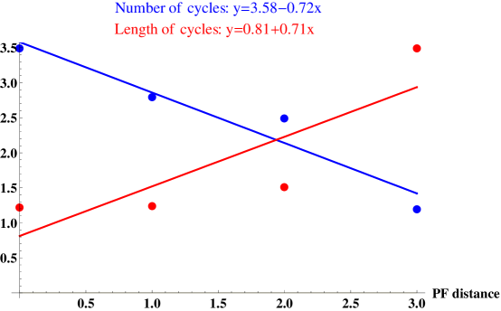
Figure 3:

Table 2:

n	Num. of Exp.	Av. Num.	Av. Len.
5	117000	99.75	99.83
7	5000	97.82	99.92
10	6000	95.70	99.58
15	2921	95.72	98.25
20	331	90.03	94.86
100	659	77.39	93.93

Table 3:

$D$	Av. Num.	Av. Len.	Med. Num.	Med. Len.
$25\%$	26	114	29	542
$50\%$	4	16	18	59
$75\%$	0	1	6	3
$100\%$	1	0	2	0

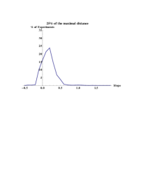
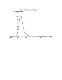
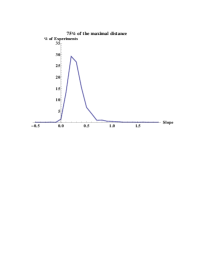
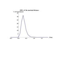
Figure 4:

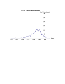
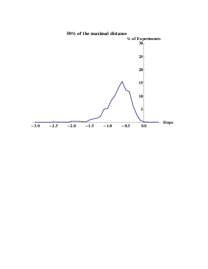
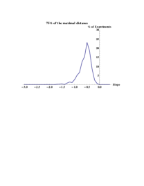
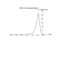
Figure 5:

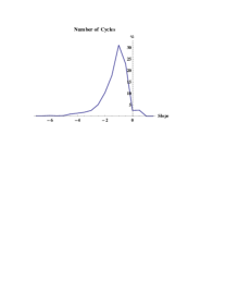
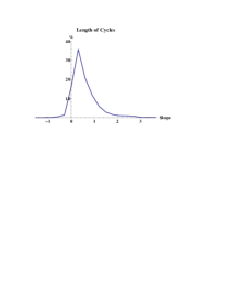
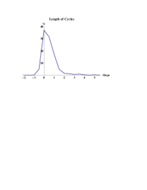
Figure 6:

References

- Thomas et al. (1995) Thomas, R., D. Thieffry, and M. Kaufman, 1995. Dynamical behaviour of biological regulatory networksI. Biological role of feedback loops and practical use of the concept of the loop-characteristic state. Bulletin of Mathematical Biology 57:247–276.
- Soule (2003) Soule, C., 2003. Graphic requirements for multistationarity. ComPlexUs 1:123–133.
- Plahte et al. (1995) Plahte, E., T. Mestl, and S. Omholt, 1995. Feedback loops, stability and multistationarity in dynamical systems. Journal of Biological Systems 3:409–413.
- Gauzé (1998) Gauzé, J., 1998. Positive and negative circuits in dynamical systems. Journal of Biological Systems 6:11–15.
- Cinquin and Demongeot (2002) Cinquin, O., and J. Demongeot, 2002. Positive and Negative Feedback: Striking a Balance Between Necessary Antagonists. Journal of Theoretical Biology 216:229–241.
- Angeli et al. (2007) Angeli, D., M. Hirsch, and E. Sontag, 2007. Attractors in monotone cascades of differential equations. Submitted.
- Sontag (2005) Sontag, E., 2005. Molecular systems biology and control. Eur. J. Control 11:396–435.
- Kauffman (1969a) Kauffman, S., 1969. Metabolic stability and epigenesis in randomly constructed genetic nets. J. Theor. Biol. 22:437–467.
- Kauffman (1969b) Kauffman, S., 1969. Homeostasis and differentiation in random genetic control networks. Nature 224:177–178.
- Kauffman and Glass (1973) Kauffman, S., and K. Glass, 1973. The logical analysis of continuous, nonlinear biochemical control networks. Journal of Theoretical Biology 39:103–129.
- Albert and Othmer (2003) Albert, R., and H. Othmer, 2003. The topology of the regulatory interactions predicts the expression pattern of the Drosophila segment polarity genes. J. Theor. Biol. 223:1–18.
- Chaves et al. (2005) Chaves, M., R. Albert, and E. Sontag, 2005. Robustness and fragility of Boolean models for genetic regulatory networks. J. Theoret. Biol. 235:431–449.
- Gilbert (1954) Gilbert, E., 1954. Lattice theoretic properties of frontal switching functions. Journal of Mathematics and Physics 33:57–67.
- Minsky (1967) Minsky, M., 1967. Computation: finite and infinite machines. Prentice-Hall, Englewood Cliffs, N.J.
- Aracena et al. (2004a) Aracena, J., J. Demongeot, and E. Goles, 2004. On limit cycles of monotone functions with symmetric connection graph. Theor. Comput. Sci. 322:237–244.
- Aracena et al. (2004b) Aracena, J., J. Demongeot, and E. Goles, 2004. Positive and negative circuits in discrete neural networks. IEEE Trans Neural Networks 15:77–83.
- Goles and Hernández (2000) Goles, E., and G. Hernández, 2000. Dynamical behavior of Kauffman networks with AND-OR gates. Journal of Biological Systems 8:151–175.
- Smith (1995) Smith, H., 1995. Monotone dynamical systems: An introduction to the theory of competitive and cooperative systems, Mathematical Surveys and Monographs, vol. 41. AMS, Providence, RI.
- Anderson (2002) Anderson, I., 2002. Combinatorics of Finite Sets. Dover Publications, Mineola, N.Y.
- Tosic and Agha (2004) Tosic, P. T., and G. Agha, 2004. Characterizing Configuration Spaces of Simple Threshold Cellular Automata. In ACRI. 861–870.
- Greil and Drossel (2007) Greil, F., and B. Drossel, 2007. Kauffman networks with threshold functions. European Physical Journal B 57:109–113.
- Kwon and Cho (2007) Kwon, Y.-K., and K.-H. Cho, 2007. Boolean Dynamics of Biological Networks with Multiple Coupled Feedback Loops. Biophysical Journal 92:2975–2981.
- DasGupta et al. (2007) DasGupta, B., G. Enciso, E. Sontag, and Y. Zhang, 2007. Algorithmic and complexity aspects of decompositions of biological networks into monotone subsystems. BioSystems 90:161–178.
- Sontag (2007) Sontag, E., 2007. Monotone and near-monotone biochemical networks. Journal of Systems and Synthetic Biology 1:59–87.
- Maayan et al. (2007) Maayan, A., R. Iyengar, and E. D. Sontag, 2007. Intracellular Regulatory Networks are close to Monotone Systems. Technical Report npre.2007.25.1, Nature Precedings.
- Hadeler and Glas (1983) Hadeler, K., and D. Glas, 1983. Quasimonotone systems and convergence to equilibrium in a population genetics model. J. Math. Anal. Appl. 95:297–303.
- Hirsch (1984) Hirsch, M., 1984. The dynamical systems approach to differential equations. Bull. A.M.S. 11:1–64.
- Hirsch and Smith (2005) Hirsch, M., and H. Smith, 2005. Monotone dynamical systems. In Handbook of Differential Equations, Ordinary Differential Equations (second volume), Elsevier, Amsterdam.
- Dancer (1998) Dancer, E., 1998. Some remarks on a boundedness assumption for monotone dynamical systems. Proc. of the AMS 126:801–807.
- Hirsch (1983) Hirsch, M., 1983. Differential equations and convergence almost everywhere in strongly monotone flows. Contemporary Mathematics 17:267–285.
- Hirsch (1985) Hirsch, M., 1985. Systems of differential equations that are competitive or cooperative II: Convergence almost everywhere. SIAM J. Mathematical Analysis 16:423–439.
- Dasgupta et al. (2006) Dasgupta, B., G. Enciso, E. Sontag, and Y. Zhang, 2006. Algorithmic and complexity results for decompositions of biological networks into monotone subsystems. In Lecture Notes in Computer Science: Experimental Algorithms: 5th International Workshop, WEA 2006, Springer-Verlag, 253–264. (Cala Galdana, Menorca, Spain, May 24-27, 2006).
- Hüffner et al. (2007) Hüffner, F., N. Betzler, and R. Niedermeier, 2007. Optimal edge deletions for signed graph balancing. In Proceedings of the 6th Workshop on Experimental Algorithms (WEA07), June 6-8, 2007, Rome, Springer-Verlag.
- Zaslavsky (1998) Zaslavsky, T., 1998. Bibliography of signed and gain graphs. Electronic Journal of Combinatorics DS8.
- Harary (1953) Harary, F., 1953. On the notion of balance of a signed graph. Michigan Mathematical Journal 2:143–146.
- Jarrah et al. (2004) Jarrah, A., R. Laubenbacher, and H. Vastani, 2004. DVD: Discrete Visual Dynamics. World Wide Web. http:dvd.vbi.vt.edu.