The traveling wave approach to asexual evolution: Muller’s ratchet and speed of adaptation

Abstract

We use traveling-wave theory to derive expressions for the rate of accumulation of deleterious mutations under Muller’s ratchet and the speed of adaptation under positive selection in asexual populations. Traveling-wave theory is a semi-deterministic description of an evolving population, where the bulk of the population is modeled using deterministic equations, but the class of the highest-fitness genotypes, whose evolution over time determines loss or gain of fitness in the population, is given proper stochastic treatment. We derive improved methods to model the highest-fitness class (the stochastic edge) for both Muller’s ratchet and adaptive evolution, and calculate analytic correction terms that compensate for inaccuracies which arise when treating discrete fitness classes as a continuum. We show that traveling wave theory makes excellent predictions for the rate of mutation accumulation in the case of Muller’s ratchet, and makes good predictions for the speed of adaptation in a very broad parameter range. We predict the adaptation rate to grow logarithmically in the population size until the population size is extremely large.

1 Introduction

“I was observing the motion of a boat which was rapidly drawn along a narrow channel by a pair of horses, when the boat suddenly stopped—not so the mass of water in the channel which it had put in motion; it accumulated round the prow of the vessel in a state of violent agitation, then suddenly leaving it behind, rolled forward with great velocity, assuming the form of a large solitary elevation, a rounded, smooth and well-defined heap of water, which continued its course along the channel apparently without change of form or diminution of speed.” (Russell, 1845)

One of the fundamental models of population genetics is that of a finite, asexually reproducing population of genomes consisting of a large number of sites with multiplicative contribution to the total fitness of the genome. This model has been studied for decades, and has presented substantial challenges to researchers trying to solve it analytically. Even in its most basic formulation, where each site is under exactly the same selective pressure, the model has not been fully solved to this day. For the special case of vanishing back mutations, the model reduces to the problem of Muller’s ratchet (Muller, 1964; Felsenstein, 1974). A tremendous amount of research effort has been directed at this problem (Haigh, 1978; Pamilo et al., 1987; Stephan et al., 1993; Higgs and Woodcock, 1995; Gordo and Charlesworth, 2000a, b; Rouzine et al., 2003). Other special cases of this model are mutation–selection balance when the forward and back mutation rates are equal (Woodcock and Higgs, 1996), and the speed of adaptation under various conditions (Tsimring et al., 1996; Kessler et al., 1997; Gerrish and Lenski, 1998; Orr, 2000; Rouzine et al., 2003; Wilke, 2004).

In 1996, Tsimring et al. pioneered a new approach to studying the multiplicative multi-site model. They described the evolving population as a localized traveling wave in fitness space, using partial differential equations developed to describe wave-like phenomena in physical systems. A traveling wave is a localized profile traveling at near-constant speed and shape (physicists refer to such phenomena also as solitary waves). We can envision a population as a traveling wave of the distribution of the mutation number over genomes if the relative mutant frequencies in the population stay approximately constant while the population shifts as a whole. For example, a population may have specific abundances of sequences at one, two, three, or more mutations away from the least loaded class at all times, but the least-loaded class moves at constant speed by one mutation every ten generations.

Encouraging results by Tsimring et al. (1996) were based on two strong approximations. Firstly, all fitness classes, including the best-fit class, were described deterministically, neglecting random effects due to finite population size. Finite population size was introduced into the problem as a cutoff of the effect of selection at the high-fitness edge, when the size of a class becomes less than one copy of a genome. Secondly, Tsimring et al. (1996) approximated the traveling wave profile with a function continuous in fitness (or mutation load). In these approximations, Tsimring et al. (1996) demonstrated the existence of a continuous set of waves with different speeds. The cutoff condition determined the choice of a specific solution and the dependence of the speed on the population size.

Rouzine et al. (2003) confirmed the qualitative conclusions by Tsimring et al. (1996) and refined their quantitative results in two ways, by taking into account the random effects acting on the smallest, best-fit class, and showing that, in a broad parameter range, approximating the logarithm of the wave profile as a smooth function of the fitness is a much better approximation than approximating the wave profile itself as a smooth function. It was shown that the substitution rate increases logarithmically with the population size, until the deterministic single-site limit is reached at extremely large population sizes and the theory breaks down.

The purpose of the present paper is to show that the results by Rouzine et al. (2003) can still be improved regarding both the treatment of the high-fitness edge and the deterministic part of the fitness distribution. Because the original work was presented in an extremely condensed format, we will here re-derive the general theory in detail. Then, we will present improved treatments of the stochastic edge that lead to accurate predictions for the substitution rate defined as the average gain in beneficial alleles per genome per generation. We consider in detail two opposite parametric limits, Muller’s ratchet (when beneficial mutation events are not important) and adaptive evolution (when deleterious mutations are not important).

Because the range of validity of our approach caused some confusion in the literature, we discuss it in detail in the main text and Appendix. Briefly, both in Muller’s ratchet and in the adaptation regime, we assume that the total number of sites is large, and the selection coefficient $s$ is small. The population size $N$ should be sufficiently large, so that the difference in the mutational load between the least-loaded and average genomes is much larger than 1. In other words, a large number of sites are polymorphic at any time. For the adaptive evolution, the condition corresponds to the average substitution rate $V$ being much larger than $s/\ln(V/U_{\text{b}})$, where $U_{\text{b}}$ is the beneficial mutation rate, or population sizes being much larger than $\sqrt{s/U_{b}^{3}}/\ln(V/U_{b})$. We also assume that $V$ is much larger than $U_{b}$. In smaller populations, adaptation occurs by isolated selective sweeps at different sites, and one-site models apply. Two-site models of adaptation, such as the clonal interference theory (Gerrish and Lenski, 1998; Orr, 2000; Wilke, 2004), can be used to describe the narrow transitional interval in $N$. Further, if the deleterious mutation rate per genome is much larger than $s$, and the average population fitness is sufficiently high, an additional broad interval of $N$ appears, where deleterious mutations accumulate (Muller’s ratchet). Using numeric simulations and analytic estimates, we demonstrate good accuracy of our results in a very broad parameter range relevant for various asexual organisms, including asexual RNA and DNA viruses, yeast, some plants, and fish.

The manuscript is organized as follows. In Section 2, we describe the model and the general method to derive evolutionary dynamics in terms of the fitness distribution. In Section 3 and 4, we consider in detail two particular cases, Muller’s ratchet and the process of adaptation, respectively, and test analytic results with computer simulations. In Section 4, we discuss our findings.

2 Traveling-wave theory

2.1 Model assumptions

We consider a multi-site model of $L$ sites, where each site can be in two states, i.e., carry one of two alleles, either advantageous or deleterious. The deleterious allele reduces the overall fitness of a genome by a factor of $1-s$, where $s\ll 1$ is the selective disadvantage per site. We assume that there are no biological interactions between sites (epistasis), so that the fitness of a genome with $k$ deleterious alleles (mutational load) is $(1-s)^{k}\approx e^{-ks}$. We refer to the frequency of sequences with mutational load $k$ in the population as $f_{k}$, and write the population-average fitness as $w_{\text{av}}=\sum_{k}e^{-sk}f_{k}$. We introduce $k_{\text{av}}$, which is mutational load for which a sequence’s fitness is exactly equal to the population mean fitness, as given by $w_{\text{av}}=e^{-sk_{\text{av}}}$. For small $s$, $k_{\text{av}}$ is approximately the average mutational load in the population, $k_{\text{av}}\approx\sum_{k}kf_{k}$. We denote the mutational load of the best-fit sequence in the population as $k_{0}$. Note that in general $k_{0}\neq 0$, that is, the best- fit sequence in the population is not the sequence with the overall highest possible fitness.

We assume that an allele can mutate into an opposite allele with a small probability $\mu$. For the sake of simplicity of the derivation, we assume that the mutation rate is low, so that there is, at most, one mutation per genome per generation. The case when multiple mutations per genome are frequent takes place at very large population sizes when the average substitution rate is high, larger than one new beneficial allele per generation. Rouzine et al. (2003) considered this more general case and showed that there is no essential change in the final expression for the substitution rate. Thus, for finite population size, the assumption of a single mutation per genome per round of replication is not limiting (see also the next subsection).

In real genomes, $s$ varies between sites. Moreover, Gillespie (1983, 1991) and Orr (2003) argued that the distribution of $s$ differs between sites with beneficial and deleterious alleles. A viable genome represents a highly-fit, non-random selection of alleles, so that deleterious mutations should generally have larger effects than beneficial mutations. For the same reason, these authors predicted that the effective distribution of $s$ for beneficial alleles should have a universal exponential form. In the present work, we do not consider variation in $s$. Instead, we use a simplified model including only those sites into the total number of sites $L$ —with either deleterious and beneficial alleles— whose selection coefficient is on the order of the same typical value $s$, and approximate all selection coefficients at these sites with a constant $s$. The choice of $s$ and, hence, of the set of included sites depends on the time scale of evolution under consideration. Strongly deleterious mutations with effects much larger than $s$ are cleared rapidly from a population. Strongly beneficial mutations are fixed at the early stages of evolution. Note that in the “clonal interference” approximation (Gerrish and Lenski, 1998), which considers competition between two beneficial clones emerging at two sites, variation of $s$ must be taken into account to make continuous adaptation possible. In contrast, in the present theory, which allows new beneficial clones to grow inside of already existing clones, the importance of variation in $s$ is less obvious. We hope to address this matter elsewhere.

We discuss the validity of our approach in detail for the limits of Muller’s ratchet and adaptation and give a summary of the central simplifications—numbered 1 through 6 and referenced throughout the text—in the Appendix. Note that we can verify the validity of the various assumptions only after the fact, once we have obtained our final results. All simplifications are asymptotically exact, i.e., are based on the existence of small dimensionless parameters. The most limiting requirements are that the high-fitness tail of the distribution is long, and that the distribution is far from the unloaded and fully loaded (possible best-fit and less-fit) genomes.

2.2 General approach

The first idea underlying the approach of ”solitary wave” is to classify all genomes in a population according to their fitness (mutational load), regardless of specific locations of deleterious alleles in a genome, and focus on evolution of fitness classes. The second idea is to describe evolution of most fitness classes deterministically. To take into account the effects of finite population size, such as genetic drift and randomness of mutation events, only one class with the highest fitness is described stochastically using the standard two-allele diffusion approach. The best-fit class is considered a minority ”allele” in a population, and all other sequences are considered the majority ”allele”. The reason why stochastic effects can be neglected already for the next-to-best class is that, in a broad parameter range, the fitness distribution decreases exponentially towards the stochastic edge. Hence, the next-to-best class is large enough to neglect stochastic effects, especially in the adaptation regime (see estimates in Sections 3 and 4).

We note that neglecting stochastic effects completely and considering the limit of infinite population is not correct. As we show below, stochastic processes acting on the best-fit class limit the overall evolution rate and make it dependent on the population size. Even for a modest number of sites ($L$ = 15-20), the substitution rate is predicted to reach the true deterministic limit only in astronomically large populations not found in nature (Tsimring et al., 1996; Rouzine et al., 2003; Desai and Fisher, 2007). For the same reason, the assumption of one mutation per genome we made in our model is not a limiting factor and, as shown by Rouzine et al. (2003), does not change much in the final expression for the average substitution rate.

The formal procedure consists of several steps, as follows.

(i) The frequencies of all fitness classes excluding the best-fit class are described by a deterministic balance equation.

(ii) The equation is shown to have a traveling wave solution with an arbitrary speed (the average substitution rate).

(iii) The leading front of the wave (high-fitness tail of the distribution) is shown to end abruptly at a point, expressed in terms of the wave speed.

(iv) The difference between the values of the fitness distribution at the center and the edge is expressed in terms of the wave speed.

(v) The value at the center is found from the normalization condition.

(vi) Because the biological justification for the lack of genomes beyond the high-fitness cutoff is finite size of population, the cutoff point is identified with the stochastic edge.

(vii) To determine the wave speed as a function of the population size, the average frequency of the least-loaded class is estimated from the classical diffusion result and matched to the deterministic cutoff value.

2.3 Equation for the deterministic part of the fitness distribution

We proceed with the first step. On the basis of our model assumptions and neglecting multiple mutation events per generation per genome, we can write the deterministic time evolution of the frequency $f_{k}(t)$ of genomes with mutational load $k$ as

$$f_{k}(t+1) =\frac{1}{w_{\text{av}}(t)}\Big{(}e^{-s(k-1)}\mu(L-k+1)f_{k-1}(t)$$

$$\quad+e^{-s(k+1)}\mu(k+1)f_{k+1}(t)+e^{-sk}(1-\mu L)f_{k}(t)\Big{)}\,,$$ (1)

where $k$ runs from 0 to $L$ and $f_{-1}(t)\equiv f_{L+1}(t)\equiv 0$. By definition, $\sum_{k}f_{k}(t)=1$ for all times $t$. Now we introduce the total per-genome mutation rate $U=\mu{}L$, and the ratio of beneficial mutation rate per genome to the total mutation rate, $\alpha_{k}=\mu{}k/U=k/L$. Inserting these expressions into Eq. (2.3), expressing $w_{\text{av}}$ in terms of $k_{\text{av}}$, expanding $e^{-sx}\approx 1-sx$ (which we are allowed to do under the condition that $s|k-k_{\text{av}}|\ll 1$, Simplification 1), and neglecting all terms proportional to $sU$, we arrive at:

$$f_{k}(t+1) =U(1-\alpha_{k-1})f_{k-1}(t)+U\alpha_{k+1}f_{k+1}(t)$$

$$\qquad\qquad\qquad\qquad+[1-U-s(k-k_{\text{av}})]f_{k}(t)\,.$$ (2)

As mentioned before, we consider the case when the traveling wave is far from the sequence with the highest possible fitness, $k=0$, as given by the condition $|k-k_{\rm av}|\ll k_{\rm av}$. Therefore, $\alpha_{k}$ depends only slowly (linearly) on $k$, we are allowed to replace $\alpha_{k}$ by $\alpha\equiv\alpha_{k_{\text{av}}}$ (Simplification 2), and find

$$f_{k}(t+1)-f_{k}(t)=U(1-\alpha)f_{k-1}(t)+U\alpha f_{k+1}(t)-[U+s(k-k_{\text{av}})]f_{k}(t)\,.$$ (3)

Our goal is to turn this expression into a continuous differential equation. As the mutation rates are low, $f_{k}(t)$ evolves very slowly in time, and we can write $f_{k}(t+1)\approx f_{k}(t)+\partial f_{k}(t)/\partial t$ (Simplification 3).

We need to be more careful when making a continuous approximation for $f_{k}(t)$ as a function of $k$. As we show below, $f_{k}(t)$ changes rapidly with $k$ in the important high fitness tail. Therefore, the Taylor expansion of $f_{k}(t)$ is not justified. However, the logarithm of $f_{k}(t)$ is a smooth function of $k$ in a broad parameter range, provided the ”lead” of the distribution is large (Simplification 4). [The lead is the difference in number of mutations from the population center to the least-loaded class in the population (Desai and Fisher, 2007).] Therefore, a better approximation, which represents an improvement on the work by Tsimring et al. (1996), is to do the Taylor expansion on $\ln f_{k}$ and write $f_{k+1}(t)=f_{k}(t)\exp[\partial\ln f_{k}(t)/\partial k]$. With these approximations, and after introducing a rescaled time $d\tau=Udt$ and a rescaled selection coefficient $\sigma=s/U$, we find

$$\partial\ln f_{k}(t)/\partial\tau=(1-\alpha)e^{-\partial\ln f_{k}(t)/\partial k}+\alpha e^{\partial\ln f_{k}(t)/\partial k}-\sigma(k-k_{\text{av}})-1\,.$$ (4)

This nonlinear partial differential equation describes the deterministic movement of the population in fitness space over time.

(Note that, for sufficiently large $N$, the assumptions of Simplifications 1 and 3 may be violated, so that technically, we can neither expand fitness in $k$ nor replace discrete time with continuous time in this regime. Nevertheless, Rouzine et al. (2003) showed that the continuous equation for the fitness distribution, Eq. (4), can be derived in a more general way, without assuming $\partial\ln f_{k}(t)/\partial t\ll 1$, nor expanding fitness in $k$, nor neglecting multiple mutations per genome per generation [see the transition from Eq. (1) to Eq. (11) in the Supplementary Text of the quoted work]. In the present work, we use these approximations only to simplify our derivation.)

In the equation above, $\alpha$ and $\sigma$ depend, strictly speaking, on time. The dependence is, however, very weak in the limit of a large genome size $L$. In the remainder of this paper, we shall assume that the observation time is very small compared to the time in which $k_{\text{av}}$ changes by $L$ and, thus, $\alpha$ and $\sigma$ can be considered constant. At the same time, because the distribution is very far from the class without deleterious alleles, $|k-k_{\text{av}}|\ll k_{\text{av}}$, a considerable shift of the distribution can occur during the observation time.

2.4 Traveling wave solution

A broad class of partial differential equations affords solutions in the form of traveling waves. A wave is a fixed shape, described by a function $\phi(x)$, that moves through space without changing its form. In the case of an evolving population, space corresponds to the mutational load, $k$. A traveling wave solution to Eq. (4) can be expressed as the movement of the center of the population over time, $k_{\text{av}}(\tau)$, and the shape of the wave around this center, which we write as $\phi[k-k_{\text{av}}(\tau)]$. We therefore make the ansatz (Simplification 5) that

$$\ln f_{k}(t)=\phi[k-k_{\text{av}}(\tau)]\,$$ (5)

After inserting Eq. (5) into Eq. (4) and writing $x=k-k_{\text{av}}(\tau)$, we obtain

$$\sigma x=(1-\alpha)e^{-\phi^{\prime}(x)}+\alpha e^{\phi^{\prime}(x)}+v\phi^{\prime}(x)-1\,,$$ (6)

where $\phi^{\prime}(x)=\partial\phi(x)/\partial x$, and we have introduced the wave velocity $v$, that is, the speed of movement of the population center $k_{\text{av}}$ over time, $v\equiv\partial k_{\text{av}}(\tau)/\partial\tau$.

For a given wave velocity $v$, Eq. (6) and $\phi(0)$ fully specify the shape of the wave $\phi(x)$. Although it is not possible to solve Eq. (6) in the general form, analytically, below we will be able to find the velocity of the wave. The first step is to derive $\phi(0)$ from the normalization condition.

2.5 Normalization condition. Width and speed

The validity of the approach by Rouzine et al. (2003) requires that the logarithm of the fitness distribution, $\phi(x)$, can be approximated with a smooth function of $x$. In other words, the characteristic scale in $x$ given by the length of the high-fitness tail is much larger than unit. The condition is always met when population is evolving at many sites at a time. Because the fitness distribution itself, $\exp[\phi(x)]$, is not replaced with a smooth function of $x$, it does not have to be broad: Whether the half-width of the wave is small or large is irrelevant for the validity of the approach. In the treatment of adaptation limit (Section 4), the wave can be either broad or narrow, depending on the range of population sizes. The two cases, however, have different normalization conditions, as follows.

If the wave is narrow, $\text{Var}[k]=\text{Var}[x]\ll 1$, most of the distribution is localized at $k\approx k_{\text{av}}$, and from the normalization sum $\sum_{k=0}^{L}{f_{k}(t)}$ we have

$$\phi(0)\approx 0.$$ (7)

(The exception is the case when $k_{\text{av}}$ is nearly half-integer, and the two adjacent classes have comparable sizes.)

If the wave is broad, $\text{Var}[k]\gg 1$, the normalization condition is less trivial. The normalization sum $\sum_{k=0}^{L}{f_{k}(t)}$ can be replaced with an integral, $\int{e^{\phi(x)}dx}$. As we will see momentarily, the main contribution to the integral comes from the interval of $x$ such that $|x|$ is much larger than 1 but much smaller than the high-fitness tail length, so that $|\phi^{\prime}(x)|\ll 1$. Hence, we can expand the exponential terms in Eq. (6) to the first order (Simplification 6), and find

$$\phi^{\prime}(x)=-\frac{\sigma x}{1-2\alpha-v}\,.$$ (8)

Clearly, $|\phi^{\prime}(x)|\ll 1$ when $|x|\ll(1-2\alpha-v)/\sigma$, and therefore this latter condition determines the validity of Eq. (8). Integrating in $x$, taking into account the normalization condition, we obtain the expression for $\phi(x)$ near the wave center

$$\phi(x)=\ln\sqrt{\frac{\sigma}{2\pi(1-2\alpha-v)}}-\frac{\sigma x^{2}}{2(1-2\alpha-v)}\,.$$ (9)

In particular, the desired expression for $\phi(0)$ has a form

$$\phi(0)=\ln\sqrt{\frac{\sigma}{2\pi(1-2\alpha-v)}}.$$ (10)

Note that $\phi(x)$ was defined as $\phi(x)=\ln f_{k}(t)$. Therefore, Eq. (9) implies that the distribution of genomes in the vicinity of $k_{\text{av}}$ is approximately Gaussian, with variance

$$\text{Var}[k]=(1-2\alpha-v)/\sigma\,.$$ (11)

Because the variance and the argument of the square root in Eq. (10) must be positive, the wave velocity has to satisfy $v<1-2\alpha$. In other words, if deleterious mutations accumulate, the rate of their accumulation cannot exceed $1-2\alpha$ if time is measured in units of $U$. Also, as we already stated, the Gaussian expression for the central part of the wave is valid if the width of the wave $\sqrt{\text{Var}[k]}$ is much larger than 1. For moderate or small wave speeds, $|v|\sim 1$ or $|v|\ll 1$, this condition implies that $\sigma$ is much smaller than 1. Whether the wave is actually narrow or broad, given the population size and other parameters, will be discussed below for Muller’s ratchet and the adaptation regime.

Eq. (11), which is known as Fisher Fundamental Theorem, links the width of the population’s mutant distribution, $\sqrt{\text{Var}[k]}$, to the velocity $v$ at which the wave is traveling. We emphasize that the validity of this expression is not restricted to the case of broad fitness distribution and can be derived directly from Eq. (3) (Appendix) even if $\text{Var}[k]\ll 1$. Qualitatively, the theorem states that, the broader the wave, the larger the characteristic difference in fitness between two representative genomes, and the stronger the effect of positive selection on the substitution rate.

2.6 High-fitness edge of distribution

In the previous subsections, we have derived a continuous wave equation that gives a deterministic description of how the bulk of the population moves over time in fitness space. However, the speed of the wave remains undefined. As it turns out, the behavior of a small class of best-fit genomes determines the speed.

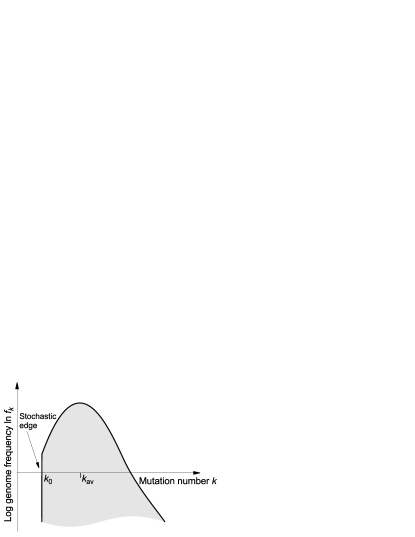
Figure 1: Schematic illustration of the solitary wave profile. The stochastic edge is the minimum-$k$ boundary of the population’s mutant distribution. There are no genomes with fewer than $k_{0}$ mutations in the population. The speed of the wave is primarily determined by how fast mutations are gained or lost at the stochastic edge.

Below we show that the deterministic wave has a cutoff in the high-fitness tail of the wave whose position is defined by the wave speed and model parameters. The biological reason behind the deterministic cutoff are stochastic factors acting on finite populations. Highly-fit genomes are either gradually lost (Muller’s ratchet) or gradually gained (adaptation) by a population. Thus, the deterministic cutoff is identified with the ”stochastic edge” of the wave that gradually advances or retreats (Fig. 1). The rate of the loss or gain of the least-loaded class, which depends on the population size, ultimately determines the speed of the wave. To obtain the desired condition for the wave speed, in the next subsection, we will match the deterministic description to stochastic behavior of the least-loaded class.

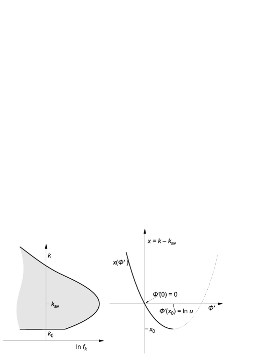
Figure 2: The minimum of the function $x(\phi^{\prime})$ determines the location of the stochastic edge, $k_{0}$.

We cannot solve Eq. (6) explicitly. Fortunately, we can extract the location of the stochastic edge by interpreting Eq. (6) as an equation that describes a function $x(\phi^{\prime})$ rather than a function $\phi^{\prime}(x)$. If the function $x(\phi^{\prime})$ has an absolute minimum, then this minimum implies that $\phi(x)$ has a deterministic cutoff, and thus the minimum must coincide with the stochastic edge (Fig. 2).

Therefore, consider the function $x(\phi^{\prime})=[(1-\alpha)e^{-\phi^{\prime}}+\alpha e^{\phi^{\prime}}+v\phi^{\prime}-1]/\sigma$. Clearly, $x(\phi^{\prime})\rightarrow\infty$ for $\phi^{\prime}\rightarrow\pm\infty$, as long as $0<\alpha<1$ or $\alpha=0$ and $v>0$. To locate any minima, we calculate the derivative $dx(\phi^{\prime})/d\phi^{\prime}$, and find

$$\frac{dx(\phi^{\prime})}{d\phi^{\prime}}=[-(1-\alpha)e^{-\phi^{\prime}}+\alpha e^{\phi^{\prime}}+v]/\sigma=0\,.$$ (12)

We solve the resulting quadratic equation in $e^{\phi^{\prime}}$ and arrive at

$$e^{\phi^{\prime}}=\frac{1}{2\alpha}\Big{[}-v+\sqrt{v^{2}+4\alpha(1-\alpha)}\Big{]}\equiv u\,.$$ (13)

The alternative solution, with a minus sign in front of the square root, is not possible for real-valued $\phi^{\prime}$. Thus, the derivative of $x(\phi^{\prime})$ has only a single root, which must correspond to an absolute minimum. The value of $x(\phi^{\prime})$ at this minimum, which we denote by $x_{0}$, follows as

$$x_{0}=-\frac{1}{\sigma}(1-2\alpha u-v\ln u-v)\,,$$ (14)

where we have made use of the identity $(1-\alpha)/u=\alpha u+v$. For any mutation classes $k$ corresponding to $x<x_{0}$, we have $f_{k}\equiv 0$. For the continuous approach to work, we need $|x_{0}|\gg 1$ (Simplification 4).

2.7 Difference between fitness distribution at center and edge

Our eventual goal is to find an expression that relates the speed of the wave, $v$, to the population size $N$, mutation rate $U$, selective coefficient $s$, and the fraction of beneficial mutations $\alpha$. It turns out that we can achieve this goal by considering the difference $\phi(0)-\phi(x_{0})$. By evaluating this difference in two alternative ways, we end up with the desired relation.

First, we note that

$$\phi(0)-\phi(x_{0})=\int_{x_{0}}^{0}\phi^{\prime}(x)dx\,.$$ (15)

We can evaluate the integral on the right-hand side by making the subsitution $x=x(\phi^{\prime})$, integrating by parts, and using $\phi^{\prime}(x_{0})=\ln u$ and $\phi^{\prime}(0)=0$. (The former condition stems from the definition of $u$, while the latter condition is a consequence of Eq. (8); see also Fig. 2.) We arrive at

$$\phi(0)-\phi(x_{0})=-x_{0}\ln u-\int_{\ln u}^{0}x(\phi^{\prime})d\phi^{\prime}\,.$$ (16)

We can evaluate the remaining integral on the right-hand side by integrating over Eq. (6) . We obtain, after inserting Eq. (14) into the first term on the right-hand side of Eq. (16),

$$\phi(0)-\phi(x_{0})=\frac{1}{\sigma}\Big{(}1-2\alpha-\frac{v}{2}[\ln^{2}(eu)+1]-2\alpha u\ln u\Big{)}\,,$$ (17)

where $e$ is Euler’s constant, $\ln(e)=1$.

We have now calculated $\phi(0)-\phi(x_{0})$ by integrating over $\phi^{\prime}(x)$. Alternatively, we can calculate this difference by evaluating $\phi(x)$ directly at 0 and at $x_{0}$. $\phi(0)$ follows from Eq. (10) if the argument of the logarithm is much smaller than 1 (large half-width of the wave), and $\phi(0)=0$ in the opposite limit (small half-width). The quantity $\phi(x_{0})$ represents the logarithm of the genome frequency right at the stochastic edge. Since this value is dominated by stochastic effects, we cannot evaluate $\phi(x_{0})$ on the basis of the deterministic theory we have developed so far. Therefore, we proceed as follows. We give the genome frequency at the stochastic edge proper stochastic treatment and base our estimate of the expected genome frequency at the stochastic edge on these probabilistic arguments.

2.8 Stochastic treatment of the least-loaded class

The deterministic derivation in the previous subsections demonstrates the existence of a continuous set of solitary waves with various speeds, i.e., average substitution rates. Now, to choose the correct solution and determine the actual substitution rate, we have to take into account stochastic effects acting on the least-loaded class, $k=k_{0}$. At this point, finite population size enters the scene. We describe the dynamics of the least-loaded class using the one-site, two-allele model (see reviews in Kimura (1964), Rouzine et al. (2001), or Ewens (2004)). The frequency of the least-loaded class is analogous to the concentration of the better-fit allele. To justify the deterministic treatment of the next-loaded class (and other classes) and estimate the error introduced by that approximation, we will estimate its size in the limits of adaptation and Muller’s ratchet in Sections 3 and 4, respectively.

The accurate treatment of the stochastic dynamics of least-loaded class, $f_{k_{0}}(t)$, requires the use of a diffusion equation that includes both deterministic factors (selection and mutation) and random genetic drift. For the purpose of the present work, a good accuracy can be ensured by a simpler approach, as follows.

A well-known fact following from the diffusion equation is that deterministic factors dominate when the frequency of a minority allele in a population (in our case, $f_{k_{0}}(t)$) is much larger than $1/(N|S|)$ (Maynard Smith, 1971; Barton, 1995; Rouzine et al., 2001); in the opposite case, random drift rules, and the minority is most likely to be lost. Here $\exp(|S|)$ is the fitness advantage of the better-fit allele. If the best-fit class is much larger than that value, we can use the deterministic equation, Eq. (3), which yields

$$\partial f_{k_{0}}/\partial t=M(t)-Sf_{k_{0}}(t)$$ (18)

with $M(t)=U\alpha f_{k_{0}+1}(t)$ and $S=U+s(k_{0}-k_{\text{av}})$. The parameter $S$ represents the effective coefficient of selection against the best-fit class in the population. It consists of two parts: the positive part $U$ due to mutations removing genomes from the class, and the negative part due to the fitness difference between the least-loaded sequence and the average genome, $s(k_{0}-k_{\text{av}})$.

As we show below, $S$ is positive and $M$ is negligible in the ratchet limit, $v>0$, and negative in the adaptation limit, $v<0$, where $M(t)$ is more pronounced but still relatively small. In the ratchet limit, the least-loaded class decreases exponentially until it hits the characteristic size $1/(N|S|)$ and is lost. In the adaptation limit, the least loaded class is created due to a mutation and becomes established, i.e., survives and grows further with probability on the order of $1/2$, when its frequency in a population exceeds $1/(N|S|)$. The cost of treating a characteristic frequency $1/(N|S|)$ as a sharp threshold is an undefined numeric factor multiplying the population size, $N$. Because the speed of evolution, as it comes out in the end, depends on $N$ logarithmically, and the interesting values of $N$ are quite large, the error is relatively small.

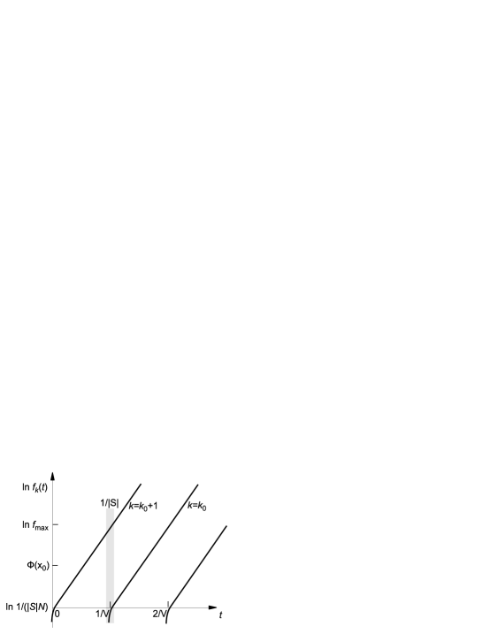
Figure 6: Schematic illustration of establishment of a new best-fit class. Once a beneficial mutant has survived drift, its frequency grows approximately exponentially in time. A further beneficial mutation is likely to arise and survive drift only in a short time interval of length $1/S$ around the time when the currently least-loaded class has grown to its maximal value $f_{\max}$.

The deterministic formalism described in the previous section predicts a monotonous dependence on time for a fitness class (the time derivative changes sign only at $k=k_{\rm av}$). In fact, because the mutational load of the least-loaded class $k_{0}$ changes abruptly in time, the size of the current least-loaded class oscillates in time producing a saw-like dependence. In the case of the Muller’s-ratchet, the class contracts until lost (Fig. 3), and the next-loaded class takes it place, and in the case of adaptation, the class expands until beneficial mutations create a new least-loaded class (Fig. 6). To match the two formalisms, we require that the logarithm of the solitary wave at the edge, $\phi(x_{0})$, is equal to the value $\ln f_{k_{0}}(t)$ averaged over one period of oscillations, as given by

$$\phi(x_{0})=\frac{1}{2}\left[\ln{\frac{1}{N|S|}}+\ln f_{\text{max}}\right]$$ (19)

where $f_{\text{max}}$ is the maximum size of the least-loaded class size. The value of $f_{\text{max}}$ is given by $f_{k_{0}}(t)$ at the moment $t$ when either the previous least-loaded class was just lost (ratchet case) or a new least-loaded class was just established (adaptation case). In the next two sections, we derive the value of $f_{\text{max}}$ and determine $\phi(x_{0})$ from Eq. (19) in each case separately. To partly compensate the error introduced by discreteness of $k$ and matching the continuous fitness distribution to the oscillating edge, below we derive corrections to the continuous approximation. In the case of adaptation, the uncompensated error in the substitution rate amounts to 10-20% in the entire parameter range we tested (see simulation in Section 4).

We note that the time dependence of the classes other than the least-loaded class also has an oscillating component. The period of these oscillations is the same as for the least loaded class, corresponding to a shift of the wave by one notch in $k$. Because the average class size increases exponentially away from the edge, the relative magnitude of oscillations decreases rapidly away from the edge, and the described method of matching the edge to the bulk yields fair accuracy (see simulation in the next two sections). The remaining effect of oscillations will be partly accounted for by the correction for discreteness of $k$, which we introduce in the next two sections.

3 Muller’s ratchet

In the absence of beneficial mutations, all genomes have at least as many mutations as their parents. Therefore, if the class of mutation-free genomes is lost from the population because of genetic drift, it cannot be regenerated in an asexual population. Moreover, now the class of one-mutants is at risk of being lost, and once it is lost, the class of two-mutants is at risk, and so on. In this way, an asexual population will inexorably experience accumulation of mutations and decay of fitness. This process was first described by Muller (1964) in an argument for why sexual reproduction is beneficial, and is commonly referred to as Muller’s ratchet (Felsenstein, 1974).

In our study, the Muller’s-ratchet regime corresponds to the limit of high average fitness, $\alpha\rightarrow 0$. In this case, beneficial mutations play a negligible role, and the speed $v$ of the wave is positive, $0<v<1$. The following derivation is valid if $s\ll U$, which condition ensures that the high-fitness tail of the distribution is long. Incidentally, the same condition implies a large half-width of the wave. (Note that the two conditions differ in the case of adaptation, see the next section). We consider the case of moderately large population sizes, $\ln N<U/s$ (a more accurate condition is given in Appendix A.1), when clicks of the ratchet are sufficiently frequent, so that the fitness distribution never equilibrates and moves almost continuously. In the opposite case of very large population sizes,, ratchet clicks are rare, and the population can equilibrate between subsequent ratchet clicks. The ratchet rate is exponentially small and is estimated from the average time the fittest class takes to drift from its equilibrium value to an occupancy of zero (Haigh, 1978; Stephan et al., 1993; Gordo and Charlesworth, 2000a, b).

3.1 Solitary wave approach in the ratchet limit

Before we discuss the treatment of the stochastic edge in this case, we simplify the deterministic part of our theory, that is, the right hand side of Eq. (17).

From the expression for $u$, Eq. (13), we find for $\alpha=0$:

$$u=1/v\,.$$ (20)

With this expression, we obtain from Eq. (14)

$$x_{0}=-\frac{1}{\sigma}[1-v\ln(e/v)]\,.$$ (21)

Similarly, Eq. (17) becomes

$$\phi(0)-\phi(x_{0})=\frac{1}{\sigma}\Big{(}1-\frac{v}{2}\Big{[}\ln^{2}\frac{e}{v}+1\Big{]}\Big{)}\,.$$ (22)

As already stated, the approach is valid if the high-fitness tail is long, $|x_{0}|\gg 1$ (Simplification 4), which reduces to the condition $\sigma\ll 1$. Thus, our treatment does not predict Muller’s ratchet in a broad parametric interval unless the selection coefficient is much smaller than the total mutation rate. In this case, the half-width of the wave is also large, and $\phi(0)$ in the left-hand side of Eq. (22) is given by

$$\phi(0)=\ln\sqrt{\frac{\sigma}{2\pi(1-v)}}\,,$$ (23)

which represents Eq. (10) with $\alpha=0$.

We will now derive an expression for $\phi(x_{0})$ based on the stochastic treatment of the least-loaded class. Because $\alpha=0$ in the Muller’s ratchet limit, we set $M(t)\equiv 0$ in Eq. (18). Further, from $S=U+s(k_{0}-k_{\text{av}})=U(1+\sigma x_{0})$, we obtain

$$S=Uv\ln(e/v)\,,$$ (24)

where we have made use of Eq. (21); we have $S>0$ at all $v<1$. After integrating Eq. (18), we find that the expected frequency of the least-loaded class decays as

$$f_{k_{0}}(t)=f_{k_{0}}(0)e^{-St}\,,$$ (25)

where $t=0$ is the point in time right after the previously least-loaded class $k_{0}-1$ has been lost. Eq. (25) applies only while $f_{k_{0}}(t)$ is much higher than the stochastic threshold $1/(NS)$. When the stochastic threshold is reached, random genetic drift overcomes effects of selection, and the $k_{0}$ class is lost. Note that the stochastic threshold is defined within the accuracy of a numerical coefficient on the order of 1.

The next step is to couple the dynamics of the least-loaded class to the movement of the wave. According to the approach outlined in Section 2.8, we match the edge value $\phi(x_{0})$ to the average $\ln f_{k_{0}}(t)$ during the time in which the least-loaded class remains above the threshold condition. Using Eq. (19) with $f_{\text{max}}=f_{k_{0}}(0)$, we obtain

$$\phi(x_{0})=\frac{1}{2}\Big{[}\ln f_{k_{0}}(0)+\ln\frac{1}{SN}\Big{]}\,.$$ (26)

As per the definition of $v$, the wave moves one notch in time $t_{\text{click}}=1/(Uv)$. The time until the least-loaded class reaches the stochastic threshold condition, $t_{\text{loss}}$, follows from Eq. (25) as

$$\frac{1}{SN}=f_{k_{0}}(0)e^{-St_{\text{loss}}}\,.$$ (27)

After equating $t_{\text{click}}$ and $t_{\text{loss}}$, we find

$$\ln f_{k_{0}}(0)=\frac{S}{Uv}+\ln\frac{1}{SN}\,.$$ (28)

We now insert Eq. (28) into Eq. (26) and obtain with Eq. (24)

$$\phi(x_{0})=-\ln[NUv^{3/2}\ln(e/v)]\,.$$ (29)

Because the stochastic threshold $1/(NS)$ is an estimate defined up to a numerical coefficient not to exceed the accuracy of our calculation, we set the numerical coefficient inside of the logarithm to 1. The missing numerical coefficient introduces a small error, because we have assumed that the population size and, hence, the argument of the logarithm are large.

Previously, Rouzine et al. (2003) matched $\phi(x_{0})$ directly to the stochastic threshold $\ln[1/(NS)]$, which leads to a slight underestimation of $\phi(x_{0})$. The only difference from the old treatment is an additional factor of $v^{1/2}$ in the argument of the outer logarithm in Eq. (29).

We neglected the stochastic effects acting on the next-loaded class, $k=k_{0}-1$, on the grounds that its size is larger than then the size of the least-loaded class, which is on the order or larger than the stochastic threshold; hence, the random drift term in the two-allele diffusion equation for the next-loaded class can be neglected as compared to the selection term. The average ratio of the two sizes can be estimated, in the deterministic fashion, from the logarithmic slope of the fitness distribution, as given by $f_{k_{0}-1}/f_{k_{0}}=\exp[\phi^{\prime}(x_{0})]=u=1/v$, Eq. (20). Thus, in the typical case when $v$ is not close to 1, the next-loaded class is, at least, several-fold larger than the least-loaded class. The error introduced by the approximation is, again, only a numeric factor at $N$, Eq. (29). Computer simulation confirms the small numeric effect of the error (see below).

3.2 Correction for discontinuity at $k=k_{0}$

In the derivation of the wave equation, we made the assumption that $\ln f_{k+1}-\ln f_{k}$ can be approximated by $\partial\ln f_{k}/\partial k$ (Simplification 4). This approximation is valid if the first derivative of $\ln f_{k}$ does not change much from $k$ to $k+1$, that is, if $\ln f_{k}$ is approximately linear between $k$ and $k+1$. We can state this condition more formally by demanding that

$$\Big{|}\frac{\partial\ln f_{k}}{\partial k}\Big{|}\gg\Big{|}\frac{\partial^{2}\ln f_{k}}{\partial k^{2}}\Big{|}\,.$$ (30)

With $\partial\ln f_{k}/\partial k=\phi^{\prime}$, we can rewrite this condition as

$$|\phi^{\prime}|\Big{|}\frac{dx}{d\phi^{\prime}}\Big{|}\gg 1\,.$$ (31)

For $v\sim 1$ and $|x|\sim|x_{0}|$, from Eq. (12) at $\alpha=0$ and Eq. (20), we estimate $\phi^{\prime}(x)\sim\phi^{\prime}(x_{0})=\ln(u)\sim 1,\ |dx/d\phi^{\prime}|\sim 1/\sigma$. Thus, for a fitness class somewhere in the middle of the tail and $v\sim 1$, the continuity condition Eq. (31) is equivalent to $\sigma\ll 1$. Therefore, the tail must be long, $|x_{0}|\gg 1$, Eq. (21), as we already mentioned several times on intuitive grounds. However, near the fitness edge $x=x_{0}$, we have $dx/d\phi^{\prime}=0$, because we defined $x_{0}$ to be the minimum of $x(\phi^{\prime})$. Therefore, the condition is violated very close to the edge. This effect is especially important at $v\approx 1$, where the condition on $\sigma$ becomes more restrictive. Indeed, the tail length vanishes at $v\rightarrow 1$, Eq. (21).

Condition (31) is trivially violated in a narrow vicinity of the wave center, $x=0$, where $\phi^{\prime}(0)=0$. Because the first derivative in the left-hand side of Eq.  (30) is zero, a more appropriate condition of continuity in that region is that the second derivative is much larger than the third derivative, which is met at $\sigma\ll 1$.

Right at the edge, $\ln f_{k}$ grows faster with $k$ than our continuity approximation allows for. The inflation of the $\ln f_{k}$ values for $k$ close to $k_{0}$ spreads inwards towards higher $k$ values in a deterministic fashion (see Fig. 4). We can investigate the effect of this perturbation by considering the discrete balance equations near the edge,

$$\frac{df_{k_{0}}}{dt} =-Sf_{k_{0}}\,,$$ (32)

$$\frac{df_{k}}{dt} =-Sf_{k}+Uf_{k-1}\,,\qquad k\geq k_{0}+1\,,$$ (33)

with $S=Uv\ln(e/v)$. These equations follow directly from Eq. (3) if we approximate $S$ with its value at the edge, as given by Eq. (24). As we show in the appendix, this set of differential equations has a solution under periodic initial conditions of the form $f_{k-1}(0)=f_{k}[1/(Uv)]$. In other words, under the stationary process, the wave moves one notch in time $1/(Uv)$, periodically repeating its shape near the edge.

Note that Eqs. (32) and (33) apply only close to the edge, because we have assumed that $S$ is constant in $k$. Far from the edge, we have to use instead a more general equation, which we solve in the continuous approximation as described above.

Our continuous approximation predicts that the difference between $\ln f_{k}$ and $\ln f_{k_{0}}$ near the high-fitness edge, $k-k_{0}\ll|x_{0}|$, is given by the linear expression $\partial\ln f_{k}/\partial k\approx\phi^{\prime}(x_{0})(k-k_{0})=\ln(1/v)(k-k_{0})$, where the last equality follows from Eq. (20). However, when we integrate the set of differential equations Eqs. (32) and (33), and compare the values of $\ln f_{k}(t)$ and $\ln f_{k_{0}}(t)$, for example, in the middle of one cycle, $t=1/(2Uv)$, we find [Eq. (81) in the appendix]

$$\ln f_{k}\Big{(}{1\over 2Uv}\Big{)}-\ln f_{k_{0}}\Big{(}{1\over 2Uv}\Big{)}\approx\ln(1/v)(k-k_{0})+\ln\Big{[}{2\over\sqrt{e}}\Big{(}k-k_{0}+{5\over 6}\Big{)}\Big{]}\,.$$ (34)

In other words, on the right hand side of Eq. (22), which corresponds to our estimate of the difference $\phi(0)-\phi(x_{0})$ from the continuous approximation, we have to add a correction term of the form $\ln[(2/\sqrt{e})(|x_{0}|+5/6)]$ to account for the fact that, given $\phi(x_{0})$, the value of $\phi(0)$ is slightly larger than what our continuous approximation predicts. Note that this correction term does not depend on any model parameters. With $x_{0}$ given by Eq. (21), the correction term becomes

$$\ln\Big{[}\frac{2}{\sqrt{e}}\Big{(}1-v\ln\frac{e}{v}+\frac{5\sigma}{6}\Big{)}\Big{]}-\ln\sigma\,.$$ (35)

Combining the correction term with Eqs. (22), (23), and (29), and dropping all the numerical constants multiplying $N$ inside the logarithm, we arrive at our final result

$$\sigma\ln(NU\sigma^{3/2})\approx\Big{[}1-\frac{v}{2}\Big{(}\ln^{2}\frac{e}{v}+1\Big{)}\Big{]}-\sigma\ln\left[\sqrt{\frac{v^{3}}{1-v}}\frac{\ln(e/v)}{1-v\ln(e/v)+5\sigma/6}\right]\,.$$ (36)

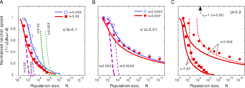
Figure 5: Normalized ratchet speed as a function of population size: analytic results versus simulation. Symbols correspond to simulation results, and lines correspond to theoretical predictions. The simulation results were obtained as described (Rouzine et al., 2003). Beneficial mutations are absent ($\alpha=0$). (A) Results for $\sigma=s/U=0.1$. The solid blue and red lines follow from the present work, Eq. (36). The dotted green lines follow from Gordo and Charlesworth (2000a), Eqs. (3a) and (3b). The dashed purple lines follow from Lande (1998), Eq. (2c) times $NU$. Parameters are shown. (B) As (A), but for $\sigma=s/U=0.01$. The dashed purple lines follow again from Lande (1998); the equivalent of the green lines in (A) falls outside of the axis range. (C) Effect of discreteness correction. The red squares and circles are identical to those in (A) and (B). The solid lines correspond to the prediction of traveling-wave theory without the discreteness correction, i.e., without a factor of $\sigma$ inside of the logarithm on the left-hand-side of Eq. (36), and without the denominator $1-v\ln(e/v)+5\sigma/6$ inside the logarithm on the right-hand side of Eq. (36). The dashed lines correspond to Eq. (36) without the entire second term on the right-hand-side. The arrow shows the value of $N$ at which the size of the least-loaded class $n_{0}=Ne^{-U/s}$ (Haigh, 1978) in the equilibrium distribution is 1 (at $s/U=0.1$).

This expression relates the selection strength $\sigma=s/U$, population size $N$, and mutation rate $U$ to the normalized ratchet rate, $v=(1/U)dk_{\text{av}}/dt$. We can evaluate this expression in two ways. First, we can assume the point of view that Eq. (36) describes $N$ as a function of $v$ and model parameters. Thus, we can directly plot $N$ over the entire range of $v$ ($0<v<1$). The solid lines in Fig. 5 were generated in this way. Alternatively, we can solve Eq. (36) numerically for $v$ at a given value of $N$.

We note that, at very small $\sigma$ and large $N$, the second term in the right- hand side of Eq. (36), originating from the stochastic edge treatment and the correction for discontinuity, can be neglected. In this limit, the substitution rate normalized to the mutation rate is expressed in terms of a single composite parameter $\sigma\ln(NU\sigma^{3/2})$. When this parameter is equal to 1, the ratchet rate, in this limit, becomes exactly zero. In fact, the ratchet speed is predicted (Gordo and Charlesworth, 2000a) to be finite albeit exponentially small at $\sigma\ln(NU\sigma^{3/2})>1$, when loss of the fittest genotype occurs so infrequently that the solitary wave approach breaks down (see below). At realistically small $\sigma$, the second term in Eq. (36) is important, as we show below by simulation, especially near $v=1$, where the first term vanishes as $(1-v)^{3}$, and at very small $v$, where the second term smears out the critical point $\sigma\ln(NU\sigma^{3/2})=1$.

The selection coefficient $s$ enters Eq. (36) through its rescaled version $\sigma=s/U$. Likewise, the ratchet speed $-V=dk_{\rm av}/dt$ enters in the rescaled form, $v=-V/U$. On first glance, this scaling looks unusual in comparison to the standard diffusion limit. In this limit, all results are expressed in terms of time rescaled with the population size, $t^{\prime}=t/N$ (Ewens, 2004), and rescaled mutation rate and selection coefficient, $U^{\prime}=NU$ and $s^{\prime}=Ns$. However, it is straightforward to express Eq. (36) in terms of the standard diffusion limit scaling. Note that a rescaling of time with $N$ means that we also have to rescale the ratchet rate, $V^{\prime}=NV$, and note further that $v=-V/U=-V^{\prime}/U^{\prime}$ and $\sigma=s/U=s^{\prime}/U^{\prime}$. Hence, if we replace the factor $NU$ on the left-hand side of Eq. (36) with $U^{\prime}$, Eq. (36) is given entirely in terms of the rescaled quantities of the standard diffusion limit, $V^{\prime},\ s^{\prime}$ and $U^{\prime}$.

3.3 Comparison with simulation results and other studies

We carried out simulations of Muller’s ratchet as described (Rouzine et al., 2003), and compared the measured ratchet speed to the speed predicted by Eq. (36) (Fig. 5). As shown previously (Rouzine et al., 2003), the traveling-wave theory leads to accurate predictions of the ratchet rate over a wide range of population sizes. Even though the theory is derived under the assumption that $N$ is large, we find that our prediction for the ratchet rate is accurate already for population sizes as small as $N=10$, and continues to be accurate throughout the entire range of biologically reasonable population sizes, until $\sigma\ln(NU\sigma^{3/2})$ becomes larger than 1. Thus, our results connect expressions for the ratchet rate derived by Lande (1998) or Gordo and Charlesworth (2000a) that work, respectively, for either very small or very large population sizes.

The transition to the regime of large $N$ occurs when the size of the least-loaded class is large, $N\exp(-1/\sigma)\gg 1$ (Gordo and Charlesworth, 2000a) (Fig. 5c). Then, clicks of the ratchet are rare, and the population is at equilibrium most of time. In contrast, in the intermediate interval of $N$ we study, the least-loaded class is not sufficiently large and is frequently lost. Therefore, a population does not have time to equilibrate between clicks. The non-equilibrium nature of the ratchet is witnessed by an almost constant, non-zero effective selection coefficient of the least-loaded class, $S>0$ and the fact that the width of the distribution is smaller than the equilibrium width, $\sqrt{\text{Var}[k]}<\sqrt{U/s}$, Eq. (11). The transition to the regime of small $N$ (Lande, 1998) occurs at $Ns\sim 1$, when fixation events of deleterious mutations at different sites are separated in time, and one-site theory applies.

We found that the term correcting for the discontinuity at $k=k_{0}$, Eq. (35), substantially improved the agreement between the numerical simulations and the analytical prediction of the ratchet speed for a large interval of population sizes (Fig. 5C). While the traveling-wave approximation (based on continuous treatment of fitness classes) combined with the stochastic treatment of the highest-fitness class is good enough to make useful predictions about the speed of Muller’s ratchet, the discreteness correction is necessary to achieve high prediction accuracy. The correction term becomes irrelevant only for very large population sizes, where the ratchet speed is dominated by the first term on the right-hand side of Eq. (36) (Fig. 5C, dashed lines).

Note that Rouzine et al. (2003) also used a correction term to account for the discontinuity at $k=k_{0}$. However, their term was obtained by fitting an interpolation formula to the numerical solution of Eqs.  (32) and (33). By contrast, here we derived the correction term analytically, as the asymptotic behavior near the high-fitness edge of the wave.

4 Speed of adaptation

If a population experiences a sudden change in environmental conditions or is introduced into a new environment, it will initially be ill-adapted. Over time, the population will accumulate beneficial mutations until a new mutation-selection balance is reached. The process of accumulating beneficial mutations is called positive adaptation, and the rate at which fitness changes over time is the speed of adaptation.

In our model, in the case of positive adaptation the speed of the wave is negative, $v<0$, because the wave moves towards smaller mutation numbers $k$. Furthermore, we make the assumption that we are far from mutation–selection balance, $|v|\gg 1$, i.e., $|dk_{\text{av}}/dt|\gg U$. In this regime, the rate of deleterious mutations is a small correction that can be neglected, and only the beneficial mutation rate affects our results. Therefore, it is more convenient to introduce, instead of $v$, the average substitution rate of beneficial mutations $V$, as given by

$$V=-\frac{dk_{\text{av}}(t)}{dt}=-Uv,$$ (37)

and the beneficial mutation rate $U_{\text{b}}=\alpha U$. The derivation that follows applies if $s$ is much larger than $U_{b}$, and the population size is sufficiently large, so that $V\gg s/\ln(s/U_{b})$. The latter condition ensures that the high-fitness tail of the distribution is long and the whole approach is valid. Within this validity region, we will consider two cases: moderate substitution rates, $s/\ln(s/U_{b})\ll V\ll s$, where the half-width of the fitness distribution is small, and relatively high substitution rates, $V\gg s$, where the distribution is broad.

4.1 Solitary wave approach in the adaptation limit

We expand $u$, $x_{0}$, $\phi^{\prime}(x_{0})$ [Eqs. (13) and (14)] and the right-hand side of Eq. (17) for large negative $v$ (dropping all terms small compared to $|v|$), and find

$$u =\frac{V}{U_{\text{b}}}\,,\quad\phi^{\prime}(x_{0})=\ln u=\ln\frac{V}{U_{\text{b}}}\,,$$ (38)

$$x_{0} =-\frac{V}{s}\Big{(}\ln\frac{V}{U_{\text{b}}}-1\Big{)}\,,$$ (39)

and

$$\phi(0)-\phi(x_{0})=\frac{V}{2s}\Big{(}\ln^{2}\frac{V}{eU_{\text{b}}}+1\Big{)}\,.$$ (40)

The approach rests on smoothness of $\ln f_{k}$. We obtain the continuity condition for $\ln f_{k}$ as before from Eq. (31), using $\phi^{\prime}\sim\ln u=\ln(V/U_{\text{b}})$ and Eq. (12). In Eq. (12), we keep only the third term in brackets: the first term is small, and the second term is important only near the edge. The resulting condition, $V\gg s/\ln(V/U_{\text{b}})$, is equivalent to $|x_{0}|\gg 1$. Just as in the case of Muller’s ratchet, the high-fitness tail must be long for our approach to work (Simplification 4).

Unlike in the ratchet case, even though the high-fitness tail is long, the half-width of the wave is not necessarily large. Large adaptation rates (large population sizes) correspond to a broad distribution, $\text{Var}[k]\gg 1$, and intermediate adaptation rates (intermediate population sizes) correspond to a narrow distribution, $\text{Var}[k]\ll 1$. For the two respective cases, from Eqs. (10) and (7) with $V\gg U$ ($v<0,|v|\gg 1$), we obtain

$$\phi(0) = -\frac{1}{2}\ln\frac{2\pi V}{s},\ \ V\gg s$$ (41)

$$\phi(0) = 0,\ \ s/\ln(V/U_{\text{b}})\ll V\ll s.$$ (42)

Again, we have to couple the deterministic wave equation to the stochastic behavior of the least-loaded class following the approach in Section 2.7. The condition that only the best-fit class should be treated stochastically reads $V\gg U_{b}$, which is equivalent to $s|x_{0}|\gg U_{b}$ (Simplification 7 and the end of this subsection).

Far above the stochastic threshold, the dynamics of the least-loaded class follows Eq.(18) with the effective selection coefficient $S$ and the mutation term $M$ given by

$$S=U+sx_{0}\approx-V\ln(V/U_{\text{b}}),\ \ M=U_{\text{b}}f_{k_{0}+1}.$$ (43)

Thus, the effective selection coefficient is negative, causing exponential expansion of the class. Unlike in the ratchet case, beneficial mutation events cannot be neglected: Their role is to add more and more clones to the class, resulting in a time-dependent prefactor influencing the growth of the class on large time scales. However, the logarithmic derivative of that growth is primarily determined by selection alone. To demonstrate the validity of this statement, we evaluate the relative magnitude of the two terms $M$ and $Sf_{k_{0}}$ in Eq.(18). From Eq. (43), we have

$$\frac{|S|f_{k_{0}}}{M}=\frac{V\ln(V/U_{\text{b}})}{U_{\text{b}}}\frac{f_{k_{0}}}{f_{k_{0}+1}}\,.$$ (44)

According to our continuous approximation, $\ln(f_{k_{0}+1}/f_{k_{0}})=\partial\ln f_{k_{0}}/\partial k_{0}=\phi^{\prime}(x_{0}).$ Thus, with $\phi^{\prime}(x_{0})=\ln(V/U_{\text{b}})$ [Eq. (38)], we find

$$\frac{|S|f_{k_{0}}}{M}=\ln\frac{V}{U_{\text{b}}}\gg 1\,.$$ (45)

Therefore, we can safely neglect the mutation term $M$ in the log-derivative of $f_{k_{0}}$ in time and approximate it with $|S|$, which fact will be used in the derivation below.

The dynamics of the current least-loaded class $f_{k_{0}}(t)$ above the stochastic threshold $1/(N|S|)$ represents a periodic saw-shaped dependence (Fig. 6). When beneficial mutations occurring in the least-loaded class generate a new least-loaded class with a size on the order of the stochastic threshold, with probability on the order of $1$, the new class will survive random drift and be further amplified by selection. We refer to this event as ”a class is established”. After a class is established, the wave moves one notch in $k$. By definition, the time period between establishment of two consecutive classes is given by $t_{\rm period}=1/V$. Below we estimate the size of the best-fit class $f_{\rm max}\equiv f_{k_{0}}(t_{\rm period})$ at the moment it gives rise to a new established class.

The total number of mutational opportunities (number of genomes that may potentially generate a beneficial mutation during one click) is $N$ multiplied by the time integral of $f_{k_{0}}(t)$ over one period, which is $Nf_{\rm max}/|S|$. In other words, because of the exponential growth of $f_{k_{0}}(t)$, most of the mutational opportunities will arise in a short time interval of length $1/|S|$ around the time when $f_{k_{0}}(t)$ has come close to the value $f_{\rm max}$ (Fig. 6). We note that that time interval is much shorter than the time of one click, $1/|S|=(1/V)/\ln(V/U_{\text{b}})\ll 1/V$. We obtain the average number of new least-loaded genomes created during one period by multiplying the number of mutational opportunities by the beneficial mutation rate $U_{\text{b}}$. Finally, each of these beneficial mutations have a probability $2|S|$ to survive drift (Haldane, 1927; Kimura, 1962). Therefore, the total number of beneficial mutations that arise and go to fixation during one period is $2|S|U_{\text{b}}Nf_{\rm max}/|S|=2U_{\text{b}}Nf_{\rm max}$. We find the desired value of $f_{\rm max}$ from the condition that, on the average, one new fitness class is established, which yields

$$f_{\rm max}\approx\frac{1}{2NU_{\text{b}}}\,.$$ (46)

Based on Fig. 6 and Eq.(46), we can also estimate the time of one click $1/V$ in terms of $S=sx_{0}$, as given by

$$\frac{1}{V}=\ln f_{\rm max}-\ln\frac{1}{N|S|}=\frac{1}{|S|}\ln\frac{|S|}{U_{b}}$$ (47)

which is similar to the expression $1/V=(1/|S|)\ln[V/(eU_{b})]$ obtained from the deterministic part of our derivation, Eq. (39). The difference is in the logarithmic factor $|S|/V\sim\ln(V/U_{b})$ in the argument of the large logarithm in Eq. (47). At the moment, we do not understand the discrepancy. The fact that $V$ as a function of $|x_{0}|$ can be obtained from considering either the stochastic edge (Desai and Fisher, 2007; Brunet et al., 2007) or the deterministic ”bulk” is certainly not trivial and deserves further inquiry.

The above estimate of $f_{\rm max}$ operates with fitness classes and does not depend on the particular clone composition of a class. Still, for the sake of clarity, we would like to make a comment on the clone composition of the least-loaded class. The estimate of $f_{\rm max}$ (defined within the accuracy of a numeric factor on the order of 1) corresponds to the short interval of time $\sim 1/|S|$ when a new least-loaded class is in the vicinity of the stochastic threshold, $f_{k_{0}}\sim 1/(N|S|)$ (Kimura and Ohta, 1973; Barton, 1995; Rouzine et al., 2001). At that time, the new class is comprised of a small number of clones (most likely, one or two). Later, as the next-loaded class increases nearly exponentially in time above $f_{\rm max}$, it generates additional clones joining the least-loaded class. Because the additional clones cross the stochastic threshold later than the first clone(s), they are consecutively smaller in size. As a result, the growing class consists of an increasing number of clones with decreasing relative sizes. However, the eventual clone composition of the best-fit class does not influence the estimate of $f_{\rm max}$, because it is formed at later times.

Now, following our general approach, Eq. (19), we match $\phi(x_{0})$ to the average between the minimum and the maximum value of $f_{k}(t)$ under deterministic growth (Fig. 6),

$$\phi(x_{0}) =\frac{1}{2}\Big{(}\ln f_{\max}+\ln\frac{1}{|S|N}\Big{)}$$

$$\approx-\ln\Big{[}N\sqrt{VU_{\text{b}}\ln(V/U_{\text{b}})}\Big{]}\,.$$ (48)

In comparison to the previous result by Rouzine et al. (2003) who matched $\phi(x_{0})$ directly to the stochastic threshold, the result found with the improved treatment of the stochastic edge differs by a factor of $\sqrt{(V/U_{\text{b}})/\ln^{3}(V/U_{\text{b}})}$ multiplying $N$.

As in the case of Muller’s ratchet, we can calculate a correction to the continuous approach that accounts for the deterministic perturbation of the wave shape caused by the discreteness of fitness class near $k=k_{0}$. The calculation is similar to the one for Muller’s ratchet, and the details are given in the appendix. The final expression for this correction term, Eq. (98), reads

$$\ln\left[2(k-k_{0})+1+{\cal O}\Big{(}\frac{1}{\ln(V/U_{\text{b}})}\Big{)}\right]\,.$$ (49)

We now replace $k-k_{0}$ by $|x_{0}|$, and neglect the term $+1$ in the above expression and the term $-Vs$ in $|x_{0}|$ [Eq. (39)], using the strong inequality $\ln(V/U_{\text{b}})\gg 1$. Then, the correction term becomes

$$\ln\left(\frac{V}{s}\ln\frac{V}{U_{\text{b}}}\right)\,.$$ (50)

Inserting Eqs. (4.1) and (41) into Eq. (40), adding the correction term (50) to the right-hand side of Eq. (40), and dropping all numerical constants multiplying $N$ inside the large logarithm, we arrive at our final result for large $V$,

$$\ln N\approx\frac{V}{2s}\Big{(}\ln^{2}\frac{V}{eU_{\text{b}}}+1\Big{)}-\ln\sqrt{\frac{s^{3}U_{\text{b}}}{V^{2}\ln(V/U_{\text{b}})}}\,,\quad V\gg s\,.$$ (51)

For intermediate $V$, $\phi(0)=0$ from Eq. (42), and the final result reads

$$\ln N\approx\frac{V}{2s}\Big{(}\ln^{2}\frac{V}{eU_{\text{b}}}+1\Big{)}-\ln\sqrt{\frac{s^{2}U_{\text{b}}}{V\ln(V/U_{\text{b}})}}\,,\quad s/\ln(V/U_{\text{b}})\ll V\ll s\,.$$ (52)

The difference between these two results is a factor of $\sqrt{V/s}$ multiplying the large population size $N$. As we found in simulations, the numeric effect of that difference is quite modest in a very broad parameter range. As in the case of Muller’s ratchet, we can evaluate expressions (51) and (52) either by calculating $N$ as a function of $V$, or by numerically solving for $V$ at a given value of $N$.

As in the case of Muller’s ratchet, we can express Eqs. (51) and (52) in terms of variables encountered in the standard diffusion limit, $V^{\prime}=NV$, $s^{\prime}=Ns$, and $U_{\text{b}}^{\prime}=NU_{\text{b}}$. First, note that $V/s=V^{\prime}/s^{\prime}$ and $V/U_{\text{b}}=V^{\prime}/U_{\text{b}}^{\prime}$. Second, after subtracting $\ln N$ from both sides of Eqs. (51) and (52), we obtain exactly the diffusion limit scaling for the terms $\ln\sqrt{s^{3}U_{\text{b}}/V^{2}}$ and $\ln\sqrt{s^{2}U_{\text{b}}/V}$ on the right-hand sides of these two equations.

For extremely large $N$, we can obtain an explicit expression for $V$ from Eq. (51) through iteration. In zero approximation, we have $V\sim s$. We insert this value into the logarithms in Eq. (51), substitute the resulting expression again into Eq. (51), and then neglect all numeric constants and terms of the form $\ln(s/U_{\text{b}})$ inside of large logarithms. We also neglect $\ln N$ when it multiplies $N$ in the argument of a logarithm (because $N$ is assumed to be very large). We find, to the first order,

$$V\approx\frac{2s\ln(N\sqrt{sU_{\text{b}}})}{\ln^{2}[(s/U_{\text{b}})\ln(N\sqrt{sU_{\text{b}}})]}\,.$$ (53)

The main difference from the previous asymptotic result of Rouzine et al. (2003) is the factor $\sqrt{sU_{b}}$ instead of $U_{b}$ multiplying $N$. [Note that in the corresponding equation in (Rouzine et al., 2003), Eq. (33) in the Supplementary Text, the factor $U_{\text{b}}$ multiplying $N$ was accidentally omitted.]

We assumed that only the best-fit class should be treated stochastically and that the next-loaded class, $k=k_{0}-1$, can be treated deterministically. The validity condition can be found from the requirement that the average size of the next-best class is much larger than the size of the best-fit class, which is either on the order of or larger than then stochastic threshold. Indeed, in this case the random drift term in the diffusion equation for the next-loaded class can be neglected as compared to the selection term. The requirement also ensures that, when a best-fit class gives rise to a new best-fit class, the former is much higher than the stochastic threshold. The validity condition is $V\gg U_{b}$, which is equivalent to $s|x_{0}|\gg U_{b}$ (Simplification 7). Because we already assumed the strong inequality $V\gg U_{b}$ when deriving Eqs. (51), (52), and (53), the next-loaded class can safely be considered deterministic in the entire region where the results of this section apply. Thus, unlike in the case of Muller’s ratchet, where the approximation of a single stochastic class introduces an error corresponding to a numeric factor multiplying $N$, in the case of adaption, the approximation is asymptotically accurate.

4.2 Comparison with simulation results for the adaptation rate

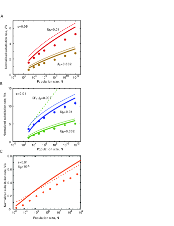
Figure 7: Normalized substitution rate as a function of population size, in the absence of deleterious mutations. Symbols correspond to simulation results, and thick solid lines correspond to analytic predictions obtained (A,B) from Eq. (51) or (C) from Eq. (52). Thin lines in (A,B) indicate the analytic prediction without discreteness correction, i.e., without term $\ln[(V/s)\ln(V/U_{\text{b}})]$ on the right-hand side of Eq. (51). Dotted lines in (B,C) indicate the analytic result by Desai and Fisher (2007), Eqs. 36, 38, and 39. Their result shown in (B) is outside of its designed validity range and is shown for reference only. The simulations were carried out (A,B) in discrete time as described (Rouzine et al., 2003) or (C) in continuous time. $V$ was measured in simulation as the average slope of $k_{\text{av}}(t)$ in the time interval $[0.85t_{0},1.15t_{0}]$, where the time $t_{0}$ of the interval center was determined from the condition $k_{\text{av}}(t_{0})=250$. The initial $k_{\text{av}}(0)$ was set to $1.5k_{\text{av}}(t_{0})$. The per-site beneficial mutation rate $\mu$ was chosen such that the genomic beneficial mutation rate $U_{\text{b}}$ had the value shown on the plot at time $t_{0}$, $U_{\text{b}}=\mu k_{\text{av}}(t_{0})$. The size of the symbols roughly corresponds to the largest standard deviation of the mean speed estimates.

We carried out simulations of adaptive evolution as described (Rouzine et al., 2003), and compared the measured speed of adaptation to the speed predicted by Eq. (51) in a wide range of parameter settings (Fig. 7A-C). Because deleterious mutations can be neglected in the limit $V\gg U$ we consider, the simulation results we present here were obtained in the absence of deleterious mutations, $U=U_{\text{b}}$, whereas Rouzine et al. (2003) considered beneficial and deleterious mutations at the same time.

Without the discreteness correction, Eq. (49), the analytic prediction of the wave speed generally follows the simulation results fairly well in a broad parameter range. The analytic result consistently overestimates the simulation result by 15 to 25% (Fig. 7A to C, dashed line). When we include the discreteness correction, the accuracy improves significantly across all parameter settings. In general, the accuracy becomes higher as $U_{\text{b}}$ and $s$ decrease. (If deleterious mutations are present, $U>U_{\text{b}}$, the predictions from traveling wave theory are at least as accurate—if not more so—as in the absence of deleterious mutations; see Fig. 2f in Rouzine et al. (2003) ).

For comparison, we show analytic results for the substitution rate obtained by Desai and Fisher (2007) who used a different approach [Eqs. (36), (38), and (39) in the cited work]. Their method applies at small adaptation rates where the lead $|x_{0}|$ is only moderately large (see our Discussion). In its validity range, the prediction is very similar to ours (Fig. 7C, dotted line). Note that Desai and Fisher (2007) in their Fig. 5 compare with simulation not the actual analytic result, but its simplified version, Eq. (41), which accidentally gives a higher accuracy than the actual result. When the lead is large and the approach breaks down, their analytic prediction is far from simulation results (Fig. 7B, dotted line).

4.3 Testing stochastic edge treatment: Simulation of a two-class model

In order to validate our results and to get further insight into the dynamics of the stochastic best-fit class, we carried out a computer simulation for a simplified model including only two fitness classes, the best-fit class, and the second-best class (Desai and Fisher, 2007) . Only the best-fit class was treated stochastically. The aim was to confirm the analytic estimate of the size of the second-best class when the new best class is established, Eq. (46). The way it was derived, the estimate is expected to be robust with respect to such a model simplification. Note that the two-class model cannot be used to test other intermediate results of this section.

According to the two-class model, we assume that the frequency of the second-best class grows as

$$f_{k_{0}-1}(t)=\frac{1}{Ns|x_{0}|}e^{s(|x_{0}|-1)t},$$ (54)

where $1/(s|x_{0}|)$ is the characteristic size where selection prevails over genetic drift. (In other words, we ignore stochastic effects and mutants coming from less-fit classes.) According to the main model, the average frequency of the best class grows as

$$f_{k_{0}}(t+1)=e^{s|x_{0}|}f_{k_{0}}(t)+U_{\text{b}}f_{k_{0}-1}(t)=e^{s|x_{0}|}f_{k_{0}}(t)+\frac{U_{\text{b}}}{Ns|x_{0}|}e^{s(|x_{0}|-1)t}.$$ (55)

In our pseudorandom simulation, we calculated the actual size of the best class $Nf_{k_{0}}(t)$ over a long time scale using Poisson statistics with the average given by Eq. (55). Then, to find the time delay between the growth of two classes, we extrapolated $f_{k_{0}}(t)$ back from large times $t\gg 1/s|x_{0}|$ when the best-fit class was large enough to be treated deterministically, $Nf_{k_{0}}\gg 1/s|x_{0}|$, as follows.

We seek a solution of Eq. (55) in the form $f_{k_{0}}(t)=A(t)e^{s|x_{0}|t}$. Inserting this expression into Eq. (55) and solving the equation in discrete time with respect to $A(t)$, we obtain

$$f_{k_{0}}(t)=e^{s|x_{0}|t}\left[A(0)+\frac{U_{\text{b}}e^{-s|x_{0}|}}{s|x_{0}|}\frac{1-e^{-st}}{1-e^{-s}}\right],$$ (56)

where $A(0)$ is an arbitrary constant. Strictly speaking, $A(0)$ is random and has to be found from the stochastic edge simulation.

Instead of $A(0)$, we introduce a more transparent parameter, the time delay between establishment of two consecutive best-fit classes $\tau$, as given by the periodicity condition

$$f_{k_{0}}(\tau)=f_{k_{0}-1}(0)=\frac{1}{Ns|x_{0}|}.$$ (57)

From Eq. (56), the parameter $\tau$ is related to $A(0)$ as given by

$$A(0)=\frac{1}{s|x_{0}|}\left[{e^{-s|x_{0}|\tau}+U_{\text{b}}e^{-s|x_{0}|}\frac{e^{-s\tau}-1}{1-e^{-s}}}\right].$$ (58)

In terms of $\tau$, the growth curve of the best-fit class, Eq. (56), can be written as

$$f_{k_{0}}(t)=\frac{1}{Ns|x_{0}|}e^{s|x_{0}|t}\left[{e^{-s|x_{0}|\tau}+U_{\text{b}}e^{-s|x_{0}|}\frac{e^{-s\tau}-e^{-st}}{1-e^{-s}}}\right].$$ (59)

We obtain $\tau$ by measuring $f_{k_{0}}(t)$ in simulation at some large time $t$, such that $t\gg 1/s|x_{0}|$, and then solving Eq. (59) numerically for $\tau$. We checked that changing the sampling time $t$ within the range $\tau$ to $10\tau$ has a small effect on the result for $\tau$, which confirms the vadity of our back-extrapolation procedure.

Finally, in order to test the accuracy of our analytic estimate, Eq. (46), we calculate the constant $C$ in the stochastic edge simulation, as given by

$$C=NU_{\text{b}}f_{k_{0}-1}(\tau)\equiv NU_{\text{b}}f_{\rm max}.$$ (60)

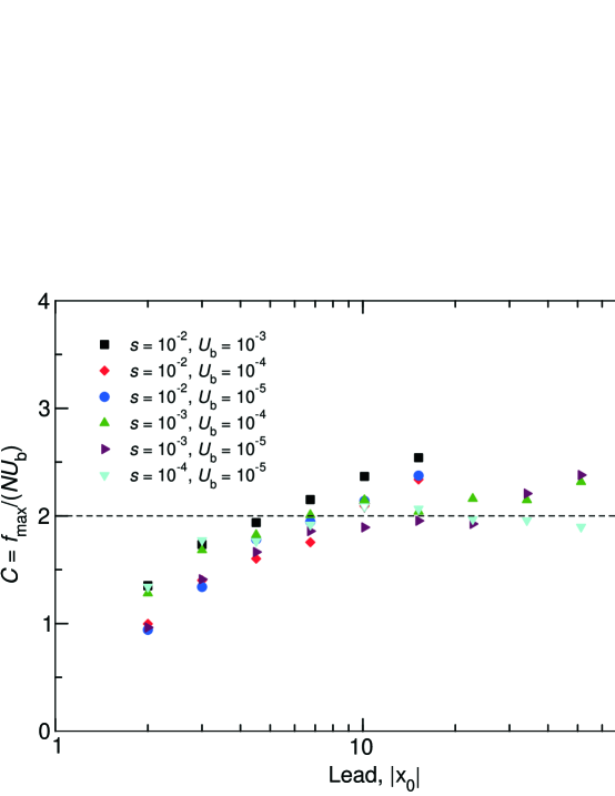
Figure 8: Test of the accuracy of the stochastic edge treatment, Eq. (46). Points are obtained by simulation using a simplified two-class model. Only points corresponding to $s|x_{0}|<0.2$ are shown. Parameter values are shown.

We averaged the value of $\log C$ over 500 simulation runs. The result is shown in Fig. 8 for various values of $|x_{0}|,s$, and $U_{b}$. In principle, the analytic result that $C=\text{const}\approx 2$ is supposed to be asymptotically correct at $|x_{0}|\gg 1,s|x_{0}|\ll 1$. In the parameter region $|x_{0}|>5$ and $s|x_{0}|<0.2$, the value of $C$ varies between 1.5 and 2.5 . (Note that even though Eq. (60) seems to imply that $C$ depends on $N$, this factor actually cancels.) Because $C$ is only a numeric factor at $N$, and $N$ is large and enters a logarithm in the expression for the substitution rate, such variation of $C$ has a small effect on the final substitution rate and thus confirms the validity of our analytic estimate, Eq. (46).

It is important that, due to constant influx of new beneficial mutants from the second-best class, the best-fit class size does not grow exactly exponentially, Eq. (59). We checked that replacing Eq. (59) with an exact exponential in the back-extrapolation procedure seriously affects the result for $\tau$ and makes it depend on the (arbitrarily chosen) sampling time $t$ (results not shown). This facts explains why the approach by Desai and Fisher (2007), who used the exponential back-extrapolation to estimate $\tau$, works only at very small adaptation rates when $|x_{0}|\sim 1$ [Fig.  7) (see Discussion and Brunet et al. (2007)].

4.4 Crossing over to the single site model

We expect intuitively that, for extremely large population sizes, the speed of adaptation should cross over to its deterministic, infinite-population-size behavior. In the deterministic limit, the process of creation and fixation of rare mutants does not affect the speed of adaptation, because all possible mutants are instantaneously present. Instead, the speed of adaptation depends simply on the growth rate of the mutants at different sites. As a consequence, in the mulitplicative fitness model, linkage between sites becomes irrelevant, and we can describe the system behavior with the single site model,

$$\frac{df}{dt}=sf(1-f)+\mu_{\text{b}}(1-f)\,,$$ (61)

where $f$ is the frequency of the beneficial allele at the given site, and we have assumed that deleterious mutations do not occur. The time it takes for a beneficial clone to grow from size 0 to size $f_{0}$ is $T=\ln[(sf_{0}+\mu_{\text{b}})/(\mu_{\text{b}}-f_{0}\mu_{\text{b}})]/(s+\mu_{\text{b}})$. Setting $f_{0}=1/2$ and assuming $s\gg\mu_{\text{b}}$, we find that the half-time of reversion, in which the beneficial clone grows to 50% presence, is

$$T_{1/2}\approx(1/s)\ln(s/\mu_{\text{b}})\,.$$ (62)

The same equation applies to a population of genomes that contain multiple sites which are independent and unlinked. Thus, if at some time point there are $k_{\text{av}}$ deleterious alleles fixed in the population, then Eq.  (62) gives the time interval until, on average, all members of the population have reverted half of these deleterious alleles.

To test our intuitive expectation, we will now compare this expression to the corresponding expression from traveling wave theory. For a wave centered at position $k_{\text{av}}$, the time to revert half of the deleterious mutations is

$$T_{1/2}\approx\frac{k_{\text{av}}}{2V}\,.$$ (63)

After inserting Eq. (53) into Eq.  (63) and keeping only the leading terms in $N$, we find that at $\ln N\sim k_{\text{av}}\ln(s/\mu_{\text{b}})$, the half-time of reversion crosses over to the single-site expression Eq. (62) (under the assumption that $s\gg\mu_{\text{b}}$). The reason for this behavior is that once $\ln N$ grows to $k_{\text{av}}\ln(s/\mu_{\text{b}})$, the left edge of the wave reaches the mutation-free genome. At this point, the assumption $k_{\text{av}}\gg k_{\text{av}}-k_{0}$ is violated, and the traveling-wave approach ceases to be valid. For population sizes exceeding $k_{\text{av}}\ln(s/\mu_{\text{b}})$, the system behavior is essentially independent of population size, and linkage does not slow down the speed of adaptation.

5 Discussion

We have derived accurate expressions for the speed of Muller’s ratchet and the speed of adaptation in a finite, asexual population. Our expressions are numerically valid in a wide parameter range. The main difference between the work presented here and the work of Rouzine et al. (2003) is an improved and more intuitive treatment of the stochastic egde, and the analytic derivation of correction terms for the discontiuity at $k=k_{0}$ for both Muller’s ratchet and the speed of adaptation. The latter correction terms lead to significantly improved numerical accuracy in a wide range of population sizes.

5.1 Muller’s ratchet

A quantitative treatment of Muller’s ratchet was first attempted by Haigh (1978), who studied primarily the case in which ratchet clicks are rare, so that the population can equilibrate between subsequent ratchet clicks. Since then, numerous studies have derived improved estimates of the ratchet rate (Pamilo et al., 1987; Stephan et al., 1993; Gessler, 1995; Higgs and Woodcock, 1995; Prügel-Bennett, 1997; Lande, 1998; Gordo and Charlesworth, 2000a, b). Most approaches to calculate the ratchet rate work either in the case $N<1/s$, when fixation events of deleterious alleles at different sites are well separated in time and the one-site theory applies, or in the limit of very large population sizes, when the deterministic expectation for the size of the fittest class $n_{0}=N\exp(-U/s)$ is much larger than 1. In the former case, the ratchet rate is estimated as the rate at which deleterious mutations enter the population, multiplied with the probability of fixation of deleterious mutations (Lande, 1998). In the latter case, the ratchet rate is estimated from the average time the fittest class takes to drift from its equilibrium value to an occupancy of zero (Stephan et al., 1993; Gordo and Charlesworth, 2000a, b). A third approach, most closely related to the present work, is a quantitative genetics approach whereby the fitness distribution is described by its mean, variance, and higher moments, and equations are derived that describe the change of these moments over time (Pamilo et al., 1987; Higgs and Woodcock, 1995; Prügel-Bennett, 1997). A disadvantage of this approach is that it generally requires an arbitrary cutoff condition to truncate the moment expansion, and that the equations become quickly untractable if higher moments are included.

The rapid ratchet region described in the present work corresponds, mostly, to $n_{0}$ smaller than 1 (Fig. 5c). For small $n_{0}$, the work by Gessler (1995) is generally regarded as giving accurate estimates for the ratchet rate. However, it is important to emphasize that Gessler (1995) did not actually derive a closed form expression for the ratchet rate. A key parameter in his result needs to be determined numerically by iteration. Moreover, several of his expressions were not derived from first principles, but chosen on the basis that they provided a good fit to simulation results. In contrast, our expression Eq. (36) was derived from first principles and is a simple, closed-form expression that can be plotted easily, if we interpret it as describing $N$ as a function of $v$ (rather than $v$ as a function of $N$).

The traveling wave approach also provides a convenient framework to study the ratchet speed in the presence of beneficial mutations, or, conversely, the speed of adaptation in the presence of deleterious mutations. All that is required is to keep the full expression $\phi(0)-\phi(x_{0})$, Eq. (17), instead of its respective asymptotics. While we did not discuss these cases here in detail, the corresponding calculations are straightforward and lead to closed-form expressions [see (Rouzine et al., 2003), Supplementary Text]. In comparison, other approaches may lead to similarly accurate expressions, but usually do not yield closed-form expressions. For example, Bachtrog and Gordo (2004) studied the effect of beneficial mutations in the presence of Muller’s ratchet. They used a Poisson approximation for the steady-state distributions of mutations in populations undergoing Muller’s ratchet, explicitly modeled the behavior of beneficial mutations arising in all possible mutation classes, and used the resulting fixation rates as corrections for the ratchet rate derived by Gessler (1995) for $n_{0}<1$ and by Gordo and Charlesworth (2000a, b) for $n_{0}>1$. This approach leads to accurate results in a wide parameter range, but the final equations contain sums over all mutation classes, and these sums cannot be evaluated analytically.

Finally, with the traveling wave approach, it is also possible to consider the general case when both beneficial and deleterious mutations are equally important, including steady state at finite $N$, $v=0$ in Eq. (17), which differs from equilibrium at infinite $N$ (Rouzine et al., 2003). However, to achieve a high accuracy in this case requires some additional work on the stochastic edge condition.

5.2 Adaptation

In an asexual population, the speed of adaptation does not grow linearly with $N$ for large $N$, because beneficial mutations that arise contemporaneously in independent genetic backgrounds cannot recombine, and, therefore, only a small fraction of all beneficial mutations that survive drift can actually go to fixation (Fisher, 1930; Muller, 1932; Crow and Kimura, 1965; Hill and Robertson, 1966; Maynard Smith, 1971). One reason why a beneficial mutation may not go to fixation is interference with another mutation with a larger beneficial effect that arises either shortly before or shortly after the first mutation (Barton, 1995). Recently, a theory that predicts the evolutionary rate in large asexual populations in the presence of this interference process has received considerable attention (clonal interference-theory, Gerrish and Lenski, 1998; Orr, 2000; Wilke, 2004). However, interference does not necessarily occur in the presence of a single alternative mutation. In fact, multiple beneficial mutations arising in the already existing clones — that have moderate individual effect but large combined effect—can rescue clones with a smaller beneficial effect and partly resolve the clonal interference. The clonal interference theory neglects this effect and predicts that the substitution rate rapidly approaches a constant with increasing $N$ (under the assumption of exponentially distributed beneficial effects, Wilke, 2004), and that further increases in the speed of adpatation can only come from fixation of mutations with increasingly larger beneficial effects. This prediction is, most likely, not entirely correct, because an increase in population size also increases the chance that multiple mutations occur in the same clone. In general, we expect the clonal interference theory to have a very limited range of applicability. If beneficial mutations are rare, interference is irrelevant to the speed of adaptation, and $V$ is proportional to $NU_{\text{b}}$. On the other hand, if the population size is large and beneficial mutations are frequent, then multiple mutations within a single clone should be frequent as well, and we expect the current clonal interference theory to underestimate the speed of adaptation in this regime.

In contrast to the clonal interference approach, the traveling wave approach considers multiple mutations. However, the present model does not consider interference from mutations with a larger beneficial effect, because all mutations are assumed to have the same selection coefficient. (Note that, as a consequence, the substitution rate and the speed of adaptation are essentially equivalent in our model, as they differ only by a constant factor $s$, whereas they are distinct quantities if there is variation in the selection coefficient, as is the case in the clonal interference models.) Because of these differences in model assumptions, we cannot make a quantitative comparison between the two theories. However, we can observe an important qualitative difference: in the traveling-wave theory, the substitution rate keeps slowly increasing with population size until extremely large population sizes.

For very large population sizes, such that $\ln N\sim k_{\text{av}}\ln(s/\mu_{\text{b}})$, the substitution rate becomes on the order of $sk_{\rm av}$. At this point, the tail of the wave reaches the best possible genome, $k=0$, and the traveling wave theory breaks down (Rouzine et al., 2003). At higher population sizes, the one-locus model applies, and the value of the substitution rate saturates at the infinite-size value. Thus, we predict a continuous transition from the finite-population case in which linkage slows down the speed of adaptation to the infinite-population case in which linkage has no effect on the speed of adaptation in the multiplicative model (Maynard Smith, 1968). By contrast, Maynard Smith (1971) argued that a finite asexual population is always affected by linkage, regardless of its size. We must mention, however, that, for reasonable parameter settings, the population size at which the crossing over to the fully deterministic behavior occurs is unbiologically large. For example, assuming $k_{\text{av}}=20$ and $s/\mu_{\text{b}}=1000$, we find that $N$ has to be on the order of $10^{60}$, and this number grows rapidly for larger $k_{\text{av}}$.

It is important to stress that the speed of adaptation is, in general, not governed by the total supply of beneficial mutations, $NU_{\text{b}}$, because $N$ and $U_{\text{b}}$ enter the expressions for the speed of adaptation independently and in different functional forms. This fact had already been noted by Maynard Smith (1971), and its implications for experimental tests of the speed of adapation have been discussed recently in the context of clonal interference theory (Wilke, 2004).

Recently, Desai and Fisher (2007) have proposed an alternative method to derive, for the same initial model, the speed of adaptation in a large asexual population in the absence of deleterious mutations. We discuss this method in detail and extend its validity range elsewhere (Brunet et al., 2007). Briefly, these authors replace the full population model with a simplified model including only two fitness classes, the least-loaded class and the next-loaded class. The next-loaded class is assumed to grow exactly exponentially, as if under selection alone. The click time $1/V$ is determined by extrapolating the growth of the least-loaded class back from infinite time. As in our work, only the least-loaded class is treated stochastically.

The main validity conditions for this approach are, as follows. The next-loaded class can be treated deterministically if $s|x_{0}|\gg U_{b}$, which is equivalent to $V\gg U_{b}$, the same condition that we use in our work. (Note that inequality $s\gg U_{b}$ given by Desai and Fisher (2007) was obtained for $|x_{0}|\sim 1$; for general $|x_{0}|$, the condition is as we state.) The back-extrapolation procedure is valid at moderate population sizes or adaptation rates, such that $\ln|x_{0}|\ll\ln(s/U_{b})$ (Brunet et al., 2007). A sufficient validity condition is $|x_{0}|\ll\ln(s/U_{b})$, which is equivalent to $V\ll s$ (note that the cited paper contains a typo in that condition; M. Desai, pers. comm.). The accuracy of the replacement of the full population model with the two-class model and of the actual dynamics of the next-loaded class with an exponential is less clear. New beneficial mutations into the class create a time-dependent prefactor at the exponential. Yet, it is quite possible, that at moderate $|x_{0}|$ or $V$ where the cited approach is designed to apply, the approximation works well. We tested the numeric accuracy of the substitution rate predicted by Desai and Fisher (2007) with the use of Monte-Carlo simulation of the full population model in different parameter regions. Within its validity range, their result agrees with simulation within 10-20% and is very similar to our result (Fig. 7C). [Note that the extremely high numeric accuracy shown in Fig. 5 of the cited work is due to replacement of the actual final result, Eq. (39), with its asymptotics for very large $N$, Eq. (40), which does not apply at such moderate $N$.]

In their Discussion section, Desai and Fisher (2007) state that the traveling wave approach Rouzine et al. (2003) requires that the fitness distribution is smooth in mutational load and, hence, broad, which takes place at large substitution rates, $V\gg s$. Proposing some estimates of parameter values of $U_{b}$ and $s$ typical for yeast, they argue that this regime corresponds to huge population sizes and conclude that results by Rouzine et al. (2003) are relevant for viruses only. In fact, the traveling wave approach requires that the logarithm of the fitness distribution, not the fitness distribution itself, is smooth in the mutational load, which takes place when the high-fitness tail of the distribution $|x_{0}|$ (not the half-width) is larger than 1. The condition is met at much smaller substitution rates, $V\gg s/\ln(V/U_{b})$, which is the low bound assumed by Desai and Fisher (2007). The likely reason for the confusion is that Rouzine et al. (2003) normalized the fitness distribution assuming it is broad, which corresponds to the case $V\gg s$. When the wave is narrow, which happens in the interval $s/\ln(V/U_{b})\ll V\ll s$, the normalization condition is simply replaced with $\phi(0)=0$ (Subsection 2.4). Except for the trivial change in normalization, whether the wave is broad or narrow does not matter. In the final expression for the substitution rate, the difference between the two cases $s/\ln(V/U_{b})\ll V\ll s$ and $V\gg s$ is in a constant factor at $N$, Eqs. (52) and (51). Numerically, the two expression are quite similar in the parameter range we test. Therefore, the results of the traveling wave approach apply in both intervals of the substitution rate and are potentially relevant for a broad variety of asexual organisms, including RNA and DNA viruses, yeast, coral, and some species of plants and fish.

To summarize, we have applied the semi-deterministic traveling wave approach to derive the rate of Muller’s ratchet and the speed of adaptation in a multi-site model of an asexually reproducing population. Our results underscore the importance of a proper stochastic treament of the best-fit class. Our method, based on a continuous approximation to logarithm of the fitness distribution of the other (deterministic) classes, ensures fair accuracy in a very broad parameter range. In addition, an analytic correction for the discreteness of fitness of the deterministic classes significantly increases the accuracy of predictions.

Appendix A Appendix

A.1 Main simplifications of the derivation

Below we list the main simplifications employed in the derivation of the traveling wave solution and determine parameter regions in which they are asymptotically correct. A brief summary of the validity conditions is as follows. The values of $s,U$, and $U_{b}$ are assumed to be much smaller than 1. The number of sites is large and the wave is far away from the two extremes of a mutation-free or a completely mutated genome, $L\gg 1,k_{\text{av}}\gg|x_{0}|,L-k_{\text{av}}\gg|x_{0}|$. Other conditions depend on the case.

For Muller’s ratchet, we assume $s\ll U\ll 1$ and $N\gg 1/(U\sigma^{2/3})$. These conditions ensure that the high-fitness tail is long. Also, for the ratchet to proceed rapidly and continuously rather than by exponentially rare clicks, we need $\ln(Ns^{3/2}U^{1/2})\ll U/s$ (Section 3.3).

For the adaptation regime, to have a single stochastic class, we assume $V\gg U_{b}$, which is equivalent to $U_{b}\ll s|x_{0}|$. To expand fitness in the mutational load, we assume $s|x_{0}|\ll 1$. We also need a long tail of the fitness distribution, $|x_{0}|\gg 1$. In terms of the substitution rate $V$, the last two conditions read $s/\ln(V/U_{b})\ll V\ll 1/\ln(1/U_{b})$. In terms of $N$, they read $N\gg\sqrt{s/U_{b}^{3}}/\ln(s/U_{b})$ and $\ln(N\sqrt{sU_{b}})\ll(1/s)\ln^{2}(1/U_{b})$.

Simplification 1: Linear selection term. We can expand $e^{-sx}$ as $1-sx$ under the condition $s|x|\ll 1$. In the case of Muller’s ratchet, we find from Eq. (21) that this condition is equivalent to $U\ll 1$. In the case of adaptive evolution, we find from Eq. (39) that this condition is equivalent to $V\ll 1/\ln(1/U_{b})$, which is met numerically in all cases we consider (Fig. 7) and analytically at $\ln(N\sqrt{sU_{b}})\ll(1/s)\ln^{2}(1/U_{b})$, Eq.(53).

Simplification 2: Distribution is far from the origin. Because $\alpha_{k}$ depends only slowly (linearly) on $k$, we are allowed to replace $\alpha_{k}$ by $\alpha\equiv\alpha_{k_{\text{av}}}$ under the condition that $L\gg 1$, $k_{\text{av}}\gg|x_{0}|$, $L-k_{\text{av}}\gg|x_{0}|$ (i.e., the wave is far away from the two extremes of a mutation-free or a completely mutated genome, and narrow in comparison to the average mutational load).

Simplification 3: Continuity in time. Approximating $f_{k}(t+1)/f_{k}(t)$ with $1+\partial\ln f_{k}(t)/\partial t$ is justified when $|\partial\ln f_{k}(t)/\partial t|\ll 1$. Replacing $|\partial t|$ and $\ln f_{k}(t)$ with $|dx/(vU)|$ and $\phi(x)$, respectively, we find that this condition takes the form $U|v\phi^{\prime}(x)|\ll 1$. Because $|\phi^{\prime}|$ increases with $|x|$, the far low- fitness tail is not very important for evolution, and in the high-fitness tail $|\phi^{\prime}(x)|<|\phi^{\prime}(x_{0})|$, the sufficient condition takes a form $U|v|\ln u\ll 1$, where $u$ is defined in Eq. (13).

In the ratchet limit, $\alpha=0$, after substituting $u$ from Eq. (20), the validity condition becomes $Uv\ln(1/v)\ll 1$, which is met at any $v$, $0<v<1$, as long as $U\ll 1$. Note that the condition is equivalent to $S\ll 1$, as in Simplification 1.

In the adaptation limit, where deleterious mutations can be neglected, the validity condition takes a form $V\ln(V/U_{b})\ll 1$, where $V\equiv-Uv$ and we used Eq. (38) for $u$. Again, the validity condition is $|S|\ll 1$, which is approximately equivalent to the condition $s|x_{0}|\ll 1$ we used to expand fitness in $k$ (Simplification 1).

For sufficiently (and unrealistically) large $N$, $V$ becomes large as well, and the condition $|S|\ll 1$ may be violated. In this region, technically, we can neither expand fitness in $k$ nor replace discrete time with continuous time (Simplifications 1 and 3 cannot be used). Nevertheless, Rouzine et al. (2003) showed that the continuous equation for the fitness distribution, Eq. (4), can be derived in a more general way, without assuming $|\partial\ln f_{k}(t)/\partial t|\ll 1$, nor expanding fitness in $k$, nor neglecting multiple mutations per genome per generation [see the transition from Eq. (1) to Eq. (11) in the Supplementary Text of the quoted work]. In the present work, we use these approximations to simplify our derivation.

Simplification 4: Continuity in $k$. Replacement of $\ln[f_{k+1}(t)/f_{k}(t)]$ with the partial derivative $\partial\ln f_{k}(t)/\partial k$ is justified if $|\partial\ln f_{k}/\partial k|\gg|\partial^{2}\ln f_{k}/\partial k^{2}|$. With $\partial\ln f_{k}/\partial k=\phi^{\prime}$, we can rewrite this condition as $|\phi^{\prime}|\,|dx/d\phi^{\prime}|\gg 1$. This condition is already discussed in the section on the continuity correction for Muller’s ratchet, and also in the section on the speed of adaptation, after Eq. (40). In short, this simplification is justified if the left tail is long, $|x_{0}|\gg 1$. Let us express this condition in terms of the substitution rate and $N$.

For Muller’s ratchet, based on Eq. (21), the condition $|x_{0}|\gg 1$ is met if $\sigma\ll 1$, and the ratchet rate is not to close to the maximum, $1-v\gg\sqrt{\sigma}$. The latter condition is always met, because the more limiting condition is that the wave tail is longer than the half-width, $|x_{0}|\gg\sqrt{{\rm Var}[k]}$, which is equivalent to the requirement $\phi(0)-\phi(x_{0})\gg 1$. In terms of $v$, that condition reads $1-v\gg\sigma^{1/3}$, Eqs. (23) and (21). The lower bound on $N$ follows from the final relation between $N$ and $v$, Eq. (36), which yields $N\gg 1/(U\sigma^{2/3})$.

For adaptation, the condition of a long high-fitness tail can be found from Eq. (39) for $|x_{0}|$, as given by $V\gg s/\ln(V/U_{b})\approx s/\ln(s/U_{b})$. The lower bound on $N$ follows from the final result for the adaptation speed, Eq. (52), as given by $N\gg\sqrt{s/U_{b}^{3}}/\ln(s/U_{b})$.

Simplification 5: Slow change of the wave shape. In the derivation of Eq. (6), we neglected any change in the wave shape over time, i.e., we assumed that $|\partial\phi/\partial t|\ll 1$. This condition is satisfied when the distribution is far from the origin, Simplification 2 [see (Rouzine et al., 2003), Supplementary Text, Approximation 6 for details].

Simplification 6: Broad and narrow wave. If the wave is broad, $\text{Var}[k]\gg 1$, to determine $\phi(0)$, we can expand $e^{\pm\phi^{\prime}(x)}$ near the wave center linearly as $1\pm\phi^{\prime}(x)$ if $|\phi^{\prime}(x)|\ll 1$. This condition is met for any $v$, whether positive or negative, if $\sigma\ll 1$ (i.e., $s\ll U$). If $\sigma$ is not small, the condition is is met at large negative $v$ (rapid adaptive evolution): $|v|\gg\sigma$ or $V\gg s$. In the opposite limit of narrow wave, we have $\text{Var}[k]\ll 1$, so that $\phi(x)$ is narrow and cannot be approximated by a Gaussian even near its center. In this case, we use instead $\phi(0)=1$. Together, these two limits cover the entire parameter range.

Simplification 7: Single stochastic class in the adaptation case. Now we verify the initial approximation that the next-loaded class, $k=k_{0}-1$, can be treated deterministically. The average ratio of its size to the least-loaded class size is given by $f_{k_{0}-1}/f_{k_{0}}=\exp[\phi^{\prime}(x_{0})]=u=V/U_{b}$, Eq. (38). Thus, the condition that only one class has to be treated deterministically is $V\gg U_{b}$. The strong inequality also ensures that, when a best-fit class gives rise to a new best-fit class, the former is much higher than the stochastic threshold, $f_{\rm max}\gg 1/(Ns|x_{0}|)$, Eqs.  (46) and (39).

A.2 Connection between the width and speed of the wave—alternative derivation

We derived the maximum ratchet rate ($v<1-2\alpha$) from the variance of $k$, Eq. (11), which in turn we derived from the normal approximation to the shape of the wave, Eq. (8). We can alternatively derive the same result directly from Eq. (3). We write $f_{k}(t+1)-f_{k}(t)=U\partial f_{k}(t)/\partial\tau$, multiply both sides of Eq. (3) with $(k-k_{\text{av}})/U$, and sum over all $k$. We find

$$\sum_{k}(k-k_{\text{av}})\frac{\partial f_{k}(t)}{\partial\tau} =(1-\alpha)\sum_{k}(k-k_{\text{av}})f_{k-1}(t)+\alpha\sum_{k}(k-k_{\text{av}})f_{k+1}(t)$$

$$\qquad\qquad-\sum_{k}(k-k_{\text{av}})[1+\sigma(k-k_{\text{av}})]f_{k}(t)\,.$$ (64)

The term on the left hand side of Eq. (A.2) evaluates to

$$\sum_{k}(k-k_{\text{av}})\frac{\partial f_{k}(t)}{\partial\tau} =\frac{\partial}{\partial\tau}\sum_{k}kf_{k}(t)-k_{\text{av}}\frac{\partial}{\partial\tau}\sum_{k}f_{k}(t)$$

$$=\frac{\partial k_{\text{av}}}{\partial\tau}=v\,.$$ (65)

The first term on the right-hand side of Eq. (A.2) evaluates to

$$(1-\alpha)\sum_{k}(k-k_{\text{av}})f_{k-1}(t) =(1-\alpha)\Big{[}\sum_{k}(k-1)f_{k-1}(t)+(1-k_{\text{av}})\sum_{k}f_{k-1}(t)\Big{]}$$

$$=(1-\alpha)\,.$$ (66)

Likewise,

$$\alpha\sum_{k}(k-k_{\text{av}})f_{k+1}(t)=-\alpha$$ (67)

and

$$\sum_{k}(k-k_{\text{av}})[1+\sigma(k-k_{\text{av}})]f_{k}(t)=\sigma\sum_{k}(k-k_{\text{av}})^{2}f_{k}(t)\,.$$ (68)

Since $\sum_{k}(k-k_{\text{av}})^{2}f_{k}(t)=\text{Var}[k]$, we find

$$v=1-2\alpha-\sigma\text{Var}[k]\,,$$ (69)

which corresponds to Eq. (11).

A.3 Correction to the continuity approximation for the case of Muller’s ratchet

We wish to compute the steady state proportions $f_{k}(t)$ from Eqs. (32) and (33), under the periodic boundary condition

$$f_{k-1}(0)=f_{k}[1/(Uv)]\,.$$ (70)

We introduce the generating function

$$G(\lambda,t)=\sum_{n\geq 0}f_{k_{0}+n}(t)\lambda^{n}.$$ (71)

From Eqs. (32) and (33), we obtain

$$\frac{\partial}{\partial t}G(\lambda,t)=-SG(\lambda,t)+U\lambda G(\lambda,t),$$ (72)

so that

$$G(\lambda,t)=G(\lambda,0)e^{(U\lambda-S)t}.$$ (73)

We find $G(\lambda,0)$ from Eq. (70) and Eq. (32)

$$G(\lambda,0) ={1\over\lambda}G\Big{(}\lambda,{1\over Uv}\Big{)}-{1\over\lambda}f_{k_{0}}\Big{(}{1\over Uv}\Big{)}$$

$$={1\over\lambda}e^{{U\lambda-S\over Uv}}G(\lambda,0)-{1\over\lambda}f_{k_{0}}(0)e^{-{S\over Uv}}.$$ (74)

Finally, using the fact that $S=Uv\ln(e/v)$, we find

$$G(\lambda,0)={f_{k_{0}}(0)\over e^{\lambda\over v}-\lambda e^{S\over Uv}}={f_{k_{0}}(0)\over e^{\lambda\over v}-{\lambda e\over v}}.$$ (75)

The generating function $G(\lambda,t)$ contains all the information about the $f_{k}(t)$. By expanding Eqs. (73) and (75) in powers of $\lambda$ and identifying the terms with the coefficients in Eq. (71), we recover all the functions $f_{k_{0}+n}(t)$:

$$f_{k_{0}}(t) =f_{k_{0}}(0)e^{-St},\qquad f_{k_{0}+1}(t)=f_{k_{0}}(0){Uvt+e-1\over v}e^{-St},$$ (76)

$$f_{k_{0}+2}(t) =f_{k_{0}}(0){(Uvt)^{2}/2+Uvt(e-1)+e^{2}-2e+1/2\over v^{2}}e^{-St},$$ (77)

etc. We obtain the large $n$ behaviour of $f_{k_{0}+n}$ from the singularities of $G(\lambda,t)$: The first singularity is for $\lambda=v$, so that $f_{k_{0}+n}(t)$ must increase like $1/v^{n}$ for large $n$. More precisely, to obtain the asymptotic behavior of $f_{k_{0}+n}(t)$, we study the divergence of $G(\lambda,t)$ around $\lambda\approx v$. We find

$$G(\lambda,t)=f_{k_{0}}(0){e^{(U\lambda-S)t}\over e^{\lambda\over v}-e\times{\lambda\over v}}=f_{k_{0}}(0)e^{(Uv-S)t}{2\over e}\Big{(}{1\over(1-\lambda/v)^{2}}+{(1/3)-Uvt\over 1-\lambda/v}+\psi(\lambda,t)\Big{)},$$ (78)

where the remaining part $\psi(\lambda,t)$ has no singularity at $v=\lambda$. Using $\sum_{n\geq 0}x^{n}=1/(1-x)$ and $\sum_{n\geq 0}(n+1)x^{n}=1/(1-x)^{2}$, we find

$$f_{k_{0}+n}(t)=f_{k_{0}}(0)e^{(Uv-S)t}{2\over e}\Big{(}{n+1\over v^{n}}+{(1/3)-Uvt\over v^{n}}+\delta_{n}(t)\Big{)},$$ (79)

where $\delta_{n}(t)$ is defined by $\psi(\lambda,t)=\sum_{n\geq 0}\delta_{n}(t)\lambda^{n}$. Except for $\lambda=v$, where $\psi(\lambda,t)$ is finite, the singularities of $\psi(\lambda,t)$ are the same as the singularities of $G(\lambda,t)$. We checked numerically that the next singularity is at $\lambda=8.07557e^{\pm i1.1783}v$. Therefore, $\delta_{n}$ must decay faster than $1/(8v)^{n}$ for large $n$. Finally, for large $n$,

$$f_{k_{0}+n}(t)=f_{k_{0}}(t)e^{Uvt}{2\over ev^{n}}\Big{(}n+{4\over 3}-Uvt+{\cal O}(1/8^{n})\Big{)}.$$ (80)

We can now compare the proportions $f_{k}$ at, for instance, time $t=1/(2Uv)$ (that is, in the middle of the cycle),

$$\ln f_{k_{0}+n}\Big{(}{1\over 2Uv}\Big{)}-\ln f_{k_{0}}\Big{(}{1\over 2Uv}\Big{)}=-n\ln v+\ln\Big{[}{2\over\sqrt{e}}\Big{(}n+{5\over 6}\Big{)}\Big{]}+{\cal O}(1/8^{n}),$$ (81)

or, alternatively, compute the average of $\ln f_{k}$ over one cycle:

$$\overline{\ln f_{k_{0}+n}(t)}-\overline{\ln f_{k_{0}}(t)}=-n\ln v+\ln\Big{[}{2\over\sqrt{e}}\Big{(}n+{4\over 3}\Big{)}\Big{]}+\Big{(}n+{1\over 3}\Big{)}\ln\Big{[}1+{1\over n+{1\over 3}}\Big{]}-1+{\cal O}(1/8^{n}).$$ (82)

Both these asymptotic expressions give surprisingly good results already for $n\geq 1$. To order $1/n$, the right hand sides of Eqs. (81) and (82) are identical, and are given by

$$-n\ln v+\ln n+\ln\Big{(}\frac{2}{\sqrt{e}}\Big{)}+\frac{5}{6n}+{\cal O}(1/n^{2})\,.$$ (83)

A.4 Correction to the continuity approximation for the case of adaptive evolution

As explained in the main text, deleterious mutation can be neglected for large $V,\ V\gg U$. We start from Eq. (3), which we write as

$$f_{k}(t+1)=f_{k}(t)+U_{b}f_{k+1}(t)-Sf_{k}(t)\qquad\text{for $k\geq k_{0}$,}$$ (84)

where $S=U+s(k-k_{\text{av}})$. For $k<k_{0}$, we have $f_{k}(t)=0$. Strictly speaking, at each time step $t+1$ a proportion $U_{b}f_{k_{0}}(t)$ of the population arrives at site $k_{0}-1$. Yet these individuals are immediately removed from the population by genetic drift, because their number is too small. However, as time goes on, $f_{k_{0}}(t)$ grows, and at some point the number of individuals reaching ${k_{0}-1}$ is large enough to survive genetic drift. A new site is occupied and the value of $k_{0}$ decreases.

Let $t=0$ is the time at which a new clone is established at $k_{0}$. The average time the traveling wave moves one notch in $k$ is $1/V$, where $V$ is the average substitution rate. We approximate the process of adding new best-fit clones by a periodic process, i.e., a new clone will be established at site $k_{0}-1$ after a time interval of length $1/V$, a clone at site $k_{0}-2$ after another interval $1/V$, and so on. Then we have

$$f_{k}(1/V)=f_{k+1}(0)\qquad\text{for $k\geq k_{0}$.}$$ (85)

From the reasoning about the stochastic cutoff in the case of adaptive evolution, we know that a new clone starts to grow deterministically once it exceeds the characterstic threshold $f_{k}(t)\sim 1/(|S|N)$. Furthermore, we know from Eq. (46) that the adjacent class at this point in time is of size $f_{k+1}(t)\approx 1/(2NU_{b})$. Thus we write

$$f_{k_{0}}(0)=\frac{C}{|S|N},\qquad f_{k_{0}}(1/V)=f_{k_{0}+1}(0)=\frac{1}{2NU_{b}}\,.$$ (86)

where $C\sim 1$ is an undetermined numeric constant that, as we show below, does not affect much the final result in the parameter range we study.

By analogy with the derivation of the wave equation, we replace the difference equation (84) by a differential equation in $t$. However, we do not make the continuity approximation in $k$. As in the case of the continuity correction for Muller’s ratchet, for $k$ close the edge of distribution, we assume that $S$ is a constant independent of $k$, $S=U+sx_{0}$, where $x_{0}$ is given by Eq. (39). Thus, we use

$${\partial f_{k}(t)\over\partial t}=U_{b}f_{k+1}(t)-Sf_{k}(t)\qquad\text{for $k\geq k_{0}$}\,.$$ (87)

We look for solutions of the form

$$f_{k_{0}+n}(t)=\sum_{\lambda}a_{\lambda}(t)e^{-\lambda n}\,.$$ (88)

From Eq. (87), we obtain

$$a_{\lambda}(t)=a_{\lambda}(0)e^{(U_{b}e^{-\lambda}-S)t}\,.$$ (89)

From the periodicity condition, Eq. (85), we further obtain

$$a_{\lambda}(0)e^{(U_{b}e^{-\lambda}-S)/V}=a_{\lambda}(0)e^{-\lambda}\,,$$ (90)

so that, for each $\lambda$, either $a_{\lambda}(0)=0$, or

$$S=U_{b}e^{-\lambda}+\lambda V\,.$$ (91)

Therefore,

$$f_{k_{0}+n}(t)=\sum_{\lambda}a_{\lambda}(0)e^{-\lambda(n+Vt)}\,.$$ (92)

where the sum is over $\lambda$ that satisfy Eq. (91).

To make any further progress, we have to find the values of $\lambda$. The function $U_{b}e^{-\lambda}+\lambda V$ has the only minimum $-V[\ln(V/U_{b})-1]$, which is reached for $\lambda=-\ln(V/U_{b})$. From Eq. (39) and the definition of $S$, we see that $S=-V[\ln(V/U_{b})-1]+U$. Since, in the adaptation limit, we assume that $V\gg U$, Eq. (91) will be satisfied for two values of $\lambda$ that are slightly larger and slightly smaller than $-\ln(V/U_{b})$, as given by

$$\lambda^{+} =-\ln(V/U_{b})+\sqrt{2U/V}\,,$$ (93)

$$\lambda^{-} =-\ln(V/U_{b})-\sqrt{2U/V}\,.$$ (94)

If we now insert the expressions for $\lambda^{+}$ and $\lambda^{-}$ into Eq. (92) and expand to first power in $\sqrt{U_{b}/V}$, we find

$$f_{k_{0}+n}(t)=\Big{[}A+B(n+Vt)\Big{]}e^{\ln(V/U_{b})(n+Vt)}\,,$$ (95)

where we have introduced $A=a_{\lambda^{+}}(0)+a_{\lambda^{-}}(0)$ and $B=[a_{\lambda^{-}}(0)-a_{\lambda^{+}}(0)]\sqrt{2U/V}$. Note that we will not need these specific expressions for $A$ and $B$. Instead, we derive $A$ and $B$ directly from Eq. (86) and obtain

$$A=\frac{C}{|S|N},\qquad B=\frac{1}{N}\frac{|S|-2CV}{2|S|V}\,.$$ (96)

Putting everything together, we can obtain the $f_{k}(t)$ at mid-period [$t=(2V)^{-1}$], as given by

$$\ln f_{k_{0}+n}\left(1\over 2V\right)-\ln f_{k_{0}}\left(1\over 2V\right)=n\ln(V/U_{b})+\ln\left[1+2n-\frac{8CV}{|S|+2CV}n\right].$$ (97)

If $|S|\gg V$, which is the case when $\ln(V/U_{\text{b}})\gg 1$, we can write the second term on the right-hand side as

$$\ln\left[2n+1+{\cal O}\Big{(}\frac{1}{\ln(V/U_{\text{b}})}\Big{)}\right]\,.$$ (98)

Symbol		Definition
	$\alpha_{k}$	ratio of the beneficial mutation rate to the total mutation rate in
		class $k$;   $\alpha_{k}=\mu_{\text{b}}{}k/U$
	$\alpha$	effective ratio of the beneficial mutation rate to the total mutation
		rate; $\alpha=\mu_{\text{b}}{}k_{\text{av}}/U$
	$f_{k}(t)$	frequency of a class of genomes with mutation number $k$ at time $t$
	$\phi$	logarithm of genome frequency; $\phi=\ln f$
	$k$	the number of less-fit alleles in a genome, as compared to the best
		possible genome
	$k_{0}$	minimum value of $k$ in the population
	$k_{\text{av}}$	effective mutational load generating a fitness equivalent to
		the mean fitness of the population, $k_{\text{av}}=-\frac{1}{s}\ln(\sum_{k}e^{-ks}f_{k})$
	$L$	length of genome (number of sites)
	$\mu$	mutation rate per site
	$N$	haploid population size (number of genomes)
	$\rho(f,t)$	probability that a class of genomes has frequency $f$ at time $t$
	$s$	selection coefficient; relative fitness gain/loss per mutation
	$S$	effective coefficient of selection against the best-fit class in a population;
		$S=U+s(k_{0}-k_{\text{av}})$
	$\sigma$	rescaled selection coefficient; $\sigma=s/U$
	$t$	time (in generations)
	$U$	effective mutation rate per genome per generation; $U=\mu L$
	$U_{\text{b}}$	beneficial mutation rate per genome per generation; $U_{\text{b}}=(k/L)U$
	$u$	$u=e^{\phi^{\prime}(x_{0})}$
	$V$	average substitution rate of beneficial mutations; $V=-dk_{\text{av}}(t)/dt$
	$v$	normalized ratchet rate (substitution rate of deleterious mutations);
		$v=(1/U)dk_{\text{av}}(t)/dt$
	$\text{Var}[k]$	variance of $k$ in the population
	$x$	relative mutational load of a class; $x=k-k_{\text{av}}$
	$x_{0}$	minimum value of $x$ for highest-fitness class

Table 1: Variables used in this work.

Figure 3: Schematic illustration of the loss of best-fit class. The frequency of the least-loaded class, $f_{k_{0}}(t)$, decays approximately exponentially in time, until it reaches the stochastic threshold $1/(SN)$. At the stochastic threshold, the best-fit class is rapidly lost (in time $\sim 1/S$).

Figure 4: Schematic illustration of correction for discreteness. Our continuous treatment of fitness classes predicts that $\ln f_{k}(t)-\ln f_{k_{0}}(t)$ grows linearly in $k-k_{0}$ near the high- fitness edge, $k-k_{0}\ll|x_{0}|$. Discreteness of $k$ introduces a correction near the edge, approximately equal to $\ln[(2/\sqrt{e})(k-k_{0}+5/6)]$.

References

- Bachtrog and Gordo (2004) Bachtrog, D., Gordo, I., 2004. Adaptive evolution of asexual populations under Muller’s ratchet. Evolution 58, 1403–1413.
- Barton (1995) Barton, N. H., 1995. Linkage and the limits to natural selection. Genetics 140, 821–841.
- Brunet et al. (2007) Brunet, E., Rouzine, I. M., Wilke, C. O., 2007. The stochastic edge in adaptive evolution. submitted for publication.
- Crow and Kimura (1965) Crow, J. F., Kimura, M., 1965. Evolution in sexual and asexual populations. Am. Nat. 99, 439–450.
- Desai and Fisher (2007) Desai, M. ., Fisher, D. S., 2007. Beneficial mutation-selection balance and the effect of linkage on positive selection. Genetics 176, 1759–1798.
- Ewens (2004) Ewens, W. J., 2004. Mathematical Population Genetics I. Theoretical Introduction. Springer, New York.
- Felsenstein (1974) Felsenstein, J., 1974. The evolutionary advantage of recombination. Genetics 78, 737–756.
- Fisher (1930) Fisher, R. A., 1930. The Genetical Theory of Natural Selection. Clarendon Press, Oxford.
- Gerrish and Lenski (1998) Gerrish, P. J., Lenski, R. E., 1998. The fate of competing beneficial mutations in an asexual population. Genetica 102/103, 127–144.
- Gessler (1995) Gessler, D. D. G., 1995. The constraints of finite size in asexual populations and the rate of the ratchet. Genet. Res., Camb. 66, 241–253.
- Gillespie (1983) Gillespie, J. H., 1983. A simple stochastic gene substitution model. Theor. Popul. Biol. 23, 202–215.
- Gillespie (1991) Gillespie, J. H., 1991. The Causes of Molecular Evolution. Oxford University Press, New York.
- Gordo and Charlesworth (2000a) Gordo, I., Charlesworth, B., 2000a. The degeneration of asexual haploid populations and the speed of Muller’s ratchet. Genetics 154, 1379–1387.
- Gordo and Charlesworth (2000b) Gordo, I., Charlesworth, B., 2000b. On the speed of Muller’s ratchet. Genetics 156, 2137–2140.
- Haigh (1978) Haigh, J., 1978. The accumulation of deleterious genes in a population—Muller’s ratchet. Theoretical Population Biology 14, 251–267.
- Haldane (1927) Haldane, J. B. S., 1927. A mathematical theory of natural and artificial selection. Part V: Selection and mutation. Proc. Camb. Phil. Soc. 23, 838–844.
- Higgs and Woodcock (1995) Higgs, P. G., Woodcock, G., 1995. The accumulation of mutations in asexual populations and the structure of genealogical trees in the presence of selection. J. Math. Biol. 33, 677–702.
- Hill and Robertson (1966) Hill, W. G., Robertson, A., 1966. The effect of linkage on limits to artificial selection. Genet. Res. 8, 269–294.
- Kessler et al. (1997) Kessler, D. A., Levine, H., Ridgway, D., Tsimring, L., 1997. Evolution on a smooth landscape. J. Stat. Phys. 87, 519–544.
- Kimura (1962) Kimura, M., 1962. On the probability of fixation of mutant genes in a population. Genetics 47, 713–719.
- Kimura (1964) Kimura, M., 1964. Diffusion models in population genetics. J. Appl. Probab. 1, 177–232.
- Kimura and Ohta (1973) Kimura, M., Ohta, T., 1973. The age of a neutral mutant persisting in a finite population. Genetics 75, 199–212.
- Lande (1998) Lande, R., 1998. Risk of population extinction from fixation of deleterious and reverse mutations. Genetica 102/103, 21–27.
- Maynard Smith (1968) Maynard Smith, J., 1968. Evolution in sexual and asexual populations. Am. Nat. 102, 469–473.
- Maynard Smith (1971) Maynard Smith, J., 1971. What use is sex? J. Theor. Biol. 30, 319–335.
- Muller (1932) Muller, H. J., 1932. Some genetic aspects of sex. Am. Nat. 66, 118–138.
- Muller (1964) Muller, H. J., 1964. The relation of recombination to mutational advance. Mutation Res. 1, 2–9.
- Orr (2000) Orr, H. A., 2000. The rate of adaptation in asexuals. Genetics 155, 961–968.
- Orr (2003) Orr, H. A., 2003. The distribution of fitness effects among beneficial mutations. Genetics 163, 1519–1526.
- Pamilo et al. (1987) Pamilo, P., Nei, M., Li, W. H., 1987. Accumulation of mutations in sexual and asexual populations. Genet. Res. 49, 135–146.
- Prügel-Bennett (1997) Prügel-Bennett, A., 1997. Modelling evolving populations. J. Theor. Biol. 185, 81–95.
- Rouzine et al. (2001) Rouzine, I. M., Rodrigo, A., Coffin, J. M., 2001. Transition between stochastic evolution and deterministic evolution in the presence of selection: General theory and application to virology. Micro. Mol. Biol. Rev. 65, 151–181.
- Rouzine et al. (2003) Rouzine, I. M., Wakeley, J., Coffin, J. M., 2003. The solitary wave of asexual evolution. Proc. Natl. Acad. Sci. USA 100, 587–592.
- Russell (1845) Russell, J. S., 1845. Report on waves. In: Report of the fourteenth meeting of the British Association for the Advancement of Science, York, September 1844. John Murray, London, pp. 311–390.
- Stephan et al. (1993) Stephan, W., Chao, L., Smale, J. G., 1993. The advance of Muller’s ratchet in a haploid asexual population—approximate solutions based on diffusion theory. Genet. Res. 61, 225–231.
- Tsimring et al. (1996) Tsimring, L. S., Levine, H., Kessler, D. A., 1996. RNA virus evolution via a fitness-space model. Phys. Rev. Lett. 76, 4440–4443.
- Wilke (2004) Wilke, C. O., 2004. The speed of adaptation in large asexual populations. Genetics 167, 2045–2053.
- Woodcock and Higgs (1996) Woodcock, G., Higgs, P. G., 1996. Population evolution on a multiplicative single-peak fitness landscape. J. Theor. Biol. 179, 61–73.