Is the Mass Scale for Elementary Particles
Classically Determined?

Abstract

We investigate whether a mass scale for elementary particles can be derived from interactions of particles with the distant matter in the Universe, the mechanism of the interaction being the classical vector potential, propagating in a space of negative curvature. A possible context for such a mass scale is conformal gravity. This theory may prove to be renormalizable, since all coupling constants are dimensionless; conversely, however, there is no coupling constant analogous to the conventional $G$ to provide a starting point for a mass scale calculation. We obtain the equations for propagation of the vector potential of a charged particle moving in a plasma in a curved space. We then show that distant matter will contribute to $\langle A^{\mu}A_{\mu}\rangle$, and that this non-thermal part will eventually dominate the ordinary thermal part. At this point a symmetry breaking transition of the Coleman-Weinberg type is possible, and particle masses can be generated with $m^{2}\approx\langle A^{\mu}A_{\mu}\rangle$.

I INTRODUCTION

In this paper we will try to implement a possibility suggested in a well-known text on quantum field theory pesk1 . After surveying the difficulties faced by current theories of the mass scale of elementary particles, the authors write: “…it may be that the overall scale of energy-momentum is genuinely ambiguous and is set by a cosmological boundary condition.” The difficulties the authors are concerned about begin to appear in the usual description of the origin of the mass scale:

1. The Einstein theory of gravity, based on an action that is linear in the curvature tensor, is the correct one.

2. The coupling constants of the fundamental interactions are all dimensionless except for the gravitational constant, $G$. As a result, all interactions are renormalizable except for gravity.

3. $G$ can be combined with other constants to define a mass, the Planck mass, $m_{\mathrm{planck}}$.

4. Because gravity is not renormalizable, the masses of particles will be dominated by high-energy gravitational self-interactions, and the masses should be of the same order as the Planck mass.

This brings us at once to the “hierarchy problem”: why is the ratio $m_{\mathrm{proton}}/m_{\mathrm{planck}}$ so small, about $10^{-19}$?

In this paper we present a very different model of the origin of the mass scale, with these main features:

1. A gravitational theory that is renormalizable, and has dimensionless coupling constants, will ultimately come to be accepted in place of the Einstein theory. A possible example of such a theory is conformal gravity, which is based on an action that is quadratic in the curvature tensor (see mann6 , and other papers cited there). It is too early to say whether conformal gravity will be able to describe recent cosmological observations, but we will assume that whatever theory is ultimately accepted will have the basic characteristics introduced here. In most of this paper the precise form of the gravitational field equations will be irrelevant. We will only need these equations in appendix B, where we consider Mannheim’s model mann6 of conformal gravity.

2. In a renormalizable theory the mass scale may not be generated by high-energy virtual processes at all, and we suggest that it actually arises from interaction with distant matter in the Universe.

3. The agent of this interaction is the familiar classical vector potential of the electromagnetic field, propagating in a space of negative curvature.

4. The influence of distant matter rises steadily from the birth of the Universe until a symmetry-breaking transition takes place, possibly of the Coleman-Weinberg type cole1 , when masses as we know them appear. We use the letters CW, in text and subscripts, to refer to this transition.

We start from the simple, and at first sight pointless, observation that the kinetic-energy term of the Klein-Gordon equation for a charged scalar field in Minkowski space, $\phi^{*}({\mathbf{p}}-q{\mathbf{A}})^{2}\phi$, when expanded, gives the term $\phi^{*}q^{2}{\mathbf{A}}^{2}\phi$. This has the same sign as the mass term $\phi^{*}m^{2}\phi$, suggesting that in some circumstances, such as the radiation era of the early Universe, $\langle q^{2}{\mathbf{A}}^{2}\rangle$ might play the role of $m^{2}$. In the familiar world of of Minkowski space this will not happen, because $\langle{\mathbf{A}}^{2}\rangle$ depends simply on the local temperature. When pulses propagate in a curved space, however, the potentials (though not the fields) leave a tail, as will be shown in detail in section IX. As a result, distant matter will generate a non-thermal component in $\langle{\mathbf{A}}^{2}\rangle$.

Our model will use the preferred geometry for conformal cosmology mann2 , a Friedmann-Robertson-Walker (FRW) Universe with negative curvature. The current consensus among cosmologists is that space is flat, at least at the present time. But we must remember that the common inference that space is flat rests on the usual assumptions about gravity and the generation of mass. In this paper these assumptions are in abeyance, so the curvature of space remains an open question.

The early Universe is filled with radiation-dominated plasma, in which each charged particle is accompanied by a screening cloud. It is by no means obvious how electromagnetic interactions could extend over cosmological distances, rather than declining exponentially over distances of the order of a Debye length. In section IV we explain how this happens, and describe our model of the sources of these long-range fields and potentials.

In subsequent sections we study the propagation of electromagnetic waves in curved space. Here we will not need any gravitational field equations, but will simply use the well-known equations for propagation of a classical electromagnetic field mtw . However, we are assuming that the vector potential can in some circumstances act as a direct agent, rather than through its derivatives, so the gauge cannot be freely chosen and we will have to pay careful attention to the gauge condition. We discuss gauge invariance and the gauge condition later, in section VIII.

In sections IX and X we give the simplest derivation of the mass scale, assuming that the long-range fields from the plasma are not thermalized, even when propagating in a curved space.

Sections XI through XV can be omitted on first reading. Here we assume the long-range fields are slowly thermalized, and verify that even in this situation the mass scale will be established.

Section XVI gives our conclusions.

II NOTATION

Units are chosen so that $c=\hbar=1$. Our sign conventions are those of Weinberg wein2 , so the metric signature is $(-+++)$ and $g=-{\mathrm{Det}}\,(g_{\mu\nu})$.

For the early Universe, assumed spatially homogeneous, we use a FRW metric, with coordinates $t$, $\chi$, $\theta$, $\phi$, labeled 0, 1, 2, 3:

$$\mathrm{d}s^{2} = -\mathrm{d}t^{2}+R^{2}(t)\left(\mathrm{d}\chi^{2}+\sinh^{2}\chi\,\mathrm{d}\theta^{2}\right.$$ (1)

$${}\left.+\sinh^{2}\chi\sin^{2}\theta\,\mathrm{d}\phi^{2}\right),$$

$$g_{\mu\nu} = {\mathrm{diag}}\left(-1,R^{2}(t),R^{2}(t)\sinh^{2}\chi,\right.$$ (2)

$$\left.R^{2}(t)\sinh^{2}\chi\sin^{2}\theta\right),$$

$$\sqrt{g} = R^{3}(t)\sinh^{2}\chi\sin\theta.$$ (3)

The expansion parameter, $R(t)$, has the dimension of length, and can be thought of as the radius of the Universe at time $t$.

The conformal time, $\eta$, is related to the ordinary time $t$ by $\mathrm{d}\eta=\mathrm{d}t/R(t)$. In terms of $\eta$, $\chi$, $\theta$, $\phi$ (all dimensionless) we have:

$$\mathrm{d}s^{2} = R^{2}(\eta)\left(-\mathrm{d}\eta^{2}+\mathrm{d}\chi^{2}+\sinh^{2}\chi\,\mathrm{d}\theta^{2}\right.$$ (4)

$${}\left.+\sinh^{2}\chi\sin^{2}\theta\,\mathrm{d}\phi^{2}\right),$$

$$g_{\mu\nu} = R^{2}(\eta){\mathrm{diag}}\left(-1,1,\sinh^{2}\chi,\sinh^{2}\chi\sin^{2}\theta\right),$$ (5)

$$\sqrt{g} = R^{4}(\eta)\sinh^{2}\chi\sin\theta.$$ (6)

Maxwell’s equations in free space are:

$$\left(\sqrt{g}F^{\alpha\beta}\right)_{,\beta} = 0,$$ (7)

$$F_{\alpha\beta,\gamma}+F_{\beta\gamma,\alpha}+F_{\gamma\alpha,\beta} = 0.$$ (8)

Potentials and the gauge condition will be introduced later.

III THE MODEL

We will assume the Universe has the form of a bubble that condenses out of a metastable exterior vacuum cole2 ; buch1 . The surface of the bubble expands at the speed of light, and the interior of the bubble forms a FRW space with negative curvature. We are not concerned with inflation, but will simply assume that the material content of the Universe appears as radiation at the surface of the bubble.

We restrict the material content of our model to the following:

1. A charged, massless, scalar field, $\phi$, with conformal weight $-1$.

2. The usual electromagnetic fields and potentials.

3. In appendix B we implicitly assume, following Mannheim mann6 , an additional neutral scalar field, $S$, which from the beginning has a very large, constant value, $S_{0}$, but will play no further role.

IV THE SCREENING CLOUD

We will be concerned with the propagation of the vector potential generated by moving charges in the plasma of the early Universe. The charges will have a thermal mass due to their interaction with the photons, and the plasma will be relativistic. For simplicity, however, we will carry over some results from non-relativistic plasmas.

A stationary charged particle in the plasma will be surrounded by a screening cloud that reduces the field exponentially on a scale known as the Debye length (stur , chapter 2). Surprisingly, however, starting in the 1950’s several authors neuf ; tapp1 ; mont1 discovered that a test charge moving uniformly is not exponentially screened, but generates the field of a quadrupole in a collisionless plasma. The restriction to a collisionless plasma was lifted in later papers yu ; schr , where it was shown that the far field of a moving test charge is that of a dipole with strength of order $q\tau_{t}V$, where $q$ is the charge, $\tau_{t}$ the collision time as measured by $t$, and $V$ the velocity.

A charge that is part of the plasma, rather than being a test charge constrained to move in a certain way, will itself experience collisions. We can picture such a particle as describing Brownian motion, with its screening cloud sometimes closer, sometimes farther, but never fully established. We will model the most important aspect of a single step of this process by setting up a local set of Cartesian coordinates and placing a stationary screening charge $-q$ at the origin. A charge $q$ is initially at rest on the $z$ axis at $z=-V\tau_{t}$, then begins to move with uniform velocity $V$ along the $z$ axis, starting at $t=-\tau_{t}$ and ending at $t=\tau_{t}$, when it again comes to rest. Note that this choice of origin for $t$ differs from that of the cosmic time used in section III; $\eta$, defined below, will differ in a similar way. We reconcile these differences later, in section X.

We are now going to take the result for a uniformly moving test charge and use it to calculate the field around our model charge that is subject to Brownian motion. We justify this step as follows. Imagine that the test charge, instead of moving uniformly from an indefinite time in the past, is actually stationary until time $t=0$, and then starts moving uniformly. There will be transient fields, but after a few collision times the final field of a moving dipole will be established. During the transient period, the test charge will be moving away from its screening charge, which only gradually picks up speed and trails along behind. This is similar to the motion of the charge in our model. Since the transient fields form a bridge between the initial and final fields they must have a similar form to the field of the test charge, and extend comparably far.

During the period that the charge is moving (the pulse), the dipole moment will be $\overline{D}(t)=qVt$. Before and after the pulse the dipole moment remains at a constant value, but this is of little interest because a constant dipole moment generates no magnetic field or vector potential. It is well known that Maxwell’s equations separate in conformal time, so we will write the dipole moment in terms of $\eta$. Define $\tau=\tau_{t}/R_{\mathrm{s}}(t)$ (dimensionless), so that the pulse extends from $\eta=-\tau$ to $\eta=\tau$. The subscript ‘s’ on $R_{\mathrm{s}}$ indicates the source time. $R_{\mathrm{s}}(t)$ can be treated as constant during the pulse, and the dipole moment can be expressed as a Fourier integral:

$$\overline{D}(\eta) = \frac{1}{2\pi}\int D(n)\exp(-in\eta)\,\mathrm{d}n,$$ (9)

$$D(n) = \frac{2iqVR_{\mathrm{s}}\sin(n\tau)}{n^{2}}.$$ (10)

We estimate the value of $\tau_{t}$ in section X. The $z$ axis of the local system used in this section will be parallel to the polar axis of the polar coordinates used in the bulk of the paper.

V DIPOLE FIELDS

We will need only the three fields $F_{10}$, $F_{20}$ and $F_{12}$. Since Maxwell’s equations separate in conformal time the elementary solutions can be written

$$F_{10} = f_{10}(\chi,\theta,\phi)\exp(-in\eta),$$ (11)

$$F_{20} = f_{20}(\chi,\theta,\phi)\exp(-in\eta),$$ (12)

$$F_{12} = f_{12}(\chi,\theta,\phi)\exp(-in\eta).$$ (13)

For dipole fields we try the following forms:

$$f_{10} = f_{1}(\chi)P_{1}(\theta),$$ (14)

$$f_{20} = f_{2}(\chi)N_{1}(\theta),$$ (15)

$$f_{12} = f_{3}(\chi)N_{1}(\theta),$$ (16)

with angular functions $P_{1}(\theta)=\cos\theta$ and $N_{1}(\theta)\equiv\mathrm{d}P_{1}(\theta)/\mathrm{d}\theta=-\sin\theta$.

Maxwell’s equations now give (with a prime meaning $\mathrm{d}/\mathrm{d}\chi$):

$$in\sinh^{2}\chi f_{1}-2f_{3} = 0,$$ (17)

$$inf_{2}-f_{3}^{\,\prime} = 0,$$ (18)

$$f_{1}-f_{2}^{\,\prime}+inf_{3} = 0.$$ (19)

V.1 Dipole magnetic field

From (17), (18) and (19) we obtain the equation for $f_{3}$ alone

$$\frac{\mathrm{d}^{2}f_{3}}{\mathrm{d}\chi^{2}}+\left(n^{2}-\frac{2}{\sinh^{2}\chi}\right)f_{3}=0.$$ (20)

This is the analog of equation (16) of Mashhoon mash1 , which he derived for a space of positive curvature. We solve (20) by first expressing the solution in terms of hypergeometric functions absteg . We then show that these particular hypergeometric functions can themselves be expressed in closed form in terms of simpler functions. The indicial equation is $p(p-1)-2=0$, so $p=2$ or $p=-1$. Write the regular and singular solutions as

$$f_{3,{\mathrm{reg}}} = \sinh^{2}\chi F_{3,{\mathrm{reg}}},$$ (21)

$$f_{3,{\mathrm{sing}}} = \sinh^{-1}\chi F_{3,{\mathrm{sing}}}.$$ (22)

It is then straightforward to show that, in terms of the variable $\mu=(1-\cosh\chi)/2$,

$$F_{3,{\mathrm{reg}}} = F(2+in,2-in;5/2;\mu),$$ (23)

$$F_{3,{\mathrm{sing}}} = F(-1+in,-1-in;-1/2;\mu).$$ (24)

Explicit closed forms for these hypergeometric functions are given in appendix A. $f_{3}$ is constructed from that combination of $f_{3,{\mathrm{reg}}}$ and $f_{3,{\mathrm{sing}}}$ that is proportional to $\exp(in\chi)$, because when combined with $\exp(-in\eta)$ this represents outgoing waves:

$$f_{3}=\frac{C_{1}(n)\exp(in\chi)}{\sinh\chi}\left(\cosh\chi-in\sinh\chi\right),$$ (25)

where $C_{1}(n)$ is a normalizing factor to be determined.

It is convenient at this point to express $f_{3}$ in terms of $u=\tanh(\chi/2)$:

$$f_{3} = \frac{C_{1}(n)\exp(in\chi)}{2u}\left(1-2inu+u^{2}\right).$$ (26)

V.2 Dipole electric fields

From (17) and (25) we derive the equation for the radial electric dipole field:

$$f_{1} = \frac{-iC_{1}(n)\exp(in\chi)(1-u^{2})^{2}}{4nu^{3}}\left(1-2inu+u^{2}\right).\qquad$$ (27)

Similarly, from (18) and (26) we derive the equation for the transverse electric field:

$$f_{2} = \frac{iC_{1}(n)\exp(in\chi)}{4nu^{2}}$$ (28)

$$\times\left[(1-u^{2})^{2}-2inu(1+u^{2})-4n^{2}u^{2}\right].$$

V.3 Normalizing the fields

From (9) and (10) we can get the near-field expression for the radial component of $E$, and by comparison with (27) arrive at the form of the normalizing factor $C_{1}(n)$. On the polar axis, at small distances, the radial ${\mathbf{E}}$ field at frequency $n$ is

$$E_{r} = -\frac{\partial}{\partial r}\left(\frac{D(n)\exp(-in\eta)}{r^{2}}\right)$$ (29)

$$= \frac{2D(n)\exp(-in\eta)}{r^{3}},$$

where $r=R_{\mathrm{s}}\chi$.

In the same limit (small $\chi$), (27) gives $f_{1}(\chi)=-2iC_{1}(n)/(n\chi^{3})$, and so, on the axis,

$$F_{10}(\eta,\chi)=-2iC_{1}(n)R_{\mathrm{s}}^{3}\exp(-in\eta)/(nr^{3}).$$ (30)

We now transform to a local Minkowski frame with coordinates $t$, $r$:

$$\overline{F}_{10}(t,r) = \frac{\partial\eta}{\partial t}\frac{\partial\chi}{\partial r}F_{10}(\eta,\chi)$$ (31)

$$= -2iC_{1}(n)R_{\mathrm{s}}\exp(-in\eta)/(nr^{3}).$$

$\overline{F}_{10}$ is just the conventional radial electric field as given in (29), so using (10):

$$C_{1}(n)=\frac{-2qV\sin(n\tau)}{n}.$$ (32)

VI PROPAGATION OF THE MAGNETIC FIELD

(26), (32), (16) and (13) give the Fourier transform of the magnetic field:

$$F_{12} = \frac{-qV\sin(n\tau)N_{1}(\theta)\exp[in(\chi-\eta)]}{nu}$$ (33)

$$\times\left(1-2inu+u^{2}\right).$$

We transform back into $\chi$, $\eta$ space by dividing by $2\pi$ and integrating over $n$ along the real axis. For $\chi>\eta+\tau$ both exponentials in $\sin(n\tau)$ allow us to close in the UHP, using the contour of figure 1. $\sin(n\tau)/n$ is regular at $n=0$, so we get zero, as required by causality. Similarly, when $\chi<\eta-\tau$ we can close in the LHP, using a contour that is the inverse of figure 1, and we again get zero.

Figure 1: Typical contour for Fourier synthesis of magnetic and electric fields.

For $\eta-\tau<\chi<\eta+\tau$ we must write $\sin(n\tau)=(\exp(in\tau)-\exp(-in\tau))/2i$, divide the integrand into two pieces, and close the first integral in the UHP and the second in the LHP. Combining these two integrals we get

$$F_{12}=\frac{qV\sin\theta(1+u^{2})}{2u}.$$ (34)

The propagation of $F_{12}$ is shown in figure 2. An unexpected feature of the pulse is that the amplitude does not tend to zero for large $\chi$, but to a constant asymptotic value. The conventional ${\mathbf{H}}$ field, does, of course, tend to zero, in fact exponentially, because in a local Lorentz frame we have $\overline{F}_{12}=F_{12}/(R_{\mathrm{p}}^{2}\sinh\chi)$, the subscript ‘p’ on $R_{\mathrm{p}}$ indicating the point of observation.

VII PROPAGATION OF THE ELECTRIC FIELD

The propagation of the electric field can be displayed in a similar way, with the contour determined by the boundary conditions for $\eta<-\tau$, before the pulse begins. Referring to figure 1, we have to restrict our integral to the portions A–B and C–D, excluding the semicircle B–C. The integral is interpreted in a principal value sense. We now find there are electric fields both before and after the main pulse. This is to be expected, because in our model the source has a static dipole moment before the pulse begins, and an opposite moment after it has ended.

Figure 2: Propagation of the magnetic field, $F_{12}$: snapshots of the pulse for various values of conformal time, $\eta$. For each $\eta$, the pulse is confined to the range $\eta-\tau<\chi<\eta+\tau$; within that range we plot $(1+u^{2})/u$. To render the pulse visible on the graph, we have arbitrarily set $\tau=0.5$, far larger than it is in practice.

VIII DIPOLE POTENTIALS

The potentials are defined by the following equations:

$$A_{0} = h_{0}(\chi)P_{1}(\theta)\exp(-in\eta),$$ (35)

$$A_{1} = h_{1}(\chi)P_{1}(\theta)\exp(-in\eta),$$ (36)

$$A_{2} = h_{2}(\chi)N_{1}(\theta)\exp(-in\eta),$$ (37)

$$F_{\mu\nu} = \frac{\partial A_{\nu}}{\partial x^{\mu}}-\frac{\partial A_{\mu}}{\partial x^{\nu}}.$$ (38)

From (38) we derive:

$$h_{2}^{\,\prime}-h_{1} = f_{3},$$ (39)

$$h_{0}^{\,\prime}+inh_{1} = f_{1},$$ (40)

$$h_{0}+inh_{2} = f_{2}.$$ (41)

(39), (40) and (41) are not independent. If we differentiate (41), subtract it from (40) and use (19), we obtain (39). These three equations therefore do not suffice to define the potentials uniquely; this is to be expected, because $A_{\mu}$ is only defined up to a scalar gauge function, $\psi$, so that $\overline{A}_{\mu}=A_{\mu}+\partial\psi/\partial x^{\mu}$ defines the same fields as $A_{\mu}$.

To fix the potentials uniquely we need a gauge condition. The one often suggested is the Lorenz condition jack2 ; mtw :

$$A^{\mu}_{\,;\mu}=\frac{\partial}{\partial x^{\mu}}\left(\sqrt{g}\,g^{\mu\nu}A_{\nu}\right)=0.$$ (42)

But this is not acceptable here, because we want a theory that is conformally invariant, and the Lorenz condition is not (the conformal weights of $\sqrt{g}$, $g^{\mu\nu}$ and $A_{\mu}$ are $4$, $-2$ and $0$, respectively). We propose in this paper to use the modified condition

$$\frac{\partial}{\partial x^{\mu}}\left(\sqrt{g}\,g^{\mu\nu}A_{\nu}\phi^{*}\phi\right)=0.$$ (43)

This is conformally invariant since $\phi$ has conformal weight $-1$. In applying (43) we set $\phi^{*}\phi$ equal to its expectation value, which is proportional to $T^{2}$, and hence to $R^{-2}$. All factors of $R$ now disappear from (43), and we obtain

$$in\sinh^{2}\chi h_{0}+\frac{\mathrm{d}}{\mathrm{d}\chi}\left[\sinh^{2}\chi h_{1}\right]-2h_{2}=0.$$ (44)

The potentials are still not defined uniquely. We are permitted to make a restricted gauge transformation, with a gauge function $\psi$ that satisfies

$$\frac{\partial}{\partial x^{\mu}}\left(\sqrt{g}g^{\mu\nu}\frac{\partial\psi}{\partial x^{\nu}}\right)=0.$$ (45)

We will deal with this remaining ambiguity below, in subsection VIII.2.

VIII.1 Scalar potential

By combining (17), (18), (40), (41) and (44) we can derive an equation for $h_{0}$ alone:

$$\frac{\mathrm{d}^{2}h_{0}}{\mathrm{d}\chi^{2}}+2\coth\chi\frac{\mathrm{d}h_{0}}{\mathrm{d}\chi}+\left(n^{2}-\frac{2}{\sinh^{2}\chi}\right)h_{0}=0.$$ (46)

This is the equation for hyperbolic spherical functions buch1 ; band1 . We will solve it by means of hypergeometric functions, as for the fields. The indicial equation gives $p=1$ or $p=-2$, and the two solutions can be shown to be:

$$h_{\mathrm{0,reg}} = \sinh\chi F(2+i\alpha,2-i\alpha;5/2;\mu),$$ (47)

$$h_{\mathrm{0,sing}} = \sinh^{-2}\chi F(-1+i\alpha,-1-i\alpha;-1/2;\mu).\hskip 10.00002pt$$ (48)

where $\mu=(1-\cosh\chi)/2$ and $\alpha=\sqrt{n^{2}-1}$. The hypergeometric functions are the same ones we encountered with $f_{3}$, but the powers of $\sinh\chi$ appearing in front of them are different.

$A_{0}$ will be constructed from that combination of the two solutions that represents outgoing waves, at least for large $n$, where $\alpha$ is real. With $u=\tanh(\chi/2)$, as before:

$$A_{0} \equiv P_{1}(\theta)h_{0}(\chi)\exp(-in\eta)$$ (49)

$$= C_{2}(n)P_{1}(\theta)\exp[i(\alpha\chi-n\eta)]$$

$$\times\frac{(1-u^{2})\left(1-2i\alpha u+u^{2}\right)}{u^{2}},$$

where $C_{2}(n)$ is a normalization factor that depends on the driving function. $C_{2}(n)$ is, of course, proportional to the normalization factor $C_{1}(n)$ defined in (32). For small $\chi$, (49), (41) and (28) give:

$$C_{2}(n)=\frac{iC_{1}(n)}{4n}.$$ (50)

VIII.2 Restricted gauge transformations

For restricted gauge transformations, a suitable gauge function of dipole form is $\psi=h(\chi)P_{1}(\theta)\exp(-in\eta)$, where $h$ satisfies

$$\frac{\partial^{2}h}{\partial\chi^{2}}+2\coth\chi\frac{\partial h}{\partial\chi}+\left(n^{2}-\frac{2}{\sinh^{2}\chi}\right)h=0.$$ (51)

This is the same equation that is satisfied by the scalar potential. If we include $\psi$ in our definitions of the potentials, $h_{0}$, for example, becomes $\overline{h}_{0}=h_{0}-inh$. But $h_{0}$ permits no such addition; it is already completely specified by causality and normalization.

VIII.3 Vector potential

The interesting component of the vector potential is the transverse one, $A_{\theta}$, or in our notation $A_{2}$. (41) gives

$$h_{2}=\frac{-if_{2}}{n}+\frac{ih_{0}}{n}.$$ (52)

This can be used to get $h_{2}$, and from that $A_{2}$, since $f_{2}$ and $h_{0}$ are known from (28) and (49).

Equation (52) shows that $A_{2}$ is the sum of two parts, one involving $\exp(in\chi)$, the other involving $\exp(i\alpha\chi)$:

$$A_{2} = \frac{-qVN_{1}(\theta)\sin(n\tau)e^{-in\eta}}{2n^{3}u^{2}}({\cal N}+{\cal A}),$$ (53)

$${\cal N} = e^{in\chi}\left[(1-u^{2})^{2}-2inu(1+u^{2})-4n^{2}u^{2}\right],\hskip 10.00002pt$$ (54)

$${\cal A} = e^{i\alpha\chi}(1-u^{2})\left[-1+2i\alpha u-u^{2}\right].$$ (55)

VIII.4 Gauge invariance in the end

We have set up the scalar and vector potentials according to a “classical prescription”: treat the charges in the plasma as classical particles, and use the simple criteria of causality and conformal invariance to fix the potentials uniquely. Once we have done this, we can represent the charged particles as quantum fields. General gauge transformations are then permitted, provided the phases of the wave functions of charged particles are simultaneously transformed in the usual way.

IX PROPAGATION OF THE VECTOR POTENTIAL

The Fourier synthesis of $A_{2}$ is carried out, as for the magnetic field, by dividing by $2\pi$ and then integrating over $n$, along a contour chosen to respect causality. There is no vector potential before the pulse begins, so the correct contour is a line parallel to the real axis and slightly above it. The integral must be taken along the whole path A–D in figure 1, including the semicircle B–C. This ensures that for $\chi>\eta+\tau$ the contour can be closed in the UHP and the integral will be zero. There are two regions of interest, $\eta-\tau<\chi<\eta+\tau$ (the “main pulse”), and $\chi<\eta-\tau$ (the “tail”).

We get a non-zero result only for that part of the integral that involves a contour that is closed in the LHP. For the part of equation (53) that is proportional to $\exp(in\chi)$ we can shrink this contour to a small circle about the point $n=0$, and we just have to find the residue there. For the part that is proportional to $\exp(i\alpha\chi)$ we have to remember the branch points at $n=\pm 1$, so our contour can only be shrunk to the form shown in figure 3.

Figure 3: Integration contour for $A_{2}$. The contour encloses the points $n=-1$ and $n=+1$; it is described in a clockwise sense.

$A_{2}$ is the sum of contributions from small circles (or semicircles) around $n=0$ (the pole terms) and the integrals along the cut from $n=-1$ to $n=1$. The pole terms have simple analytic expressions, but the integrals must be evaluated numerically for each ($\eta,\,\chi$) pair. The integrations are straightforward, and the propagation of $A_{2}$ is shown in figure 4.

An important difference between figures 2 and 4 is that in the latter the pulse has a non-zero tail for $\chi<\eta-\tau$. This feature of the propagation of potentials in a curved space has been noted before dew ; nar1 . For dipole propagation, as here, the tail rises linearly from $\chi=0$, and approaches a constant value for large $\chi$. This asymptotic value is proportional to $\tau$. In ordinary Minkowski space, which corresponds to the limit $\chi\rightarrow 0$, ${\mathbf{A}}$ has no tail.

We note that the following simple function, with $a=0.735$, gives an adequate fit for $A_{2}^{2}$ for large $\eta$:

$$A_{2}^{2}\approx\left(2qV\tau\sin\theta\right)^{2}\tanh^{2}(a\chi).$$ (56)

X MASS GENERATION: FIRST CALCULATION

Let us temporarily set aside all questions of gauge invariance, and simply regard $\langle A^{\mu}A_{\mu}\rangle$ as being composed of a thermal part, $\langle A^{\mu}A_{\mu}\rangle_{\mathrm{th}}$, which will be of order $T^{2}$, and a non-thermal part, $\langle A^{\mu}A_{\mu}\rangle_{\mathrm{nt}}$. Moving particles in the distant plasma will generate pulses of $A_{\mu}$, each of which consists of a “main pulse” and a “tail”. The main pulse contains electric and magnetic fields, and will contribute to $\langle A^{\mu}A_{\mu}\rangle_{\mathrm{th}}$. The tail, however, is a pure gauge potential that generates no fields; it will contribute to $\langle A^{\mu}A_{\mu}\rangle_{\mathrm{nt}}$.

Figure 4: Propagation of the transverse component of the vector potential, $A_{2}$: snapshots of the pulse and the tail for a series of values of $\eta$. As with the magnetic field, we set $\tau=0.5$ to make the pulse visible on the graph.

The development of $\langle A^{\mu}A_{\mu}\rangle_{\mathrm{nt}}$ can be visualized as follows. As each pulse passes the observation point it leaves a memory in the form of the tail. These tails will not cancel but will add according to the theory of random flights hugh1 . The scalar potential, of course, will remain close to zero; it is only the vector potential that accumulates these additions. Consequently, from now on we will write $\langle A^{\mu}A_{\mu}\rangle_{\mathrm{th}}=\langle{\mathbf{A}}^{2}\rangle_{\mathrm{th}}$, and similarly for the non-thermal part.

We are concerned with the ratio

$$p=\langle{\mathbf{A}}^{2}\rangle_{\mathrm{nt}}/\langle{\mathbf{A}}^{2}\rangle_{\mathrm{th}}.$$ (57)

Both the numerator and the denominator will decrease as the temperature falls, but the numerator falls more slowly, so the ratio will build up from zero until it becomes of order unity. At this point a Coleman-Weinberg transition cole1 can take place and normal masses will appear. These will have magnitude $m^{2}\approx\langle{\mathbf{A}}^{2}\rangle_{\mathrm{nt}}$. A schematic diagram illustrating this process can be found in Narlikar and Padmanabhan nar2 , figure 10.1. When $\langle{\mathbf{A}}^{2}\rangle_{\mathrm{nt}}$ exceeds $\langle{\mathbf{A}}^{2}\rangle_{\mathrm{th}}$ a second minimum, lower than the one at $m=0$, will develop in the effective potential.

It is convenient at this point to change coordinates so the observation point is at $\eta=\eta_{p}$, $\chi=0$, and a general source point is at $\eta$, $\chi$. Our formulae involve differences in $\eta$ and $\chi$, which are unchanged by this shift of origin. We will consider $\eta$ and $t$ as starting from zero at the time of minimum radius, $R_{\mathrm{min}}$, and maximum temperature, $T_{\mathrm{max}}$. We can picture the buildup of $\langle{\mathbf{A}}^{2}\rangle_{\mathrm{nt}}$ with the help of figure 5, where the coordinates are $\eta$ (upwards) and $\chi$. The row of boxes at the bottom of the diagram is at $\eta=0$; this represents the surface of the bubble. Each box has thickness $\mathrm{d}\chi$ and duration $\tau$. Two observation points are shown, ${\mathrm{P}}_{1}$ and ${\mathrm{P}}_{2}$, at times $\eta_{1}$ and $\eta_{2}$. The lines ${\mathrm{P}}_{1}$–B and ${\mathrm{P}}_{2}$–C represent the past light cones. All plasma particles within these past light cones contribute to $\langle{\mathbf{A}}^{2}\rangle_{\mathrm{nt}}$. The contributions add incoherently over times longer than the collision time, $\tau$, so we can imagine the whole diagram divided into time slices of duration $\tau$, just like the one shown for $\eta=0$. A box at source time $\eta_{\mathrm{s}}$ represents a spherical shell of volume $4\pi R_{\mathrm{s}}^{3}\sinh^{2}\chi\,\mathrm{d}\chi$.

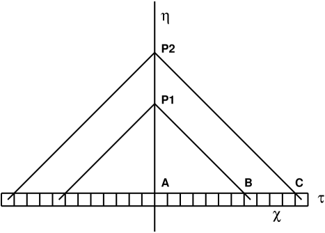
Figure 5: Buildup of $\langle{\mathbf{A}}^{2}\rangle_{\mathrm{nt}}$. Each box represents a spherical shell of radius $\chi$, thickness $\mathrm{d}\chi$, duration $\tau$. For clarity, only one time slice is shown; the plasma actually fills the whole volume from $\eta=0$ to the observation time.

The number density of particles in this shell, for a thermal distribution, is

$$\nu_{\mathrm{s}}=0.24T_{\mathrm{s}}^{3},$$ (58)

and the number of particles in the shell is then

$$\mathrm{d}N_{\mathrm{s}} = 4\pi(0.24T_{\mathrm{s}}^{3})R_{\mathrm{s}}^{3}\sinh^{2}\chi\,\mathrm{d}\chi$$ (59)

$$\equiv 4\pi(0.24)A_{\mathrm{M}}^{3/4}\sinh^{2}\chi\,\mathrm{d}\chi.$$

Here we have introduced, following Mannheim mann6 , the quantity $A_{\mathrm{M}}=R^{4}T^{4}$, which (at our current level of calculation) will be constant during the expansion, and therefore does not need another subscript, ‘s’ or ‘p’.

Multiplying (59) and (56) we get the contribution to $A_{2}^{2}$ from the particles in the shell. We convert this to $g^{\mu\nu}A_{\mu}A_{\nu}$ by multiplying by $g^{22}$:

$$4\pi(0.24)A_{\mathrm{M}}^{3/4}\sinh^{2}\chi\,\mathrm{d}\chi\left(2q\tau\right)^{2}$$

$$\times\langle V^{2}\rangle\langle\sin^{2}\theta\rangle\frac{\tanh^{2}(a\chi)}{R_{\mathrm{p}}^{2}\sinh^{2}\chi}.$$ (60)

The average of $\sin^{2}\theta$ over a sphere gives $2/3$. For the average of $V^{2}$ we reason as follows: if the effective $m^{2}$ of the particles were purely thermal, we could write $V^{2}=1/2$. But the effective mass actually increases with time as the ratio $p$ from (57) increases from zero towards one. So a better estimate of $V^{2}$ is $1/(2+p)$.

$\eta=0$ at the surface of the bubble, and $\eta=\eta_{\mathrm{p}}$ at the observation point. For some time slice at time $\eta$ between these two limits, we get the contribution of all spherical shells to $\langle{\mathbf{A}}^{2}\rangle_{\mathrm{nt}}$ by integrating from $\chi=0$ to the light cone at $\chi=\eta_{\mathrm{p}}-\eta$:

$$\frac{8\pi(0.24)}{3}A_{\mathrm{M}}^{3/4}\left(\frac{1}{2+p}\right)\left(2q\tau\right)^{2}\int_{0}^{\eta_{\mathrm{p}}-\eta}\!\!\mathrm{d}\chi\frac{\tanh^{2}(a\chi)}{R_{\mathrm{p}}^{2}}.\quad$$ (61)

We now have to sum over all time slices of duration $\tau$. The sum can be converted to an integral by multiplying by $\mathrm{d}\eta/\tau$:

$$\frac{32\pi(0.24)}{3}A_{\mathrm{M}}^{3/4}q^{2}\int_{0}^{\eta_{\mathrm{p}}}\!\!\mathrm{d}\eta\left(\frac{1}{2+p}\right)\tau$$

$$\times\int_{0}^{\eta_{\mathrm{p}}-\eta}\!\!\mathrm{d}\chi\frac{\tanh^{2}(a\chi)}{R_{\mathrm{p}}^{2}}.$$ (62)

In section IV we defined $\tau=\tau_{t}/R_{\mathrm{s}}(t)$. For $\tau_{t}$ we will simply use equation (3.24) from mont2 . The factor $U^{3}$ in the numerator will be of order $(2+p)^{-3/2}$; the quantity in the bracket in the denominator is of order unity and will be omitted. We then have, in our notation, $\tau_{t}=m^{2}(2+p)^{-3/2}/(8\pi\nu_{\mathrm{s}}q^{4}\ln\Lambda)$. For $m^{2}$ we will use the effective mass at time $t$. The purely thermal value is $q^{2}T_{\mathrm{s}}^{2}$, but we should multiply this by $(1+p)$ to include the non-thermal part also. We have $\nu_{\mathrm{s}}=0.24T_{\mathrm{s}}^{3}$, so

$$\tau = \frac{1+p}{8\pi\ln\Lambda(0.24)T_{\mathrm{s}}q^{2}R_{\mathrm{s}}(2+p)^{3/2}}$$ (63)

$$= \frac{1+p}{8\pi\ln\Lambda(0.24)q^{2}A_{\mathrm{M}}^{1/4}(2+p)^{3/2}}.$$

We can now get an expression for $p$ by using (63) in (62) and dividing by $T_{\mathrm{p}}^{2}$:

$$p = \frac{4}{3\ln\Lambda}A_{\mathrm{M}}^{3/4}q^{2}\int_{0}^{\eta_{\mathrm{p}}}\!\!\mathrm{d}\eta\left(\frac{1+p}{q^{2}A_{\mathrm{M}}^{1/4}(2+p)^{5/2}}\right)$$ (64)

$$\times\int_{0}^{\eta_{\mathrm{p}}-\eta}\!\!\mathrm{d}\chi\frac{\tanh^{2}(a\chi)}{R_{\mathrm{p}}^{2}T_{\mathrm{p}}^{2}}$$

$$= \frac{4}{3\ln\Lambda}\int_{0}^{\eta_{\mathrm{p}}}\!\!\mathrm{d}\eta\frac{1+p}{(2+p)^{5/2}}\int_{0}^{\eta_{\mathrm{p}}-\eta}\!\!\mathrm{d}\chi\tanh^{2}(a\chi)$$

$$= \frac{4}{3\ln\Lambda}\int_{0}^{\eta_{\mathrm{p}}}\!\!\mathrm{d}\eta\frac{1+p}{(2+p)^{5/2}}$$

$$\times\left\{\eta_{p}-\eta-\tanh[a(\eta_{p}-\eta)]/a\right\}.$$

This integral equation is surely not correct in detail, but it does provide a general picture of the buildup of $p$ from $p=0$ at $\eta_{p}=0$. We seek $\eta_{\mathrm{cw}}$, the value of $\eta_{p}$ for which $p=1$. Use $a=0.735$, as before, and for definiteness set $\ln\Lambda=10$; numerical solution then gives $\eta_{\mathrm{cw}}\approx 11$.

A remarkable feature of (64) is that not only has $A_{\mathrm{M}}$ disappeared, but also the coupling constant, $q$. The long-range character of the Coulomb interaction, however, is still apparent in $\ln\Lambda$. An equation of this sort might reasonably have been expected to yield a value of $\eta_{\mathrm{cw}}$ that was either extremely small, so the CW transition takes place almost immediately after the formation of the bubble, or extremely large, so the transition never takes place at all. Instead we get a value of $\eta_{\mathrm{cw}}$ that is within one or two orders of magnitude of unity.

As an example of the application of this result, we estimate, in appendix B, parameters in the model developed by Mannheim mann6 for conformal gravity.

One might think that in setting up potentials by the “classical prescription” of subsection VIII.4 we would find that at any point a large value of $\langle\mathbf{A}\rangle$ would develop, as well as $\langle{\mathbf{A}}^{2}\rangle_{\mathrm{nt}}$. But this is not so, once we treat the Universe as a quantum mechanical system. We must avoid being too specific about the state of distant matter, which we cannot investigate directly. We should not assume it is in a pure state; rather, it is a mixture, and all states compatible with the conservation laws will be present in the density matrix. In many situations, as emphasized by ter Haar terhaar , it is a matter of taste whether we adopt the statistical (ensemble) or quantum mechanical interpretation of the density matrix. In the language of Bell bell1 , “or” and “and” are equally acceptable. But this is not the case here; the quantum mechanical interpretation is the appropriate one. In an ordinary plasma in Minkowski space, only the particles within the Debye sphere will contribute to ${\mathbf{A}}$, and we do not have to concern ourselves with mixtures. But propagation in a curved space obliges us to consider very large numbers of particles at cosmological distances, and the introduction of a mixture is inevitable.

Like the distant Universe itself, $\langle{\mathbf{A}}^{2}\rangle$ will be a mixture, and the only meaningful quantities are averages. By symmetry, $\langle{\mathbf{A}}\rangle$ will be zero, but $\langle{\mathbf{A}}^{2}\rangle$ will not, so $q^{2}\langle{\mathbf{A}}^{2}\rangle$ can play the role of $m^{2}$.

XI INTRODUCTION OF CONDUCTIVITY

Up to this point we have been mainly concerned with potentials in the tail. But we have now to look more closely at the electric and magnetic fields in the main pulse for dipole propagation. These combine to give a Poynting vector directed outwards. In flat space, this vector falls off like $1/\chi^{4}$, which tends to zero even when integrated over the whole sphere. When we go to curved space, however, the Poynting vector tends to $(qV\sin\theta/\sinh\chi)^{2}$. The surface area of a sphere is $4\pi R^{2}\sinh^{2}\chi$, so the integral of the Poynting vector tends to a constant non-zero value. One effect of curvature is to continuously increase the energy of the plasma.

It seems unlikely this extra energy will remain in the form of pulses like those of figure 2. We know such pulses propagate unchanged in a flat space, but when they have traveled cosmological distances, so the curvature becomes noticeable, we should expect a gradual thermalization. We will model this thermalization by including a small, constant conductivity, $\sigma$, in our equations. Note that $\sigma$ is not directly related to the normal conductivity of the plasma, which (in our cosmological units) would be very high. $\sigma$ is just a device to represent the slow thermalization, and will have a value of order unity. For technical reasons, which we explain below, we choose $\sigma=1/(2\pi)$.

There are two reasons why we have to investigate the effect of $\sigma$:

1. The thermalization of the pulses raises the temperature of the plasma, and so tends to reduce the value of the ratio $p$.

2. The slow decline in the height of the pulses will probably reduce the value of $A$ in the tail, and this will also reduce the value of $p$.

The gradual transfer of energy to the plasma implies that the product $R(\eta)T(\eta)$ will not remain constant, as in a simple expansion, but will slowly increase. In this respect $\sigma$ simulates inflation, but on a much longer time scale.

XII Inclusion of conductivity: fields

The wave number, $k$, the permittivity, $\epsilon(n)$, and the conductivity, $\sigma$, satisfy the dispersion relation

$$k^{2}=n^{2}\epsilon(n)=n(n+4\pi i\sigma).$$ (65)

By analogy with Maxwell’s equations in flat space, the equations (17), (18) and (19) for our dipole fields become:

$$in\epsilon\sinh^{2}\chi f_{1}-2f_{3} = 0,$$ (66)

$$in\epsilon f_{2}-f_{3}^{\,\prime} = 0,$$ (67)

$$f_{1}-f_{2}^{\,\prime}+inf_{3} = 0.$$ (68)

XII.1 Magnetic field

From these we obtain an equation for $f_{3}$ alone:

$$\frac{d^{2}f_{3}}{d\chi^{2}}+\left(n^{2}\epsilon-\frac{2}{\sinh^{2}\chi}\right)f_{3}=0.$$ (69)

Writing $k^{2}$ for $n^{2}\epsilon$ this equation takes a familiar form; $f_{3}$ can be derived from the empty-space formula simply by writing $k$ for $n$ everywhere, except, of course, for the normalization function, which we denote now by $C_{3}(n,\sigma)$:

$$f_{3} = \frac{C_{3}(n,\sigma)\exp(ik\chi)}{2u}\left(1-2iku+u^{2}\right).$$ (70)

$C_{3}(n,\sigma)$ is most easily determined in flat space; this is sufficient since we only have to consider small distances. The calculation is done in Appendix C; see (129).

XII.2 Electric fields

(66) and (70) give the radial component of the electric field:

$$f_{1} = \frac{-iC_{3}(n,\sigma)\exp(ik\chi)(1-u^{2})^{2}}{4(n+4\pi i\sigma)u^{3}}$$ (71)

$$\times\left(1-2iku+u^{2}\right).$$

(67) and (70) give the transverse component of the electric field:

$$f_{2} = \frac{iC_{3}(n,\sigma)\exp(ik\chi)}{4(n+4\pi i\sigma)u^{2}}$$ (72)

$$\times\left[(1-u^{2})^{2}-2iku(1+u^{2})-4k^{2}u^{2}\right].$$

XII.3 Propagation of the magnetic field

The Fourier transform of the magnetic field becomes

$$F_{12} = \frac{-3qV(n+4\pi i\sigma)N_{1}(\theta)\sin(n\tau)\exp(ik\chi-in\eta)}{(3n+8\pi i\sigma)nu}$$ (73)

$$\times\left(1-2iku+u^{2}\right).$$

We can integrate around the pole at $n=0$ in the same way as before, except that we have to respect the branch points of $k$, at $n=0$ and $n=-4\pi i\sigma$. We have also to take account of the pole at $n=-8\pi i\sigma/3$. A suitable contour is shown in figure 6.

The integrals are straightforward, and the resulting propagation of $F_{12}$ is shown in figure 7. Notice that the pulses now show a tail that represents a reflected wave. This is unlikely to be significant in practice, because any irregularities in the plasma will tend to disrupt the coherence of the wave as it converges on the origin.

We note here for future reference that when $\eta\gg 1$ we can derive a simple asymptotic form for $F_{12}$ and $F_{20}$, using the fact that in the integration around the contour the integrand is concentrated near $n=0$. We just give the result:

$$F_{12} \approx 3qV\sin\theta\sqrt{\frac{\sigma}{\eta+\tau}}\exp\left(\frac{-\pi\sigma\chi^{2}}{\eta+\tau}\right),$$ (74)

$$F_{20} \approx F_{12}/(4\pi\sigma).$$ (75)

Figure 6: Contour for computing the magnetic field, $F_{12}$, when conductivity is included. The points on the negative imaginary axis labeled $A$ and $B$ are at $n=-8\pi i\sigma/3$ and $n=-4\pi i\sigma$, respectively. The contour is traversed in a clockwise sense.

Figure 7: Propagation of the magnetic field, $F_{12}$, in the presence of conductivity, $\sigma=1/2\pi$.

XIII Inclusion of conductivity: potentials

Here we follow the prescription of Landau and Lifshitz landau : use the same equations relating potentials and fields as in empty space, i.e. (39), (40) and (41), but modify the Lorenz condition by including the permittivity in the $h_{0}$ term:

$$in\epsilon\sinh^{2}\chi h_{0}+\frac{d}{d\chi}\left[\sinh^{2}\chi h_{1}\right]-2h_{2}=0.$$ (76)

XIII.1 Scalar potential

From these equations, as before, we can derive an equation for $h_{0}$ alone:

$$\frac{d^{2}h_{0}}{d\chi^{2}}+2\coth\chi\frac{dh_{0}}{d\chi}+\left(n^{2}\epsilon-\frac{2}{\sinh^{2}\chi}\right)h_{0}=0.$$ (77)

This is the same equation as we obtained for empty space, except that, just as for the magnetic field, in place of $n^{2}$ we must write $k^{2}\equiv n^{2}\epsilon$. (49) applies as before, provided we write $\alpha=\sqrt{k^{2}-1}$, and use a normalization function $C_{4}(n,\sigma)$ in place of $C_{2}(n)$.

This normalization function can be found from (40) and (71), in the limit $\chi\rightarrow 0$. We get, in place of (50),

$$C_{4}(n,\sigma)=\frac{iC_{3}(n,\sigma)}{4(n+4\pi i\sigma)}.$$ (78)

For the Fourier synthesis we need, in general, to use a more complicated contour than the one shown in figure 6, because we have to take account of the branch points of both $k$ and $\alpha$. With our choice of $\sigma=1/2\pi$, however, the branch points of $\alpha$ coalesce into a single point at $n=-i$, and the contour of figure 6 is adequate.

XIII.2 Vector potential

(52) holds, as in the case of zero conductivity. The first term on the right side of (52) comes from (72):

$$\frac{-if_{2}}{n} = \frac{C_{3}(n,\sigma)\exp(ik\chi)}{4n(n+4\pi i\sigma)u^{2}}$$ (79)

$$\times\left[(1-u^{2})^{2}-2iku(1+u^{2})-4k^{2}u^{2}\right].\quad$$

The second term on the right side of (52) comes from (49):

$$\frac{ih_{0}}{n} = \frac{iC_{4}(n,\sigma)\exp(i\alpha\chi)(1-u^{2})}{nu^{2}}$$ (80)

$$\times\left(1-2i\alpha u+u^{2}\right).$$

The two normalization functions are related by (78), and we also know $k^{2}=n(n+4\pi i\sigma)$. Combining, we get:

$$h_{2} = \frac{C_{3}(n,\sigma)}{4n(n+4\pi i\sigma)u^{2}}\left({\cal K_{\mathrm{\sigma}}}+{\cal A_{\mathrm{\sigma}}}\right),$$ (81)

$${\cal K_{\mathrm{\sigma}}} = e^{ik\chi}\left[(1-u^{2})^{2}-2iku(1+u^{2})-4k^{2}u^{2}\right],\quad$$ (82)

$${\cal A_{\mathrm{\sigma}}} = e^{i\alpha\chi}(1-u^{2})\left(-1+2i\alpha u-u^{2}\right).$$ (83)

XIII.3 Propagation of the vector potential

Combining (81) with (37), (129) and (10), and setting $-8\pi i\sigma/3=n_{p}$, we get

$$A_{2}=\frac{-qVN_{1}(\theta)\sin(n\tau)e^{-in\eta}}{2(n-n_{p})n^{2}u^{2}}\left({\cal K_{\mathrm{\sigma}}}+{\cal A_{\mathrm{\sigma}}}\right).$$ (84)

We note that going from (53) to (84) takes three simple steps:

1. Rename ${\cal N}$ and ${\cal A}$; call them ${\cal K}_{\sigma}$ and ${\cal A}_{\sigma}$, respectively.

2. In the final parenthesis, substitute $k$ for $n$ in both ${\cal K}_{\sigma}$ and ${\cal A_{\sigma}}$; this includes redefining $\alpha$ to be $\sqrt{k^{2}-1}$ rather than $\sqrt{n^{2}-1}$.

3. In the prefactor, change $n^{3}$ in the denominator to $n^{2}(n-n_{p})$.

(84) becomes (53) in the limit $\sigma\rightarrow 0$, as it should.

We transform to $\eta$, $\chi$, $\theta$, $\phi$ coordinates as before, by dividing (84) by $2\pi$ and integrating clockwise around the contour of figure 6. The result is shown in figure 8.

Figure 8: Propagation of the vector potential, $A_{2}$, in the presence of conductivity, $\sigma=1/2\pi$.

XIII.4 Asymptotic form of the vector potential

We can show easily that in the limit $\eta\rightarrow\infty$, $A_{2}$ satisfies a diffusion equation. The main terms come from the integral down the cut, and in this limit the integrand is concentrated close to $n=0$. This makes it possible, as for the fields, to obtain a simple expression for the asymptotic form:

$$A_{2} \approx \frac{3qV\tau\sin\theta}{16\pi}F(\sigma,\chi,\eta),$$ (85)

$$F(\sigma,\chi,\eta) = \left\{\frac{(1-u^{2})^{2}}{\sigma u^{2}}{\mathrm{erf}}\left(\chi\sqrt{\frac{\pi\sigma}{\eta}}\right)-\frac{4}{\sigma^{1/2}\eta^{3/2}u}\right.$$ (86)

$$\left.{}\times\left[(1+u^{2})\eta+4\pi\sigma u\chi\right]\exp\left(\frac{-\pi\sigma\chi^{2}}{\eta}\right)\right\}.\,$$

When $\chi$ is also large, of order $\sqrt{\eta}$, the term involving the error function is negligible compared to the others.

In figure 9 we plot $\sqrt{\eta}A_{2}$ against $\xi=\chi/\sqrt{\eta}$, with $A_{2}$ computed using the asymptotic formula. We see $\sqrt{\eta}A_{2}$ tending to a constant form; with our choice of abscissa, this is a Gaussian for large $\chi$ and $\eta$. For $\eta\geq 4$, this graph is indistinguishable from the one using integration around the contour.

Figure 9: $\sqrt{\eta}A_{2}$ plotted against $\xi=\chi/\sqrt{\eta}$, to demonstrate the asymptotic form. In this graph we use the asymptotic form (85) for the tail.

XIV The energy-transfer equation

We will now investigate the effect of a non-zero conductivity on the temperature of the plasma. We start from Weinberg wein2 , equation (4.7.9):

$$T^{\mu\nu}_{\;\;\;;\mu}=\frac{1}{\sqrt{g}}\frac{\partial}{\partial x^{\mu}}\left(\sqrt{g}T^{\mu\nu}\right)+\Gamma^{\nu}_{\mu\lambda}T^{\mu\lambda}.$$ (87)

This expression is zero for any value of $\nu$, but the most important one for us is $\nu=0$. We treat the plasma as a perfect fluid at rest in FRW coordinates $\eta$, $\chi$, $\theta$, $\phi$, so that the 4-velocity $\left(U^{0},U^{i}\right)$ has $U^{i}=0$, $i=1,2,3$. Since $g_{\mu\nu}U^{\mu}U^{\nu}=-1$ and $g_{00}=R^{2}(\eta)$, $U^{0}=1/R$.

Multiply (87) by $\sqrt{g}\,\mathrm{d}^{4}x\,U_{\nu}$, sum over $\nu$, and set the resulting expression equal to zero; we get

$$\sqrt{g}\,\mathrm{d}^{4}x\,U_{0}T^{\mu 0}_{\;\;\;;\mu}=0.$$ (88)

The left-hand side of this equation is a coordinate scalar with $\sqrt{g}\mathrm{d}^{4}x$ an element of proper volume. Expanding (88):

$$\sqrt{g}\,\mathrm{d}^{4}x\,U_{0}\left[\frac{1}{\sqrt{g}}\frac{\partial}{\partial x^{0}}\left(\sqrt{g}\,T^{00}\right)+\frac{1}{\sqrt{g}}\frac{\partial}{\partial x^{i}}\left(\sqrt{g}\,T^{i0}\right)\right.$$

$$\left.{}+\Gamma^{0}_{ij}T^{ij}+\Gamma^{0}_{00}T^{00}\right]=0.$$ (89)

From this we can derive an integrodifferential equation for $T^{00}$. Details are given in appendix D. The resulting equation is most simply written in terms of $A_{\mathrm{M}}(\eta)=R^{4}(\eta)T^{4}(\eta)\,\mathrm{(eV)^{4}\cdot m^{4}}$. A similar quantity was introduced in section X, but there it could be treated simply as a constant. Here we calculate its variation with time:

$$\dot{A}_{M}(\eta)-P_{4}\int_{0}^{\eta}\mathrm{d}\eta^{\,\prime}A_{M}^{3/4}(\eta^{\,\prime})\frac{\sigma(\eta-\eta^{\,\prime})}{2+p(\eta)}$$

$$\times\exp\left[-2\pi\sigma(\eta-\eta^{\,\prime})\right]=0,$$ (90)

$$P_{4}=3.97\times 10^{-7}\,\mathrm{eV\cdot m}.$$ (91)

Note that because of the appearance of the function $p(\eta)$, this equation by itself is not sufficient to calculate $A_{\mathrm{M}}$. We obtain an independent equation connecting these two functions in the next section.

XV MASS GENERATION: SECOND CALCULATION

We will now obtain an equation for the ratio $p(\eta)$ analogous to (64), but based on the asymptotic form (85) for the tail of the vector potential. In our previous calculation, where the tail of $A_{2}$ reached a constant asymptotic value, we could be sure that $p$ would rise monotonically; the only question was whether there would be factors of $A_{\mathrm{M}}$ that would make the increase far too fast or far too slow. (This is just what happens, for example, if we use quadrupole rather than dipole potentials.) In this second calculation, we can anticipate that there will not be any unwanted factors of $A_{\mathrm{M}}$, but only a detailed calculation will show whether $p$ continues to rise with $\eta$.

The analog of (59) is

$$\mathrm{d}N_{\mathrm{s}}=4\pi(0.24)A_{\mathrm{M}}^{3/4}(\eta_{\mathrm{s}})\sinh^{2}\chi\,\mathrm{d}\chi.$$ (92)

To get the contribution to $A_{2}^{2}$ at $\eta_{\mathrm{p}}$ from the particles in the shell, we multiply (92) by $A_{2}^{2}[\sigma,\chi,(\eta_{\mathrm{p}}-\eta_{\mathrm{s}})]$, with $A_{2}(\sigma,\chi,\eta)$ given by (85).

Proceeding as before we get the analog of (62):

$$\frac{2\pi(0.24)q^{2}}{3R^{2}(\eta_{\mathrm{p}})}\int_{0}^{\eta_{\mathrm{p}}}\mathrm{d}\eta_{\mathrm{s}}\left(\frac{A_{\mathrm{M}}^{3/4}(\eta_{\mathrm{s}})}{2+p(\eta_{\mathrm{s}})}\right)\tau$$

$$\times\int_{0}^{\eta_{\mathrm{p}}-\eta_{\mathrm{s}}}\!\!\mathrm{d}\chi F^{2}\left[\sigma,\chi,(\eta_{\mathrm{p}}-\eta_{\mathrm{s}})\right],$$ (93)

with $F_{0}$ given by (86).

The collision time, $\tau$, will be given by

$$\tau=\frac{(1+p)}{8\pi\ln\Lambda(0.24)q^{2}A_{\mathrm{M}}^{1/4}(\eta_{\mathrm{s}})(2+p)^{3/2}}.$$ (94)

We can now get an expression for $p$ by using (94) in (93) and dividing by $T^{2}(\eta_{\mathrm{p}})$:

$$p(\eta_{\mathrm{p}}) = \frac{3}{256\pi^{2}\ln\Lambda A_{\mathrm{M}}^{1/2}(\eta_{\mathrm{p}})}$$ (95)

$$\times\int_{0}^{\eta_{\mathrm{p}}}\!\!\mathrm{d}\eta_{\mathrm{s}}\left(\frac{\left[1+p(\eta_{\mathrm{s}})\right]A_{\mathrm{M}}^{1/2}(\eta_{\mathrm{s}})}{\left[2+p(\eta_{\mathrm{s}})\right]^{5/2}}\right)$$

$$\times\int_{0}^{\eta_{\mathrm{p}}-\eta_{\mathrm{s}}}\!\!\mathrm{d}\chi F^{2}\left[\sigma,\chi,(\eta_{\mathrm{p}}-\eta_{\mathrm{s}})\right],$$

with $F_{0}$ given by (86).

XV.1 Calculation of $\bm{p}$ and $\bm{A_{\mathrm{M}}}$

As before, we set $\ln\Lambda=10$ for definiteness. Simultaneous numerical solution of (90) and (95) is straightforward, but we need to choose a starting value for $A_{\mathrm{M}}$. We have used two extreme values:

1. $A_{\mathrm{M}}$ starts at $2.5\times 10^{-26}\,\mathrm{eV^{4}\cdot m^{4}}$. This is a “natural” value, in the sense that the Universe begins with the typical wavelength of the radiation approximately equal to the radius, $R$. $p$ becomes equal to unity around $\eta_{\mathrm{cw}}=1650$.

2. $A_{\mathrm{M}}$ starts at $2.5\times 10^{74}\,\mathrm{eV^{4}\cdot m^{4}}$. This is approximately equal to the observed value today. $p$ becomes equal to unity around $\eta_{\mathrm{cw}}=480$.

These values of $\eta_{\mathrm{cw}}$ are significantly larger than the previous value of $11$ when $\sigma=0$, but they are still within a few orders of magnitude of unity. The most important feature of this calculation is that it shows $p(\eta)$ does continue to rise, even when $\sigma\neq 0$, so a CW transition will still eventually become possible.

XVI CONCLUSION

We have considered the problem of the generation of a particle mass scale in a theory in which this scale is not determined by the gravitational constant, through $m_{\mathrm{planck}}$. Conformal gravity mann6 may turn out to be a theory of this type. We find that in such a theory distant matter is significant in an unexpected way, and the mass scale is to a large extent classically determined. Since the mass scale develops through the agency of the classical vector potential, it is bound to appear in any model universe containing charged particles, providing the underlying space has sufficient curvature and allows enough time.

Many questions remain, among them the following:

1. Will a CW transition necessarily take place as the ratio $\langle{\mathbf{A}}^{2}\rangle_{\mathrm{nt}}/\langle{\mathbf{A}}^{2}\rangle_{\mathrm{th}}$ approaches unity?

2. Is the tail of ${\mathbf{A}}$ important only in the early Universe, or are there other places, regions of high gravitational fields, where its effects can be observed even now?

3. How does the real complicated early plasma determine such things as the collision time?

4. Finally, perhaps most important, can we really expect ${\mathbf{A}}$ to propagate over cosmological distances? We have taken findings from ordinary plasma theory and used them in the very different circumstances of the early Universe.

These considerations are beyond the scope of this paper, which is solely concerned with the interplay, in a simple model, of quantum mechanics (density matrix, the Lagrangian for a scalar field, the Coleman-Weinberg transition) and the classical equations of propagation of the ordinary vector potential in a FRW space of negative curvature.

Appendix A HYPERGEOMETRIC FUNCTIONS

Hypergeometric functions are usually difficult to handle because they depend on three parameters. For all the hypergeometric functions we need in this paper, however, the parameters $a$, $b$, and $c$ can be expressed in terms of two numbers, an integer, $d$, and a quantity $\alpha$ which is complex in general:

$$a=d+i\alpha;\,\,\,b=d-i\alpha;\,\,\,c=d+1/2.$$ (96)

Hypergeometric functions that satisfy this condition can be expressed in terms of elementary functions. For proof we use formulae from Abramowitz and Stegun (absteg , hereafter AS). Define $\mu=(1-\cosh(\chi))/2$. Then, for $d=0$, AS (15.1.17) gives, in our notation, $F(i\alpha,-i\alpha;1/2;\mu)=F[i\alpha,-i\alpha;1/2;\sin^{2}(i\chi/2)]=\cos(\alpha\chi)$. Other functions can be obtained by successive differentiation or integration using AS (15.2.1). If $\alpha$ happens to be purely real or purely imaginary the hypergeometric functions are real.

For dipole propagation the only functions we need are those with $d=-1$ and $d=2$. They are listed below, together with the functions with intermediate values of $d$. We can replace the argument $\mu$ by $\chi$:

$$F(-1+i\alpha,-1-i\alpha;-1/2;\chi) =$$ (97)

$$\cosh\chi\cos(\alpha\chi)+\alpha\sinh\chi\sin(\alpha\chi),$$

$$F(i\alpha,-i\alpha;1/2;\chi) = \cos(\alpha\chi),$$ (98)

$$F(1+i\alpha,1-i\alpha;3/2;\chi) = \frac{\sin(\alpha\chi)}{\alpha\sinh\chi},$$ (99)

$$F(2+i\alpha,2-i\alpha;5/2;\chi) =$$ (100)

$$\frac{-3[\alpha\sinh\chi\cos(\alpha\chi)-\cosh\chi\sin(\alpha\chi)]}{\alpha(1+\alpha^{2})\sinh^{3}\chi}.$$

Appendix B Parameters in the model of Mannheim

Mannheim finds that the field equations of conformal gravity take on a particularly simple form in the context of a FRW space, as in cosmological investigations. He obtains (mann6 , equation (230)) the following expression for the expansion factor, $R$, as a function of the ordinary time, $t$, assuming the matter in the Universe is in the form of radiation and the space has negative curvature ($k=-1$):

$$R^{2}(t)=\frac{(\beta_{\mathrm{M}}-1)}{2\alpha_{\mathrm{M}}}+\frac{\beta_{\mathrm{M}}\sinh^{2}(\alpha_{\mathrm{M}}^{1/2}ct)}{\alpha_{\mathrm{M}}}.$$ (101)

$\alpha_{\mathrm{M}}$ and $\beta_{\mathrm{M}}$ are real, positive parameters. $\beta_{\mathrm{M}}$ is dimensionless and greater than unity; $\alpha_{\mathrm{M}}$ has dimension ${\mathrm{length}}^{-2}$. (We write $\alpha_{\mathrm{M}}$ rather than Mannheim’s $\alpha$ to prevent any possible confusion if $\alpha$ is used elsewhere, for example to denote the fine structure constant; we use the same convention for other parameters in Mannheim’s model.) We will use (101) for the whole range of time from $t=0$ to the present, recognizing that this will be inaccurate during the mass-dominated phase of the expansion. We estimate this time interval below.

Time $t=0$ corresponds to the surface of the bubble. Here $R$ has a non-zero minimum value, $R_{\mathrm{min}}=[(\beta_{\mathrm{M}}-1)/(2\alpha_{\mathrm{M}})]^{1/2}$, and a maximum temperature, $T_{\mathrm{max}}$. Mannheim defines a third parameter, $A_{\mathrm{M}}$, by

$$A_{\mathrm{M}}=R^{4}(t)T^{4}(t).$$ (102)

We will not try to explain the large size of $A_{\mathrm{M}}$, but will make essential use of the fact that (in this simple model, at least) it has a constant value during the expansion. If we can determine the three parameters $\alpha_{\mathrm{M}}$, $\beta_{\mathrm{M}}$ and $A_{\mathrm{M}}$ we can derive the values of all the rest of Mannheim’s parameters for this model.

Equation (101) leads to an expression for the acceleration parameter, $q_{0}$. By comparing this with the value obtained from supernova observations, Mannheim finds that $\alpha_{\mathrm{M}}^{1/2}ct\approx 0.7$ at the present time, so that $\alpha_{\mathrm{M}}^{1/2}$ is of the order of the inverse Hubble distance. $A_{\mathrm{M}}$ can be estimated from the current CMB spectrum and the Hubble distance; we will use a value of $A_{\mathrm{M}}^{1/4}=1.68\times 10^{29}$.

The parameter $\beta_{\mathrm{M}}$ is harder to estimate. The temperature evolution of the Universe is given by the following equation (mann6 , equation (232)):

$$\frac{T_{\mathrm{max}}^{2}}{T^{2}}=1+\frac{2\beta_{\mathrm{M}}\sinh^{2}(\alpha_{\mathrm{M}}^{1/2}ct)}{(\beta_{\mathrm{M}}-1)}.$$ (103)

Since $T_{\mathrm{max}}\gg T_{0}$, where $T_{0}$ is the current temperature, $\beta_{\mathrm{M}}$ must be extremely close to $1$. It is therefore convenient to define a new parameter, $\delta_{\mathrm{M}}=\beta_{\mathrm{M}}-1$, with $0<\delta_{\mathrm{M}}\ll 1$. Equation (101) then shows that $\delta_{\mathrm{M}}$ has an appreciable effect on $R(t)$ only at the very earliest times. We will estimate $\delta_{\mathrm{M}}$ below.

Mannheim suggests that the CW phase transition occurs at an intermediate temperature, $T_{\mathrm{V}}$, with $T_{\mathrm{V}}^{2}\approx T_{\mathrm{max}}T_{0}$. He regards the mechanism of this phase transition as a matter for particle physics, and does not consider it in detail. In our model the transition occurs at a considerably higher temperature, and appears not to be connected to $T_{\mathrm{V}}$.

Define $x=\alpha^{1/2}t$, with $x_{0}=\alpha^{1/2}t_{0}=0.7$ the current value. The current CMB temperature is $T_{0}=2.3\times 10^{-4}{\mathrm{eV}}$. The CW transition will occur at a temperature of about $T_{\mathrm{cw}}=10^{9}{\mathrm{eV}}$, so, since $\delta_{\mathrm{M}}\ll x_{\mathrm{cw}}\ll 1$:

$$x_{\mathrm{cw}} = \sinh(0.7)(2.3\times 10^{-4})/10^{9}$$ (104)

$$= 1.7\times 10^{-13},$$

$$\eta_{0}-\eta_{\mathrm{cw}} = \int_{x_{\mathrm{cw}}}^{x_{0}}\!\frac{\mathrm{d}x}{\sinh(x)}$$ (105)

$$= \ln\left(\frac{\tanh(x_{0}/2)}{\tanh(x_{\mathrm{cw}}/2)}\right)=29.$$

Also, since $x_{cw}\ll 1$,

$$\eta_{\mathrm{cw}} = \int_{0}^{x_{\mathrm{cw}}}\!\!\frac{\mathrm{d}x}{\left[\delta_{\mathrm{M}}/2+x^{2}\right]^{1/2}}$$ (106)

$$= \ln\left[\frac{x+\sqrt{\delta_{\mathrm{M}}/2+x^{2}}}{\sqrt{\delta_{\mathrm{M}}/2}}\right]$$

$$= \ln\left(2^{3/2}x_{\mathrm{cw}}\delta_{\mathrm{M}}^{-1/2}\right),$$

$$x_{\mathrm{cw}} = 2^{-3/2}\delta_{\mathrm{M}}^{1/2}\exp(\eta_{\mathrm{cw}}),$$ (107)

$$x_{\mathrm{min}} = 2^{-1/2}\delta_{\mathrm{M}}^{1/2},$$ (108)

$$T_{\mathrm{max}} = T_{\mathrm{cw}}x_{\mathrm{cw}}/x_{\mathrm{min}}$$ (109)

$$= 0.5\times 10^{9}\times\exp(\eta_{\mathrm{cw}})=3\times 10^{13}\,{\mathrm{eV}},$$

where we have used $\eta_{\mathrm{cw}}=11$, as derived from (64).

Equation (232) of mann6 gives

$$\delta_{\mathrm{M}} = 2(0.76)^{2}\left(\frac{2.3\times 10^{-4}}{3\times 10^{13}}\right)^{2}=6.8\times 10^{-35},\qquad$$ (110)

$$T_{\mathrm{V}} = T_{\mathrm{max}}(\delta_{\mathrm{M}}/2)^{1/4}=7\times 10^{4}\,{\mathrm{eV}}.$$ (111)

Our equation (101), Mannheim’s expression for $R^{2}(t)$, will become inaccurate during the mass-dominated phase of the expansion, between $T=T_{\mathrm{cw}}$ and $T_{\mathrm{V}}$. This corresponds to an interval of conformal time of about $10$, compared to $40$ for the whole interval from $t=0$ to the present.

Appendix C Normalization with conductivity

In this appendix we will work in the usual spherical polar coordinates, and make connection with Riemannian coordinates when necessary.

Suppose we have a dipole at the origin, oscillating with time dependence $\exp(-i\omega t)$ in the $z$ direction. The surrounding medium is of uniform conductivity, $\overline{\sigma}$, so that the current density, ${\mathbf{j}}$, is given by ${\mathbf{j}}=\overline{\sigma}{\mathbf{E}}$. We will analyze this system by imagining a small sphere of radius $r_{1}$ cut out of the medium surrounding the dipole. Induced currents flowing in the medium will cause surface charges to appear on the sphere, and the total dipole moment will be the sum of the original dipole moment and that due to the induced charges. We assume the permittivity and magnetic susceptibility are essentially unity, so ${\mathbf{D}}={\mathbf{E}}$ and ${\mathbf{B}}={\mathbf{H}}$. In such a system $\nabla\cdot{\mathbf{j}}=0$ follows from Maxwell’s equations, so there are no volume charges in the medium.

The dipole moment at the center of the small sphere is denoted by $D_{\mathrm{t}rue}=D(\omega)\exp(-i\omega t)$, where $D(\omega)$ is the true dipole strength at angular frequency $\omega$. The induced dipole moment due to the surface charges is $D_{\mathrm{i}nd}$, so the total dipole moment is $D_{\mathrm{t}ot}=D_{\mathrm{t}rue}+D_{\mathrm{i}nd}$.

Just outside the sphere the electrostatic potential is given by

$$\Phi=D_{\mathrm{t}ot}P_{1}(\cos\theta)/r_{1}^{2},$$ (112)

where $P_{1}(\cos\theta)=cos\theta$. The radial component of ${\mathbf{E}}$ is given by

$$E_{r}=2D_{\mathrm{t}ot}P_{1}(\cos\theta)/r_{1}^{3}.$$ (113)

The surface charge density, $s$, obeys the relation

$$\frac{ds}{dt}=-j_{r}\;,$$ (114)

where $j_{r}$ is evaluated just outside the sphere. This gives

$$s=\frac{-i\overline{\sigma}E_{r}}{\omega}=s_{0}P_{1}(\cos\theta),$$ (115)

where

$$s_{0}=\frac{-2i\overline{\sigma}D_{\mathrm{t}ot}}{r_{1}^{3}\omega}\;.$$ (116)

The induced dipole moment, $D_{\mathrm{i}nd}$, is then given by an integral over the surface of the sphere:

$$D_{\mathrm{i}nd} = 2\pi\int_{0}^{\pi}d\theta\sin\theta r_{1}^{2}[s_{0}P_{1}(\cos\theta)][r_{1}^{2}P_{1}(\cos\theta)]$$ (117)

$$= \left(\frac{-4\pi i\overline{\sigma}}{\omega}\right)\left(\frac{2}{3}\right)D_{\mathrm{t}ot}\,,$$

giving

$$D_{\mathrm{t}ot} = D_{\mathrm{t}rue}+D_{\mathrm{i}nd}$$ (118)

$$= \frac{3\omega D_{\mathrm{t}rue}}{3\omega+8\pi i\overline{\sigma}}\,.$$

We set $H_{\phi}=C_{5}(\omega,\overline{\sigma})N_{1}(\theta)h(r)\exp(-i\omega t)$, where $C_{5}(\omega,\overline{\sigma})$ is the normalizing function we are looking for, $N_{1}=dP_{1}/d\theta$, and $h(r)$ satisfies

$$\frac{d^{2}h}{dr^{2}}+\frac{2}{r}\frac{dh}{dr}-\frac{2h}{r^{2}}+\kappa^{2}h=0\;,$$ (119)

with $\kappa^{2}=\omega(\omega+4\pi i\overline{\sigma})$. We choose the solution that represents outgoing waves, so

$$h(r) = h_{1}^{(1)}(\kappa r)$$ (120)

$$= \left(-\frac{i}{(\kappa r)^{2}}-\frac{1}{\kappa r}\right)e^{i\kappa r}.$$

Here $h_{1}^{(1)}(\kappa r)$ is the spherical Bessel function defined in AS, ch. 10.

The Maxwell equation $\nabla\times{\mathbf{H}}=-i(\omega+4\pi i\overline{\sigma}){\mathbf{E}}$ then gives

$$E_{r}=\frac{-2iC_{5}(\omega,\overline{\sigma})P_{1}(\cos\theta)h_{1}^{(1)}(\kappa r)\exp(-i\omega t)}{r(\omega+4\pi i\overline{\sigma})}.$$ (121)

For small $r$ this becomes:

$$E_{r}=\frac{-2C_{5}(\omega,\overline{\sigma})P_{1}(\cos\theta)\exp(-i\omega t)}{\kappa^{2}r^{3}(\omega+4\pi i\overline{\sigma})}.$$ (122)

But also, for small $r$, we have (113), so

$$C_{5}(\omega,\overline{\sigma}) = \frac{-3\omega\kappa^{2}(\omega+4\pi i\overline{\sigma})D(\omega)}{(3\omega+8\pi i\overline{\sigma})},$$ (123)

$$H_{\phi} = \frac{-3\omega\kappa^{2}(\omega+4\pi i\overline{\sigma})D(\omega)}{(3\omega+8\pi i\overline{\sigma})}$$ (124)

$$\times N_{1}(\theta)h_{1}^{(1)}(\kappa r)\exp(-i\omega t),$$

$$E_{r} = \frac{6i\omega\kappa^{2}D(\omega)P_{1}(\theta)h_{1}^{(1)}(\kappa r)\exp(-i\omega t)}{r(3\omega+8\pi i\overline{\sigma})}.\qquad\quad$$ (125)

In this appendix we have used ordinary polar coordinates in flat space. We need now to transform to coordinates of a FRW flat space, with metric

$$\mathrm{d}s^{2} = R^{2}(\eta)\left(-\mathrm{d}\eta^{2}+\mathrm{d}\chi^{2}+\chi^{2}\,\mathrm{d}\theta^{2}\right.$$ (126)

$$\left.{}+\chi^{2}\sin^{2}\theta\,\mathrm{d}\phi^{2}\right),$$

To get from $H_{\phi}$ of (124) to $F_{12}$ of (13), in the flat FRW metric (126), we first follow Weinberg wein2 , ch. 4, sec. 8, and multiply by $\chi$. We then convert from $t$ to $\eta$ and $r$ to $\chi$ by multiplying by $R^{2}(\eta)$. We also convert $\omega$ to $n$, $\kappa$ to $k$ and $\overline{\sigma}$ to $\sigma=R(\eta)\overline{\sigma}$:

$$F_{12} = \frac{-3nk^{2}(n+4\pi i\sigma)D(n)}{R(\eta)(3n+8\pi i\sigma)}$$ (127)

$$\times N_{1}(\theta)\chi h_{1}^{(1)}(k\chi)\exp(-in\eta).$$

We can obtain the corresponding function in curved space by multiplying (70) by $N_{1}(\theta)\exp(-in\eta)$:

$$F_{12} = \frac{C_{3}(n,\sigma)N_{1}(\theta)\exp[i(k\chi-n\eta)]}{2u}$$ (128)

$$\times\left(1-2iku+u^{2}\right).$$

We can now find $C_{3}(n,\sigma)$ by matching (127) with (128) for small $\chi$:

$$C_{3}(n,\sigma)=\frac{3in(n+4\pi i\sigma)D(n)}{R(\eta)(3n+8\pi i\sigma)}.$$ (129)

With $D(n)$ given by (10), we can check that in the limit $\sigma\rightarrow 0$, (129) tends to (32), as it should.

Appendix D Derivation of the energy-transfer equation

In this appendix we present details of the derivation of the energy-transfer equation (90), starting from equation (89):

$$\sqrt{g}\,\mathrm{d}^{4}x\,U_{0}\left[\frac{1}{\sqrt{g}}\frac{\partial}{\partial x^{0}}\left(\sqrt{g}\,T^{00}\right)+\frac{1}{\sqrt{g}}\frac{\partial}{\partial x^{i}}\left(\sqrt{g}\,T^{i0}\right)\right.$$

$$\left.{}+\Gamma^{0}_{ii}T^{ii}+\Gamma^{0}_{00}T^{00}\right]=0.$$ (130)

Write this as

$$z_{1}+z_{2}+z_{3}+z_{4}=0,$$ (131)

where the $z_{i}$ are derived from the four terms in the bracket in (130). The strategy will be to get an expression for $z_{2}$ from the propagation of $\mathbf{E}$ and $\mathbf{H}$. We combine this with $z_{1}$, $z_{3}$ and $z_{4}$, and arrive at an integrodifferential equation for $T^{00}$.

D.1 Calculation of $\bm{z_{1}}$

We consider first the effect of a single source particle at the origin of coordinates, and let the duration of our 4-volume be $\Delta x^{0}$. Our coordinate volume $\mathrm{d}\chi\mathrm{d}\theta\mathrm{d}\phi$ is a small part of a spherical shell of radius $\chi$ surrounding the source particle. Then $z_{1}$ in (131) is given by

$$z_{1} = \Delta x^{0}U_{0}\frac{\partial}{\partial x^{0}}\left(\sqrt{g}\,T^{00}\right)\mathrm{d}\chi\mathrm{d}\theta\mathrm{d}\phi$$ (132)

$$= R^{4}\left(4\dot{R}T^{00}+R\dot{T}^{00}\right)\sinh^{2}\chi\sin\theta\Delta\eta\mathrm{d}\chi\mathrm{d}\theta\mathrm{d}\phi.\qquad$$

D.2 Calculation of $\bm{z_{2}}$

For $z_{2}$ in (131) the only relevant derivative is $\partial/\partial\chi$, and we get

$$z_{2} = \Delta x^{0}\mathrm{d}\theta\,\mathrm{d}\phi\,U_{0}\Delta\left(\sqrt{g}\,T^{10}\right)$$ (133)

$$= \Delta\eta R\frac{\partial}{\partial\chi}\left(\sqrt{g}T^{10}\right)\mathrm{d}\chi\mathrm{d}\theta\mathrm{d}\phi.$$

Here $\Delta(\sqrt{g}\,T^{10})$ is the net outward flux from the shell, for a pulse that protrudes on both sides. The pulse is, of course, attenuated on the outward side, so the total outward flux is negative.

D.3 Calculation of $\bm{z_{3}}$ and $\bm{z_{4}}$

To compute $z_{3}$ and $z_{4}$ in (131) we start from Weinberg (5.4.2):

$$T^{\mu\nu}=pg^{\mu\nu}+(p+\rho)U^{\mu}U^{\nu}.$$ (134)

The only Christoffel symbols we need are $\Gamma^{0}_{00}=\dot{R}/R$ and $\Gamma^{0}_{ij}=\dot{R}g_{ij}/R^{3}$, where a dot denotes $\partial/\partial\eta$, and $i,\,j$ take values 1, 2, 3. Then

$$T^{00} = \frac{-p}{R^{2}}+\frac{p+\rho}{R^{2}}=\frac{\rho}{R^{2}},$$ (135)

$$T^{ij} = pg^{ij},$$ (136)

$$\Gamma^{0}_{\mu\lambda}T^{\mu\lambda} = \frac{\dot{R}\rho}{R^{3}}+\frac{\dot{R}p\,g_{ij}\,g^{ij}}{R^{3}}$$ (137)

$$= \frac{2\rho\dot{R}}{R^{3}}\quad\mathrm{if}\quad p=\rho/3.$$

We now have

$$z_{3}+z_{4} = U_{0}\frac{2\rho\dot{R}}{R^{3}}\Delta x^{0}\mathrm{d}\chi\,\mathrm{d}\theta\,\mathrm{d}\phi\,\sqrt{g}$$ (138)

$$= 2T^{00}\dot{R}\Delta\eta\sqrt{g}\mathrm{d}\chi\mathrm{d}\theta\mathrm{d}\phi.$$

D.4 Energy-transfer equation in terms of $\bm{T^{\mu\nu}}$

Using (132), (133) and (138) in (131) we get

$$4\dot{R}T^{00}+R\dot{T}^{00}+\frac{R}{\sinh^{2}\chi}\frac{\partial}{\partial\chi}\left(T^{10}\sinh^{2}\chi\right)$$

$${}+2\dot{R}T^{00} = 0,$$

$$\frac{6\dot{R}T^{00}}{R}+\dot{T}^{00}+\frac{1}{\sinh^{2}\chi}\frac{\partial}{\partial\chi}\left(T^{10}\sinh^{2}\chi\right) = 0.\qquad$$ (139)

We must now develop this equation in two ways:

1. Express the first two terms as functions of the temperature, $T(\eta)$.

2. Sum over all the source charges that contribute to $T^{10}$. Since we are concerned here with the main pulse, not the tail, this implies an integration along the light cone.

D.5 Expression of $\bm{T^{00}}$ in terms of $\bm{T(\eta)}$

We will measure temperature in electron-volts, $R$ in meters, and will assume the energy density is given in terms of the temperature by the familiar formulae for electromagnetic radiation (we will clearly miss a numerical factor here when dealing with the real plasma, but the overall relationship will be correct). Denote by $q_{\mathrm{MKS}}$ the elementary charge in MKS units, and let the energy density be $\rho$. Then

$$\rho = P_{1}T^{4}\,\mathrm{J\cdot m^{-3}},$$

$$P_{1} = \frac{\pi^{2}}{15}q_{\mathrm{MKS}}^{4}\cdot\hbar^{-3}\cdot c^{-3}$$ (140)

$$= \frac{\pi^{2}\left(1.6\times 10^{-19}\right)^{4}}{15\left(1.05\times 10^{-34}\right)^{3}\left(3\times 10^{8}\right)^{3}}$$

$$= 13.8\,\mathrm{\left(eV\right)^{-4}\cdot J\cdot m^{-3}},$$ (141)

$$T^{00} = \frac{P_{1}T^{4}(\eta)}{R^{2}(\eta)}\,\mathrm{J\cdot m^{-5}},$$ (142)

$$\dot{T}^{00} = \frac{4P_{1}T^{3}(\eta)\dot{T}(\eta)}{R^{2}(\eta)}-\frac{2P_{1}T^{4}(\eta)\dot{R}(\eta)}{R^{3}(\eta)}\,\mathrm{J\cdot m^{-5}}.\qquad$$ (143)

D.6 Integrating along the light cone

Using the asymptotic forms (74) and (75) for the fields, we obtain

$$T^{10} = -g^{00}g^{11}g^{22}F_{12}F_{20}$$ (144)

$$= \frac{(3qV\sin\theta)^{2}}{R^{6}(\eta)\sinh^{2}\chi}\frac{1}{4\pi(\eta+\tau)}\exp\left(\frac{-2\pi\sigma\chi^{2}}{\eta+\tau}\right),\quad\quad\;$$

$$\frac{\partial}{\partial\chi}\left(T^{10}\sinh^{2}\chi\right) =$$ (145)

$$\frac{-(3qV\sin\theta)^{2}\sigma\chi}{R^{6}(\eta)(\eta+\tau)^{2}}\exp\left(\frac{-2\pi\sigma\chi^{2}}{\eta+\tau}\right).\quad$$

This form refers to a single source particle. To get the total $T^{10}$ term in (139) we must integrate along the light cone. We will need the number density, which we write as $P_{2}T^{3}$, with the constant $P_{2}$ defined as for electromagnetic radiation:

$$P_{2} = \frac{2}{\pi^{2}}\zeta(3)\frac{q_{\mathrm{MKS}}^{3}}{\hbar^{3}c^{3}}$$ (146)

$$= 0.24\left[\frac{1.6\times 10^{-19}}{\left(1.05\times 10^{-34}\right)\left(3\times 10^{8}\right)}\right]^{3}$$

$$= 3.15\times 10^{20}\,\mathrm{\left(eV\right)^{-3}\cdot m^{-3}}.$$

We can now use (145) to write an expression for the total $T^{10}$ term in (139). We neglect $\tau$ in comparison with $\eta$, and write $\eta-\eta^{\,\prime}$ in place of $\eta$. We also express the charge $q$, which is in Gaussian units, in terms of $q_{\mathrm{MKS}}$:

$$q=\frac{1}{\sqrt{4\pi\epsilon_{0}}}q_{\mathrm{MKS}}\,,$$ (147)

with $\epsilon_{0}=(1/36\pi)\times 10^{-9}\,\mathrm{C^{2}\cdot J^{-1}\cdot m^{-1}}$.

$$\left[\frac{1}{\sinh^{2}\chi}\frac{\partial}{\partial\chi}\left(T^{10}\sinh^{2}\chi\right)\right] = \frac{-1}{R^{6}(\eta)}\int_{0}^{\eta}\mathrm{d}\eta^{\,\prime}\int_{0}^{\infty}\mathrm{d}\chi\delta(\chi-\eta+\eta^{\,\prime})\left[P_{2}T^{3}(\eta^{\,\prime})\right]$$ (148)

$$\times\left(4\pi R^{3}(\eta^{\,\prime})\sinh^{2}\chi\right)\left(\frac{1}{\sinh^{2}\chi}\right)\frac{(3q_{\mathrm{MKS}})^{2}\langle V^{2}\rangle\langle\sin^{2}\theta\rangle\sigma\chi}{4\pi\epsilon_{0}(\eta-\eta^{\,\prime})^{2}}\exp\left(\frac{-2\pi\sigma\chi^{2}}{\eta-\eta^{\,\prime}}\right)\Delta\eta\,.\quad$$

As in section X we set $\langle V^{2}\rangle\approx 1/(2+p(\eta))$ and $\langle\sin^{2}\theta\rangle=2/3$; we also define a new constant $P_{3}$:

$$P_{3} = P_{2}\times 36\pi\times\left(2/3\right)\times\left(1.6\times 10^{-19}\right)^{2}\times\left(9\times 10^{9}\right)$$ (149)

$$= 5.47\times 10^{-6}\,\mathrm{\left(eV\right)^{-3}\cdot J\cdot m^{-2}},$$

$$\left[\frac{1}{\sinh^{2}\chi}\frac{\partial}{\partial\chi}\left(T^{10}\sinh^{2}\chi\right)\right] = \frac{-P_{3}}{R^{6}(\eta)}\int_{0}^{\eta}\mathrm{d}\eta^{\,\prime}\frac{T^{3}(\eta^{\,\prime})R^{3}(\eta^{\,\prime})}{2+p(\eta)}\sigma(\eta-\eta^{\,\prime})\exp\left[-2\pi\sigma(\eta-\eta^{\,\prime})\right]\Delta\eta\,.$$ (150)

D.7 Final form of the energy-transfer equation

Using (142), (143) and (150) in (139):

$$4P_{1}T^{3}(\eta)\dot{T}(\eta)R^{4}(\eta)+4P_{1}T^{4}(\eta)R^{3}(\eta)\dot{R}(\eta)$$

$${}-P_{3}\int_{0}^{\eta}\mathrm{d}\eta^{\,\prime}\frac{T^{3}(\eta^{\,\prime})R^{3}(\eta^{\,\prime})}{2+p(\eta)}\sigma(\eta-\eta^{\,\prime})$$

$$\times\exp\left[-2\pi\sigma(\eta-\eta^{\,\prime})\right]=0.$$ (151)

This equation can be written in terms of the single variable $A_{\mathrm{M}}(\eta)\equiv T^{4}(\eta)R^{4}(\eta)\,\mathrm{eV^{4}\cdot m^{4}}$, and a new constant, $P_{4}$:

$$\dot{A}_{\mathrm{M}}(\eta)-P_{4}\int_{0}^{\eta}\mathrm{d}\eta^{\,\prime}A_{\mathrm{M}}^{3/4}(\eta^{\,\prime})\frac{\sigma(\eta-\eta^{\,\prime})}{2+p(\eta)}$$

$$\times\exp\left[-2\pi\sigma(\eta-\eta^{\,\prime})\right]=0\,,$$ (152)

$$P_{4}=P_{3}/P_{1}=3.97\times 10^{-7}\,\mathrm{eV\cdot m}\,.$$ (153)

References

• (1) M. Peskin and D. V. Schroeder, Introduction to Quantum Field Theory (Addison-Wesley, Reading, 1995).
• (2) P. D. Mannheim, Prog. Part. Nuc. Phys. 56, 340 (2006).
• (3) S. Coleman and E. Weinberg, Phys. Rev. D 7, 1888 (1973).
• (4) P. D. Mannheim, Phys. Rev. D 58, 103511 (1998).
• (5) C. W. Misner, K. S. Thorne, and J. A. Wheeler, Gravitation (Freeman, San Francisco, 1973).
• (6) S. Weinberg, Gravitation and Cosmology (Wiley, New York, 1972).
• (7) S. Coleman and F. De Luccia, Phys. Rev. D 21, 3305 (1980).
• (8) M. Bucher, A. S. Goldhaber, and N. Turok, Phys. Rev. D 52, 3314 (1995).
• (9) P. A. Sturrock, Plasma Physics (Cambridge University Press, Cambridge, England, 1994).
• (10) J. Neufeld and R. H. Ritchie, Physical Review 98, 1632 (1955).
• (11) F. D. Tappert, Kinetic Theory of the Classical Equilibrium Plasma Medium, Ph.D. thesis, Princeton University (1967).
• (12) D. Montgomery, G. Joyce, and R. Sugihara, Plasma Physics 10, 681 (1968).
• (13) M. Y. Yu, R. Tegeback, and L. Stenflo, Zeit. f. Phys. 264, 341 (1973).
• (14) H. Schroeder, Plasma Physics and Controlled Fusion 17, 1135 (1975).
• (15) B. Mashhoon, Phys. Rev. D 8, 4297 (1973).
• (16) M. Abramowitz and I. A. Stegun, Handbook of Mathematical Functions (National Bureau of Standards, Washington, D.C., 1970).
• (17) J. D. Jackson, Classical Electrodynamics (Wiley, New York, 1999), 3rd ed.
• (18) M. Bander and C. Itzykson, Rev. Mod. Phys. 38, 346 (1966).
• (19) B. S. DeWitt and R. W. Brehme, Ann. Phys. 9, 220 (1960).
• (20) J. V. Narlikar, Proc. Nat. Acad. Sci. (USA) 65, 483 (1970).
• (21) B. D. Hughes, Random Walks and Random Environments (Clarendon Press, Oxford, 1995).
• (22) J. V. Narlikar and T. Padmanabhan, Gravity, Gauge Theories and Quantum Cosmology (Reidel, Dordrecht, 1986).
• (23) D. C. Montgomery and D. A. Tidman, Plasma Kinetic Theory (McGraw Hill, New York, 1964).
• (24) D. ter Haar, Rep. Prog. Phys. 24, 304 (1961).
• (25) J. Bell, Physics World 3(8), 33 (1990).
• (26) L. D. Landau, E. M. Lifshitz, and L. P. Pitaevskii, Electrodynamics of Continuous Media (Pergamon, New York, 1984).