Additivity of effective quadrupole moments and angular momentum alignments in the $A\sim 130$ nuclei

Abstract

The additivity principle of the extreme shell model stipulates that an average value of a one-body operator be equal to the sum of the core contribution and effective contributions of valence (particle or hole) nucleons. For quadrupole moment and angular momentum operators, we test this principle for highly and superdeformed rotational bands in the $A\sim 130$ nuclei. Calculations are done in the self-consistent cranked non-relativistic Hartree-Fock and relativistic Hartree mean-field approaches. Results indicate that the additivity principle is a valid concept that justifies the use of an extreme single-particle model in an unpaired regime typical of high angular momenta.

I Introduction

The behavior of the nucleus at high angular momenta is strongly affected by the single-particle (s.p.) structure, i.e., shell effects. Properties of the s.p. orbits around the Fermi level determine the deformability of the nucleus, the amount of angular momentum available in the lowest-energy configurations, the moment of inertia, and the Coriolis coupling. Consequently, nucleonic shells can be seen and probed through the measured properties of rapidly rotating nuclei.

The independent particle model is a first approximation to the nuclear motion. Here, the nucleons are assumed to move independently of each other in an average field generated by other nucleons. Each nucleon occupies a s.p. energy level, and levels with similar energies are bunched together into shells. The wave function of a given many-body configuration uniquely characterized by s.p. occupations is an antisymmetrized product of one-particle orbitals (the Slater determinant). In the next step, the residual interaction between particles needs to be considered. This is the essence of the configuration interaction method or the interacting shell model. For heavier nuclei, where the number of s.p. orbits becomes large, a customary approximation is to divide the configuration space into the (inert) core states and the (active) valence orbits and to perform configuration mixing in the valence subspace.

The basic idea behind the additivity principle for one-body operators is rooted in the independent particle model. The principle states that the average value of a one-body operator $\hat{O}$ in a given many-body configuration $k$, $O(k)$, relative to the average value in the core configuration $O^{\text{core}}$, is equal to the sum of effective contributions of particle and hole states by which the $k$-th configuration differs from that of the core. Such a property is trivially valid in the independent particle model. However, the presence of residual interactions and resulting configuration mixing could, in principle, spoil the simple picture. In particular, in the interacting shell model, the polarization effects due to additions of particles or holes are significant and they give rise to strong modifications of the mean field. So the essence of the additivity principle lies in the fact that these polarizations are, to a large extent, independent of one another and thus can by treated additively.

The additivity principle for strongly deformed nuclear systems was emerging gradually in the 1990s. First, it was found in Ref. R.91 that effective (relative) angular momentum alignments are additive to a good precision in the superdeformed (SD) bands around ¹⁴⁷Gd. However, the analysis was only restricted to a few bands. Later, the statistical analysis of Ref. FBHN.96 in the $A\sim 150$ and 190 mass regions clearly demonstrated that the so-called phenomenon of band twinning (or identical bands) is more likely to occur in SD than in normal-deformed bands. It was shown that a necessary condition for the occurrence of identical bands is the presence of the same number of high-$N$ intruder orbitals (see also Ref. KRA.98 ). In addition, it was concluded that the configuration-mixing interactions such as pairing and the coupling to the low-lying collective vibrational degrees of freedom act destructively on identical bands by smearing out the individuality of each s.p. orbital. Such individuality is an important ingredient for the additivity principle: it is expected that this principle works only in the systems with weak residual interaction, in particular, pairing FBHN.96 ; ZSRG.98 .

The principle of additivity at superdeformation was explicitly and thoroughly formulated for the case of the $Q_{20}$ quadrupole moments in the non-relativistic study of quadrupole moments of SD bands in the $A\sim 150$ mass region in Ref. SDDN.96 within the cranked Hartree-Fock (CHF) approach based on Skyrme forces. It was shown that the charge quadrupole moments calculated with respect to the doubly magic SD core of ¹⁵²Dy can be expressed very precisely in terms of effective contributions from the individual hole and particle orbitals, independently of the intrinsic configuration and of the combination of proton and neutron numbers.

Following this work, it was shown that the principle of additivity of quadrupole moments works also in the framework of the microscopic+macroscopic method (in particular, the configuration-dependent cranked Nilsson+Strutinsky approach) AJKR.97 ; KRA.98np . However, contrary to self-consistent approaches, the effective s.p. quadrupole moments of the microscopic+macroscopic method are not uniquely defined due to the lack of self-consistency between the microscopic and macroscopic contributions.

The study of additivity of quadrupole moments and effective alignments was also performed in the framework of the cranked relativistic mean field (CRMF) approach, but it was restricted to a few configurations in the vicinity of the doubly magic SD core of ¹⁵²Dy ALR.98 . It was suggested in this work that the additivity principle when applied to the angular momentum operator (i.e., effective alignments) does not work as well as for the quadrupole moment. In addition, the effective alignments of high-$N$ intruder orbitals seem to be less additive than the effective alignments of non-intruder orbitals. The latter can be attributed to a pronounced polarization of the nucleus by high-$N$ intruder orbitals at high spin.

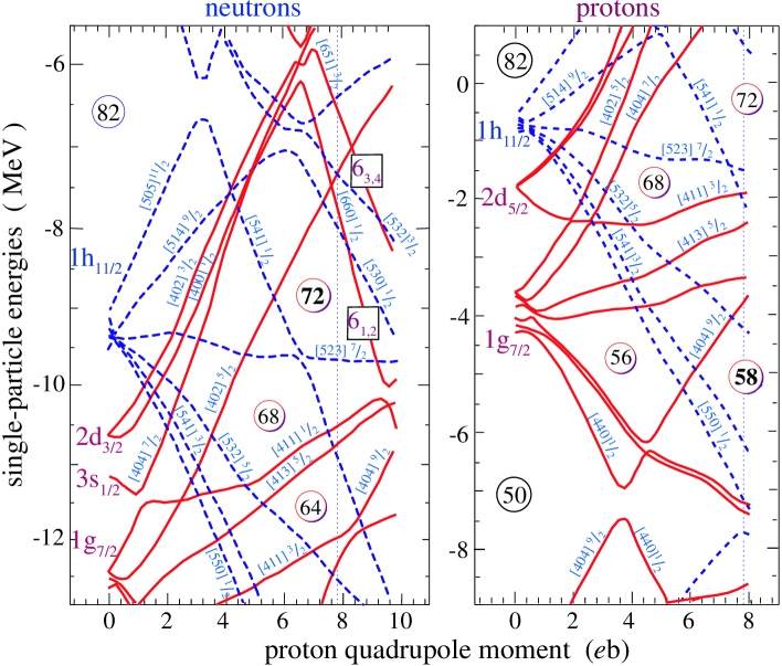
Figure 1: (color online) Single-particle energies for neutrons (left) and protons (right) in ¹²⁸Ba as a function of the proton quadrupole moment calculated in the HF+SLy4 model. Solid and dashed lines mark positive and negative parity states, respectively. The orbitals are labeled by the asymptotic (Nilsson) quantum numbers $[{\cal N}n_{z}\Lambda]\Omega$ of the dominant component of the s.p. wave function. The neutron intruder orbitals originating from the ${\cal N}$=6 shell are additionally labeled by the main oscillator quantum number and a subscript denoting the position of the orbital within the ${\cal N}$ shell.

For quadrupole moments, the additivity principle was experimentally confirmed in the $A$$\sim$140-150 mass region of superdeformation. It was shown that the quadrupole moments of the SD bands in ¹⁴²Sm 142Sm-exp and ¹⁴⁶Gd 146Gd-exp could be well explained in terms of the ¹⁵²Dy SD core and effective s.p. quadrupole moments of valence (particle and hole) orbits. All of these studies, together with the previous results for moments of inertia NWJ.89 ; AKR.96 and effective alignments Rag.93 ; ALR.98 , strongly suggest that the SD bands in the $A$$\sim$140-150 mass region are excellent examples of an almost undisturbed s.p. motion. This is especially true at rotational frequencies above $\hbar\omega$=0.5 MeV AKR.96 ; ALR.98 where pairing is expected to be of minor importance. (For other excellent examples of an almost undisturbed s.p. motion at high spins, see Refs. AFLR.99 ; SW.05 ; Sto.06 .)

In the mass $A$$\sim$135   ($Z$=58-62) light rare-earth region, large $Z$=58 and $N$=72 shell gaps (see Fig. 1 and Refs. Wyss.88 ; AR.96 ) lead to the existence of rotational structures with characteristics typical of highly deformed and SD bands. These bands were observed up to high and very high spins (see Refs. Ce132-131 ; A130-exp2 and references quoted therein). For example, the yrast SD band in ¹³²Ce extends to $\sim$68$\hbar$, which represents one of the highest spin states ever observed in atomic nuclei Ce132-131 . At such high spins, pairing is expected to play a minor role NWJ.89 ; AR.96 ; A130-exp1 , which is a necessary condition for the additivity principle to hold. In this mass region, experimental studies of the additivity principle were performed in Refs. A130-exp1 ; A130-exp2 . Differential lifetime measurements, free from common systematic errors, were performed for over 15 different nuclei (various isotopes of Ce, Pr, Nd, Pm, and Sm) at high spin within a single experiment A130-exp1 ; A130-exp2 .

There are several notable differences between the $A$$\sim$135 and $A$$\sim$140-150 regions of superdeformation. In particular, the rotational bands in the $A$$\sim$135 region are calculated to correspond to the local energy minima that are characterized by much larger $\gamma$-softness than those in the $A$$\sim$140-150 mass region Wyss.88 ; AR.96 . Thus, one of the main goals of the present manuscript is to find the impact of the $\gamma$-softness on the additivity principle. The second goal is a detailed study of the additivity principle not only for quadrupole moments but also for angular momentum alignments. The present work is the first study where the additivity of relative alignments has been tested within the CHF and CRMF frameworks in a systematic way along with the additivity of quadrupole moments. Some results of this study have been reported in Refs. A130-exp1 ; A130-exp2 .

This paper is organized as follows. The principle of additivity, definitions of physical observables, the way of finding effective s.p. quantities, and details of theoretical calculations are discussed in Sec. II. Analysis of the additivity principle for quadrupole moments and relative alignments, and the discussion of associated theoretical uncertainties are presented in Sec. III. Finally, Sec. IV contains the main conclusions of our work.

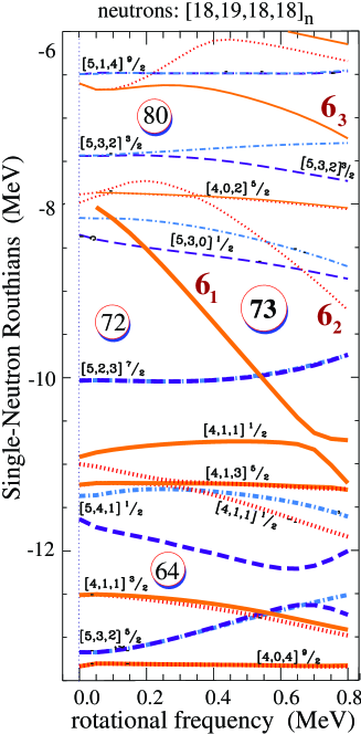
Figure 2: (color online) Neutron s.p. energies (routhians) in the self-consistent rotating potential (CHF+SLy4) as a function of rotational frequency for the core configuration (the lowest highly deformed band of ¹³¹Ce). Occupied (empty) states are denoted by thick (thin) lines. Dotted, solid, dot-dashed, and dashed lines indicate parity and signature quantum numbers $(\pi,r)$=$(+,+i)$, $(+,-i)$, ($-,+i)$, and $(-,-i)$, respectively. The orbitals are also labeled by the asymptotic quantum numbers $[{\cal N}n_{z}\Lambda]\Omega$ of the dominant harmonic oscillator component of the wave function. The neutron intruder orbitals originating from the ${\cal N}$=6 shell are additionally marked. At intermediate rotational frequencies, the lowest intruder level 6₁ becomes occupied and this leads to the presence of the large gap in the spectrum at $N$=73.

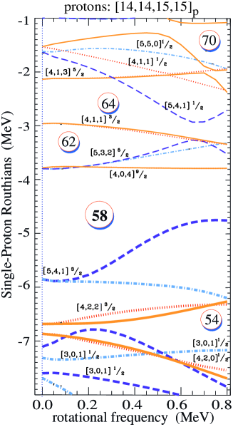
Figure 3: (color online) Similar to Fig. 2 except for proton s.p. states. The large proton $Z$=58 gap in the s.p. spectrum is present at all frequencies considered.

II Theoretical framework

II.1 Definition of observables

Since pairing is neglected in this work, the charge quadrupole moments $Q_{20}$ and $Q_{22}$ are defined microscopically as sums of expectation values of the s.p. quadrupole moment operators $\hat{q}_{20}$ and $\hat{q}_{22}$ of the occupied proton states, i.e.,

$$Q_{20} = \sum_{\mu}\left<\mu|\hat{q}_{20}|\mu\right>,$$ (1)

$$Q_{22} = \sum_{\mu}\left<\mu|\hat{q}_{22}|\mu\right>,$$ (2)

where $\hat{q}_{20}$ and $\hat{q}_{22}$ are defined in three-dimensional Cartesian coordinates as Qdef (conserved signature symmetry is assumed)

$$\hat{q}_{20} = 2z^{2}-x^{2}-y^{2},$$ (3)

$$\hat{q}_{22} = \sqrt{3}(x^{2}-y^{2}).$$ (4)

The factor of $\sqrt{3}$ is included in the definition of $\hat{q}_{22}$ in order to have the following expressions for the total quadrupole moment $Q_{2}$ and the associated Bohr angle $\gamma$:

$$Q_{2} = \sqrt{Q_{20}^{2}+Q_{22}^{2}},$$ (5)

$$\tan(\gamma) = Q_{22}/Q_{20}.$$ (6)

Note that the sums in Eqs. (1–2) run only over proton states. The neutrons, having zero electric charge, do not appear in the sums explicitly, but they influence the charge quadrupole moments indirectly via the quadrupole polarization (deformation changes) induced by occupying/emptying single-neutron states.

It should be noted that with the definitions (1–6), the spherical components of the quadrupole tensor are $Q_{20}$ and $Q_{22}/\sqrt{2}$. This fact is important for the definition of the so-called transition quadrupole moment $Q_{t}$ Retal.82 ; [Ham86a] . This moment gives the measure of the transition strength of the $\Delta I$=2 (stretched) $E2$ radiation in the limit of large deformation and angular momentum, and it is proportional to the component $Q^{\omega}_{22}/\sqrt{2}$ of the spherical quadrupole tensor when the quantization axis coincides with the vector of rotational velocity $\omega$, i.e.,

$$Q^{\omega}_{20} = D^{2}_{0,0}(\psi^{\omega},\theta^{\omega},\phi^{\omega})Q_{20}+\left[D^{2}_{0,2}(\psi^{\omega},\theta^{\omega},\phi^{\omega})+D^{2}_{0,-2}(\psi^{\omega},\theta^{\omega},\phi^{\omega})\right]\frac{Q_{22}}{\sqrt{2}},$$ (7)

$$\frac{Q^{\omega}_{22}}{\sqrt{2}} = D^{2}_{2,0}(\psi^{\omega},\theta^{\omega},\phi^{\omega})Q_{20}+\left[D^{2}_{2,2}(\psi^{\omega},\theta^{\omega},\phi^{\omega})+D^{2}_{2,-2}(\psi^{\omega},\theta^{\omega},\phi^{\omega})\right]\frac{Q_{22}}{\sqrt{2}}.$$ (8)

Here, symbols $D^{\lambda}_{\mu\nu}$ denote the Wigner functions [Var88] , with their arguments $\psi^{\omega},\theta^{\omega},\phi^{\omega}$ being the Euler angles that rotate the $z$ axis (the standard quantization axis for spherical tensors) onto the direction of the angular velocity.

For the cranking axis coinciding with the $y$-axis of the intrinsic system, as is the case for the code HFODD DD.97a ; DD.97b used in the present study, the Euler angles are $\psi$=0, $\theta$=$\pi/2$, and $\phi$=$\pi/2$, which gives:

$$Q^{\omega\parallel{y}}_{20} = -{1\over 2}Q_{20}-\sqrt{{3\over 2}}\frac{Q_{22}}{\sqrt{2}},$$ (9)

$$\frac{Q^{\omega\parallel{y}}_{22}}{\sqrt{2}} = \sqrt{3\over 8}Q_{20}-{1\over 2}\frac{Q_{22}}{\sqrt{2}}.$$ (10)

The second of these equations gives the definition of the transition quadrupole moment used in this work:

$$Q^{\omega\parallel{y}}_{t}=\sqrt{8\over 3}\frac{Q^{\omega\parallel{y}}_{22}}{\sqrt{2}}=Q_{20}-\sqrt{{2\over 3}}\frac{Q_{22}}{\sqrt{2}}.$$ (11)

In order to provide a link to studies that employ the $x$-axis cranking, like, e.g., Refs. Retal.82 ; [Ham86a] and our earlier papers A130-exp1 ; A130-exp2 , we repeat derivations for the Euler angles $\psi$=$\pi/2$, $\theta$=$\pi/2$, $\phi$=$\pi$, which rotate the $z$ axis onto the $x$ axis:

$$Q^{\omega\parallel{x}}_{20} = -{1\over 2}Q_{20}+\sqrt{{3\over 2}}\frac{Q_{22}}{\sqrt{2}},$$ (12)

$$\frac{Q^{\omega\parallel{x}}_{22}}{\sqrt{2}} = -\sqrt{3\over 8}Q_{20}-{1\over 2}\frac{Q_{22}}{\sqrt{2}},$$ (13)

hence

$$Q^{\omega\parallel{x}}_{t}=-\sqrt{8\over 3}\frac{Q^{\omega\parallel{y}}_{22}}{\sqrt{2}}=Q_{20}+\sqrt{{2\over 3}}\frac{Q_{22}}{\sqrt{2}}.$$ (14)

Although definitions (11) and (14) differ by signs of the second terms, values of $Q^{\omega\parallel{y}}_{t}$ and $Q^{\omega\parallel{x}}_{t}$ obtained in self-consistent calculations must be identical because they cannot depend on the direction of the cranking axis. It means that values of $Q_{22}$ obtained in cranking calculations along the $y$ and $x$ axes have opposite signs. In what follows, we employ definition (11) of the transition moment and drop the superscripts that denote the direction of the cranking axis, e.g.,

$$Q_{t} = Q_{20}-\sqrt{{1\over 3}}\,Q_{22},$$ (15)

$$\hat{q}_{t} = \hat{q}_{20}-\sqrt{{1\over 3}}\,\hat{q}_{22}.$$ (16)

Finally, the expectation value of the total angular momentum $J$ (its projection on the cranking axis) is defined as a sum of the expectation values of the s.p. angular momentum operators $\hat{j}_{y}$ of the occupied states

$$J\equiv\langle\hat{J}_{y}\rangle=\sum_{\mu}\left<\mu|\hat{j}_{y}|\mu\right>.$$ (17)

The value of $J$ can be expressed in terms of the total spin $I$ via the cranking relation I.54

$$J=\sqrt{I(I+1)}\approx I+\frac{1}{2}.$$ (18)

II.2 Additivity of effective s.p. observables

For each $k$-configuration defined by occupying a given set of s.p. orbitals and represented by a product state $|k\rangle$, we determine the average value $O(k)=\langle{k}|\hat{O}|k\rangle$ of a s.p. operator $\hat{O}$. We may now designate one of these configurations as a reference, or a core configuration, and determine the relative change $\delta O(k)\equiv O(k)-Q^{\text{core}}$ of the physical observable in the $k$-th configuration with respect to that in the core configuration. The additivity principle stipulates that all these differences can be expressed as sums of individual effective contributions $o^{\text{eff}}_{\alpha}$ coming from s.p. states (enumerated by index $\alpha$), i.e.,

$$O(k)-Q^{\text{core}}\equiv\delta O(k)=\sum_{\alpha}c_{\alpha}(k)o^{\text{eff}}_{\alpha}.$$ (19)

Coefficients $c_{\alpha}$ in Eq. (19) define the s.p. content of the configuration $k$ with respect to the core configuration. Namely,

• $c_{\alpha}(k)=0$ if the state $\alpha$ is not occupied in either of these two configurations, or is occupied in both of them,

• $c_{\alpha}(k)=1$ if $\alpha$ has a particle character (it is occupied in the $k$-th configuration and is not occupied in the core configuration),

• $c_{\alpha}(k)=-1$ if the state $\alpha$ has a hole character (it is not occupied in the $k$-th configuration and is occupied in the core configuration).

In this way, one can label the $k$-th configuration with the set of coefficients $c(k)=\{c_{\alpha}(k),\alpha=1,\dots,m\}$, where $m$ denotes the size of s.p. space considered. The values of $o^{\text{eff}}_{\alpha}$ can be calculated by proceeding step by step from the core configuration to the configurations differing by one particle or one hole, then to the configurations differing by two particles, two holes, or a particle and a hole, and so forth, until the data set is generated which is statistically large enough to provide appreciable precision for $o_{\alpha}^{\text{eff}}$. Had the additivity principle been obeyed exactly, calculations limited to one-particle and one-hole configurations would have sufficed. Since our goal is not only to determine values of $o^{\text{eff}}_{\alpha}$ but actually prove that the additivity principle holds up to a given accuracy, we have to consider a large set of configurations and determine the best values of $o^{\text{eff}}_{\alpha}$ together with their error bars.

In what follows, we consider relative changes in the average quadrupole moments $\delta Q_{20}(k)$ and $\delta Q_{22}(k)$, transition quadrupole moments $\delta Q_{t}(k)$, and total angular momenta $\delta J(k)$ (see Sec. II.1), which are related to the effective one-body expectation values via the additivity principle.

The addition of particle or hole in a specific single-particle orbital $\alpha$ gives rise to a polarization of the system, so the effective s.p. values, $o^{\text{eff}}_{\alpha}$, depend not only on the bare s.p. expectation values, $o^{\text{bare}}_{\alpha}=\left<\hat{o}\right>_{\alpha}$, but also contain polarization contributions. For example, the effective s.p. charge quadrupole moment $q_{20,\alpha}^{\text{eff}}$ can be represented as the sums of bare s.p.  charge quadrupole moments $q_{20,\alpha}^{\text{bare}}=\left<\hat{q}_{20}\right>_{\alpha}$ and polarization contributions $q^{\text{pol}}_{20,\alpha}$:

$$q^{\text{eff}}_{20,\alpha}=q^{\text{bare}}_{20,\alpha}+q^{\text{pol}}_{20,\alpha}.$$ (20)

Therefore, for neutron orbitals, which have vanishing bare charge quadrupole moments, $q^{\text{bare}}_{20,\alpha_{n}}=0$, the effective charge quadrupole moments are solely given by polarization terms:

$$q^{\text{eff}}_{20,\alpha_{n}}=q^{\text{\text{pol}}}_{20,\alpha_{n}}.$$ (21)

II.3 Determination of effective s.p.  observables

Once the averages of physical observables $O(k)$ for the set of $N_{c}$ calculated configurations ($k=1,\dots,N_{c}$) are determined, the effective s.p.  contributions $o^{\text{eff}}_{\alpha}$ (19) are found by means of a multivariate least-square fit (see, e.g., Refs. P-book ; LH-book ). This is done by minimizing the function of $o^{\text{eff}}_{\alpha}$ defined by

$$F\left[o^{\text{eff}}_{\alpha}\right]=\sum_{k=1}^{N_{c}}\left(\delta O(k)-\sum_{\alpha=1}^{m}o_{\alpha}^{\text{eff}}c_{\alpha}(k)\right)^{2}.$$ (22)

Note that the problem is only meaningful when the number of configurations is sufficiently large, $N_{c}>m$. Following the general concept of the least-square method, the partial differentiation with respect to the variables $o^{\text{eff}}_{\alpha}$ yields

$$0 = \frac{1}{2}\frac{\partial}{\partial o_{\alpha}^{\text{eff}}}F\left[o^{\text{eff}}_{\alpha}\right]={}$$ (23)

$$= \sum_{\alpha^{\prime}}\sum_{k}c_{\alpha}(k)c_{\alpha^{\prime}}(k)o^{\text{eff}}_{\alpha^{\prime}}-\sum_{k}\delta O(k)c_{\alpha}(k)=$$

$$= (Bo^{\text{eff}}-a)_{\alpha},$$

where $a_{\alpha}=\sum_{k}\delta O(k)c_{\alpha}(k)=c^{T}\delta O$ and $B=||B_{\alpha\alpha^{\prime}}||=||\sum_{k}c_{\alpha}(k)c_{\alpha^{\prime}}(k)||=c^{T}c$. Solving this equation by inverting the non-singular matrix $B$ gives the solution to the multivariate regression problem:

$$\tilde{o}^{\text{eff}}=B^{-1}a=(c^{T}c)^{-1}c^{T}\delta O.$$ (24)

The fact that $B$ is positive-definite guarantees that the solution $\tilde{o}^{\text{eff}}$ corresponds to a minimum of $F\left[o^{\text{eff}}_{\alpha}\right]$.

In order to estimate the variance, we assume that the first statistical moments of residuals,

$$\epsilon_{O}(k)=\delta O(k)-\sum_{\alpha}c_{\alpha}(k)\tilde{o}_{\alpha}^{\text{eff}},$$ (25)

are zero for all $k=1,...,N_{c}$. Consequently, $\tilde{o}^{\text{eff}}$ can be considered an unbiased estimate of $o^{\text{eff}}$. Furthermore, under the assumption that

$$\text{var}(\epsilon_{O}(k))=\sigma^{2}$$ (26)

for all $k=1,\ldots,N_{c}$, and

$$\text{cov}(\epsilon_{O}(k),\epsilon_{O}(k^{\prime}))=0$$ (27)

for all $\{k,k^{\prime}=1,\ldots,N_{c}|k\neq k^{\prime}\}$, one can define the variance-covariance matrix as $\sigma^{2}B^{-1}=\sigma^{2}(c^{T}c)^{-1}$, for which the unbiased estimate for $\sigma^{2}$ is given by

$$\tilde{\sigma}^{2}=\frac{1}{N_{c}-m}\sum_{k=1}^{N_{c}}\epsilon_{O}(k)^{2}.$$ (28)

Finally, the unbiased estimate for the variance-covariance matrix for $\tilde{o}^{\text{eff}}$ is given by $B^{-1}\sigma^{2}$. In what follows we do not differentiate between notations for variables and their estimates. The least-square procedure described in this section was used to determine the effective s.p. quadrupole moments $\{q_{20,\alpha}^{\text{eff}},q_{22,\alpha}^{\text{eff}},q_{t,\alpha}^{\text{eff}},\alpha=1,...,m\}$ and angular momentum alignments $\{j_{\alpha}^{\text{eff}},\alpha=1,...,m\}$.

II.4 Method of calculations

The CHF calculations were performed using the code HFODD (v1.75) DD.97a ; DD.97b with the interaction SLy4 Cha98 . The accuracy of the harmonic oscillator (HO) expansion depends on the frequencies ($\hbar\omega_{x}$, $\hbar\omega_{y}$, and $\hbar\omega_{z}$) of the oscillator wave functions and the number $M$ of the HO states included in the basis. The basis set includes the lowest $M$ states with energies given by

$$\varepsilon_{n_{x},n_{y},n_{z}}=\hbar\omega_{x}(n_{x}+\frac{1}{2})+\hbar\omega_{y}(n_{y}+\frac{1}{2})+\hbar\omega_{z}(n_{z}+\frac{1}{2}).$$ (29)

An axially symmetric basis ($\omega_{x}=\omega_{y}$) with the deformation $q=\omega_{x}/\omega_{z}=1.81$, oscillator frequency $\hbar\omega_{0}=41A^{-1/3}$ MeV, and value of $M=296$ was used in all the CHF calculations. This basis provides sufficient numerical accuracy for the physical observables of interest Mladen-thesis .

The CRMF calculations were performed using the computer code developed in Refs. KR.89 ; KR.93 ; AKR.96 . An anisotropic three-dimensional harmonic oscillator basis with deformation ($\beta_{0}=0.4,\,\gamma=0^{\circ}$) has been used in the CRMF calculations. All fermionic states below the energy cutoff $E^{\mbox{\scriptsize cut-off}}_{F}\leq 11.5\hbar\omega^{F}_{0}$ and all bosonic states below the energy cutoff $E^{\mbox{\scriptsize cut-off}}_{B}\leq 16.5\hbar\omega^{B}_{0}$ were used in the diagonalization and the matrix inversion. This basis provides sufficient numerical accuracy. The NL1 parametrization of the RMF Lagrangian NL1 has been used in the CRMF calculations. As follows from our previous studies, this parametrization provides reasonable s.p.  energies for nuclei around the valley of $\beta$-stability ALR.98 ; A250 .

II.5 Selection of independent-particle configurations

In both CHF and CRMF calculations, the set of independent-particle configurations in nuclei around ¹³¹Ce was considered. The final sets used in additivity analysis consisted of 183 and 105 configurations in the CHF and CRMF variants, respectively. All ambiguous cases, due to crossings, convergence difficulties, etc., were removed from those sets. Since the CRMF calculations are more time-consuming than the CHF ones, the CRMF set is smaller. Nonetheless, the adopted CRMF set is sufficiently large to provide reliable results. To put things in perspective, in Ref. SDDN.96 , where the CHF analysis of additivity principle in the SD bands of the $A\sim 150$ mass region was carried out, 74 calculated SD configurations were considered.

Every calculated product-state configuration was labeled using the standard notation in terms of parity-signature blocks $\left[N_{+,+i},N_{+,-i},N_{-,+i},N_{-,-i}\right]$, where $N_{\pi,r}$ are the numbers of occupied s.p.  orbitals having parity $\pi$ and signature $r$. In addition, the s.p. states were labeled by the Nilsson quantum numbers and signature $[{\cal N}n_{z}\Lambda]\Omega^{r}$ of the active orbitals at zero frequency. The orbital identification is relatively straightforward when the s.p.  levels do not cross (or cross with a small interaction matrix element), but it can become ambiguous when the crossings with strong mixing occur. In some cases, it was necessary to construct diabatic routhians by removing weak interaction at crossing points. Even with these precautions, a reliable configuration assignment was not always possible; the exceptional cases were excluded from the additivity analysis. Clearly, the likelihood of the occurrence of level crossings is reduced when the s.p. level density is small, e.g., in the vicinity of large shell gaps.

Large deformed energy gaps develop at high rotational velocity for $Z$=58 and $N$=73 (see Figs. 2 and 3). Therefore, the lowest SD band ($\nu i_{13/2}$ band) in ¹³¹Ce is a natural choice for the highly deformed core configuration in the $A$$\sim$130 mass region. The additivity analysis was performed at a large rotational frequency of $\hbar\omega$=0.65 MeV. This choice was dictated by the fact that (i) at this frequency the pairing is already considerably quenched, and (ii) no level crossings appear in the core configuration around this frequency (cf. Figs. 2 and 3). Moreover, at this frequency, the lowest neutron $i_{13/2}$ intruder orbital already appears below the $N$=73 neutron gap (see Fig. 2). The choice of an odd-even core, strongly motivated by its doubly closed character at large deformations/spins, does not impact the additivity scheme, which is insensitive to the selection of the reference system.

The highly deformed core configuration in ¹³¹Ce ([18,19,18,18]${}_{n}\otimes$ [14,14,15,15]_p) has the following orbital structure:

$$\left|{\mbox{\bf core}}\right>=\left|{\mbox{\bf core}}\right>_{\nu} \otimes \left|{\mbox{\bf core}}\right>_{\pi}\equiv$$

$$\begin{array}[]{r}(\nu(1i_{13/2}){\mbox{\bf 6}}_{1}^{-i})\\[-1.0pt] (\nu(1h_{11/2})[523]7/2^{\pm i})^{2}\\[-1.0pt] (\nu(1s_{1/2})[411]1/2^{\pm i})^{2}\\[-1.0pt] (\nu(1g_{7/2})[413]5/2^{\pm i})^{2}\\[-1.0pt] (\nu(2f_{7/2})[541]1/2^{\pm i})^{2}\\[-1.0pt] (\nu(2d_{5/2})[411]3/2^{\pm i})^{2}\\[-1.0pt] (\nu(1h_{11/2})[532]5/2^{\pm i})^{2}\\[-1.0pt] (\nu(1g_{9/2})[404]9/2^{\pm i})^{2}\\[1.0pt] (~{}\cdots~{})\left|{\mbox{\bf 0}}\right>_{\nu}\end{array} \otimes \begin{array}[]{r}(\pi(1g_{9/2})[404]9/2^{\pm i})^{2}\\ (\pi(1h_{11/2})[541]3/2^{\pm i})^{2}\\ (\pi(1g_{7/2})[420]1/2^{\pm i})^{2}\\ (\pi(2d_{5/2})[422]3/2^{\pm i})^{2}\\ (\pi(1h_{11/2})[550]1/2^{\pm i})^{2}\\ (\pi(2p_{1/2})[301]1/2^{\pm i})^{2}\\[1.0pt] (~{}\cdots~{})\left|{\mbox{\bf 0}}\right>_{\pi},\end{array}$$ (46)

where dots denote the deeply bound states and $\left|{\mbox{\bf 0}}\right>_{\nu}$ and $\left|{\mbox{\bf 0}}\right>_{\pi}$ are the neutron and proton vacua, respectively. The spherical subshells from which the deformed s.p.  orbitals emerge (cf. Fig. 1) are indicated in the front of the Nilsson labels.

The Nilsson orbital content of an excited configuration is given in terms of particle and hole excitations with respect to the core configuration through the action of particle/hole operators with quantum labels corresponding to the occupied or emptied Nilsson orbitals. The character of the orbital (particle or hole) is defined by the position of the orbital with respect to the Fermi level of the core configuration. It is clear from Fig. 2 that the neutron states $\nu[523]7/2^{\pm i}$, $\nu[411]1/2^{\pm i}$, $\nu[413]5/2^{\pm i}$, $\nu[541]1/2^{\pm i}$, $\nu[532]5/2^{\pm i}$ and $\nu 6^{-i}_{1}$ have hole character, while $\nu 6^{+i}_{2}$, $\nu 6^{-i}_{3}$, $\nu[530]1/2^{\pm i}$, $\nu[402]5/2^{\pm i}$, $\nu[532]3/2^{\pm i}$, and $\nu[514]9/2^{\pm i}$ have particle character. In a similar way, the proton orbitals $\pi[541]3/2^{\pm i}$, $\pi[422]3/2^{\pm i}$, $\pi[301]1/2^{\pm i}$, and $\pi[420]1/2^{\pm i}$ and $\pi[404]9/2^{\pm i}$ can be viewed as holes, while $\pi[532]5/2^{\pm i}$, $\pi[411]3/2^{\pm i}$, $\pi[541]1/2^{\pm i}$, and $\pi[413]5/2^{\pm}$ have particle character (see Fig. 3).

III Results of the additivity analysis

III.1 Effective charge quadrupole moments $q^{\text{eff}}_{20,\alpha}$

Table 1 contains the values of CHF and CRMF effective s.p. charge quadrupole moments $q^{\text{eff}}_{20,\alpha}$ for a number of s.p. orbitals in the vicinity of the deformed shell gaps at $Z$=58 and $N$=73 (see Figs. 2 and 3). There is an overall excellent agreement between $q_{20,\alpha}^{\text{eff}}$ values for the two mean-field approaches employed. In the majority of cases, the uncertainties are small enough to allow determination of effective moments to two significant digits.

Table 1: Effective s.p.  charge quadrupole moments $q^{\text{eff}}_{20,\alpha}$ (in eb) for the s.p.  orbitals active in the $A$$\sim$130 mass region of high- and superdeformation. Calculations were carried out with CHF+SLy4 and CRMF+NL1 approaches. The bare quadrupole moments $q^{\text{bare}}_{20,\alpha}$ are also shown for CHF+SLy4. Theoretical errors resulting from the multivariate least-square fit are indicated. The results of previous calculations SDDN.96 pertaining to the $A$$\sim$150 mass region are displayed for comparison.

State		CHF+SkP	CHF+SkM*	CHF+SLy4				CRMF+NL1
[${\cal N}n_{z}\Lambda$]$\Omega^{r}$	$p/h$	$q_{20,\alpha}^{\text{eff}}$	$q_{20,\alpha}^{\text{eff}}$	$p/h$	$q^{\text{bare}}_{20,\alpha}$	$q_{20,\alpha}^{\text{eff}}$		$q_{20,\alpha}^{\text{eff}}$
$\nu$ [402]$\frac{5}{2}^{+i}$	$p$	–0.44	–0.38	$p$	0.0	–0.35$\pm$	0.01	–0.26$\pm$	0.01
$\nu$ [402]$\frac{5}{2}^{-i}$	$p$	–0.44	–0.38	$p$	0.0	–0.34$\pm$	0.02	–0.26$\pm$	0.02
$\nu$ [411]$\frac{1}{2}^{+i}$	$h$		–0.18	$h$	0.0	–0.15$\pm$	0.02	–0.11$\pm$	0.02
$\nu$ [411]$\frac{1}{2}^{-i}$	$h$		–0.15	$h$	0.0	–0.12$\pm$	0.01	–0.06$\pm$	0.02
$\nu$ [411]$\frac{3}{2}^{+i}$	$h$			$h$	0.0	–0.15$\pm$	0.04	–0.13$\pm$	0.03
$\nu$ [411]$\frac{3}{2}^{-i}$	$h$			$h$	0.0	–0.11$\pm$	0.05	–0.12$\pm$	0.03
$\nu$ [413]$\frac{5}{2}^{+i}$	$h$	–0.16		$h$	0.0	–0.13$\pm$	0.02	–0.13$\pm$	0.03
$\nu$ [413]$\frac{5}{2}^{-i}$	$h$	–0.13		$h$	0.0	–0.12$\pm$	0.03	–0.11$\pm$	0.02
$\nu$ [523]$\frac{7}{2}^{+i}$				$h$	0.0	0.03$\pm$	0.01	0.05$\pm$	0.01
$\nu$ [523]$\frac{7}{2}^{-i}$				$h$	0.0	0.04$\pm$	0.01	0.01$\pm$	0.02
$\nu$ [530]$\frac{1}{2}^{+i}$				$p$	0.0	0.22$\pm$	0.01	0.17$\pm$	0.01
$\nu$ [530]$\frac{1}{2}^{-i}$				$p$	0.0	0.17$\pm$	0.01	0.19$\pm$	0.01
$\nu$ [532]$\frac{3}{2}^{+i}$				$p$	0.0	0.21$\pm$	0.03	—
$\nu$ [532]$\frac{3}{2}^{-i}$				$p$	0.0	0.17$\pm$	0.03	—
$\nu$ [532]$\frac{5}{2}^{+i}$				$h$	0.0	0.19$\pm$	0.03	0.17$\pm$	0.03
$\nu$ [532]$\frac{5}{2}^{-i}$				$h$	0.0	0.24$\pm$	0.03	0.38$\pm$	0.03
$\nu$ [541]$\frac{1}{2}^{+i}$				$h$	0.0	0.35$\pm$	0.03	0.35$\pm$	0.02
$\nu$ [541]$\frac{1}{2}^{-i}$				$h$	0.0	0.37$\pm$	0.03	0.33$\pm$	0.03
$\nu$ 6${}_{1}^{-i}$				$h$	0.0	0.38$\pm$	0.01	0.40$\pm$	0.01
$\nu$ 6${}_{2}^{+i}$				$p$	0.0	0.36$\pm$	0.01	0.36$\pm$	0.01
$\nu$ 6${}_{3}^{-i}$	$h$	0.43	0.30	$p$	0.0	0.35$\pm$	0.05	—
$\pi$ [301]$\frac{1}{2}^{+i}$	$h$	–0.15	–0.13	$h$	–0.08	0.51$\pm$	0.05	—
$\pi$ [404]$\frac{9}{2}^{+i}$	$p$	–0.30	–0.28	$p$	–0.13	–0.32$\pm$	0.01	–0.37$\pm$	0.01
$\pi$ [404]$\frac{9}{2}^{-i}$	$p$	–0.30	–0.28	$p$	–0.13	–0.32$\pm$	0.01	–0.37$\pm$	0.01
$\pi$ [411]$\frac{3}{2}^{+i}$	$p$	0.11	0.10	$p$	0.06	–0.05$\pm$	0.02	—
$\pi$ [411]$\frac{3}{2}^{-i}$	$p$	0.11	0.10	$p$	0.06	0.00$\pm$	0.01	—
$\pi$ [413]$\frac{5}{2}^{-i}$				$p$	0.06	0.28$\pm$	0.05	—
$\pi$ [422]$\frac{3}{2}^{+i}$				$h$	0.20	0.33$\pm$	0.02	0.33$\pm$	0.03
$\pi$ [422]$\frac{3}{2}^{-i}$				$h$	0.22	0.34$\pm$	0.02	0.28$\pm$	0.02
$\pi$ [532]$\frac{5}{2}^{+i}$				$p$	0.28	0.43$\pm$	0.01	0.41$\pm$	0.02
$\pi$ [532]$\frac{5}{2}^{-i}$				$p$	0.36	0.56$\pm$	0.03	0.54$\pm$	0.03
$\pi$ [541]$\frac{1}{2}^{-i}$				$p$	0.40	0.58$\pm$	0.02	—
$\pi$ [541]$\frac{3}{2}^{+i}$				$h$	0.34	0.50$\pm$	0.01	0.48$\pm$	0.01
$\pi$ [541]$\frac{3}{2}^{-i}$				$h$	0.39	0.57$\pm$	0.01	0.50$\pm$	0.01
$\pi$ [550]$\frac{1}{2}^{-i}$				$h$	0.30	0.49$\pm$	0.05	0.47$\pm$	0.04

The two lowest neutron intruder orbitals 6${}_{1}^{-i}$ and 6${}_{2}^{+i}$ show significant signature splitting, and their effective charge quadrupole moment values differ by more than 5%. The extracted values confirm the general expectations for the polarization effects exerted by the intruder and extruder states FM83 ; CFL83 . The lowest neutron ${\cal N}$=6 orbitals, 6${}_{1}^{-i}$ and 6${}_{2}^{+i}$, have $q_{20,\alpha}^{\text{eff}}\simeq$ 0.37 eb, which indicates that their occupation drives the nucleus towards larger prolate deformation. The third intruder orbital, 6${}_{3}^{-i}$, although calculated with relatively poor statistics, confirms this trend.

The proton $\pi[404]9/2^{\pm i}$ extruder high-$\Omega$ orbitals are oblate-driving; they have large negative values of $q_{20,\alpha}^{\text{eff}}$. Emptying them polarizes the nucleus towards more prolate-deformed shapes. Interestingly, their $q_{20,\alpha}^{\text{eff}}$ values of around $-0.31$ eb are close in magnitude to those of the ${\cal N}$=6 neutron intruders, in line with the findings of Ref. AR.96 that the holes in the proton $g_{9/2}$ orbitals are as important as the particles in the neutron $i_{13/2}$ orbitals in stabilizing the shape at large deformation. Due to their high-$\Omega$ content, the signature splitting of $\pi[404]9/2^{\pm i}$ routhians is extremely small and their $q_{20,\alpha}^{\text{eff}}$ values are practically indistinguishable within error bars.

Our study indicates that proton $h_{11/2}$ states, such as $\pi[541]3/2^{\pm i}$ and $\pi[532]5/2^{\pm i}$ active below and above the $Z$=58 shell gap, respectively, play a significant role in the existence of this island of high deformation. Indeed, Table 1 attributes them to effective charge quadrupole moments in excess of 0.45 eb - very significant values compared with other states listed.

The downsloping orbital $\pi[541]1/2^{-i}$, originating from mixed $\pi f_{7/2}\oplus h_{9/2}$ subshells, carries a large effective charge quadrupole moment of more than 0.5 eb. Although one could expect it to play a role in the formation of large prolate deformation, this state appears too high in energy (above the $Z$=58 shell gap) and would therefore always stay unoccupied in most of the configurations of interest A130-exp1 ; A130-exp2 ; Ce132-131 . On the contrary, the strongly prolate-driving $\pi[550]1/2^{-i}$ orbital carrying $q_{20,\alpha}^{\text{eff}}$$\approx$0.47 eb, is always occupied in the bands of interest.

Table 1 compares the values of $q_{20,\alpha}^{\text{eff}}$ obtained in the present study with those from the additivity analysis of the SD bands in the $A$$\sim$150 region SDDN.96 based on the Skyrme SkP and SkM* energy density functionals. Note that some of the states, which are of particle character in the $A$$\sim$130 region, appear as hole states in the heavier region. For these states, conforming to our definitions of coefficients $c_{\alpha}$ (Sec. II.2), we inverted signs of values shown in Table 1 of Ref. SDDN.96 . With few exceptions, $q_{20,\alpha}^{\text{eff}}$ values are similar in both studies: only for the $\pi[301]1/2^{+i}$ orbital does the difference between $A\sim 130$ and $A\sim 150$ results exceed 0.1 eb. This result strongly suggests that the polarization effects caused by occupying/emptying specific orbitals are mainly due to the general geometric properties of s.p. orbitals and weakly depend on the actual parametrization of the Skyrme energy density functional; minor differences are likely related to interactions between close-lying s.p. states. These observations give strong reasons for combining the two regions into one, and interpreting the entire area of highly and SD rotational states in the mass range $A\sim 128-160$ within the united theoretical framework.

The results for $q_{20,\alpha}^{\text{eff}}$ obtained in CHF+SLy4 and CRMF+NL1 models are indeed very similar (see Table 1). Only for the $\nu[402]5/2^{\pm i}$ and $\nu[532]5/2^{-i}$ orbitals, do the differences between $q_{20,\alpha}^{\text{eff}}$ values come close to 0.1 eb.

Table 1 compares the bare and effective s.p.  charge quadrupole moments obtained in CHF+SLy4. In the majority of cases, these quantities differ drastically, underlying the importance of shape polarization effects. Large differences between bare and effective s.p.  quadrupole moments have also been found in the CHF+SkP and CHF+SkM* calculations in the $A$$\sim$150 region of superdeformation SDDN.96 .

III.2 Effective quadrupole moments $q_{t,\alpha}^{\text{eff}}$ and $q_{22,\alpha}^{\text{eff}}$

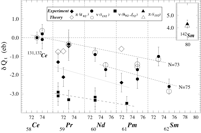
Figure 4: Experimental (closed symbols with error bars) and calculated (CRMF+NL1, open symbols) differential transition quadrupole moments for highly deformed bands in Ce, Pr, Nd, Pm, and Sm isotopes. The experimental data were taken from Refs. A130-exp1 ; A130-exp2 and references quoted therein. The values of $\delta Q_{t}$ for SD band in ¹³²Sm are shown in the inset. Dashed lines are drawn to guide the eye.

Table 2 displays the calculated effective s.p.  transition quadrupole moments $q_{t,\alpha}^{\text{eff}}$, cf. definitions (15–16). Based on the additivity principle, these values can be used to predict the total charge transition moments $Q_{t}(k)$ in highly deformed and SD bands of $A\sim 130$ nuclei:

$$Q_{t}(k)=Q_{t}^{\text{core}}+\sum_{\alpha}c_{\alpha}(k)q_{t,\alpha}^{\text{eff}},$$ (47)

where the calculated CHF+SLy4 value for the core configuration in ¹³¹Cs is

$$Q_{t}^{\text{core}}=7.64\,\mbox{eb}.$$ (48)

Since the total calculated values are less precise than the relative ones which define the effective s.p.  transition quadrupole moments $q_{t,\alpha}^{\text{eff}}$, one may alternatively use in Eq. (47) the measured value Cla96 ,

$$Q_{t}^{\text{core,exp}}=7.4(3)\,\mbox{eb}.$$ (49)

Theoretical estimates of the total charge transition moments $Q_{t}(k)$ allow for predictions of $B(E2)$ values

$$B(E2)(I\rightarrow{I-2},k)=\frac{5}{16\pi}e^{2}\langle I0\,20|I-2\,0\rangle Q^{2}_{t}(k),$$ (50)

and lifetimes NR.96 .

In CHF+SLy4, the uncertainties of $q_{22,\alpha}^{\text{eff}}$ appear to be larger than those for $q_{20,\alpha}^{\text{eff}}$. In CRMF+NL1, however, those uncertainties are similar. This can be traced back to the different $\gamma$-softness of potential energy surfaces in CHF+SLy4 and CRMF+NL1 (see Ref. AR.96 and references quoted therein for the results obtained in different approaches); current analysis revealing large uncertainties for $q_{22,\alpha}^{\text{eff}}$ suggests that the potential energy surfaces are softer (and, thus less localized) in the CHF+SLy4 approach.

Although the values of $q_{22,\alpha}^{\text{eff}}$ are generally much smaller than $q_{20,\alpha}^{\text{eff}}$, large uncertainties in the determination of certain moments $q_{22,\alpha}^{\text{eff}}$ (especially, for $\nu[411]3/2^{\pm i}$, $\nu[532]5/2^{\pm i}$, $\nu 6_{3}^{-i}$, $\pi[301]1/2^{+i}$, and $\pi[550]1/2^{-i}$ orbitals, for which the errors exceed 0.1 eb in the CHF+SLy4 approach) can lead to the deterioration of predicted $q_{t,\alpha}^{\text{eff}}$. On the other hand, in many cases the uncertainties in $q_{22,\alpha}^{\text{eff}}$ are smaller than the experimental error bars; hence, they are less relevant when comparison with experiment is carried out. Currently available experimental data on relative transition quadrupole moments agree reasonably well with the CHF+SLy4 results A130-exp1 ; A130-exp2 .

Table 2 compares $q_{t,\alpha}^{\text{eff}}$ values obtained in CHF+SLy4 and CRMF+NL1 models. The results for proton orbitals are similar in both approaches: the differences between respective $q_{t,\alpha}^{\text{eff}}$ values do not exceed 0.1 eb. Larger differences are seen for the neutrons: for about 50 percent of calculated orbitals ($\nu[402]5/2^{\pm i}$, $\nu[411]1/2^{\pm i}$, $\nu[411]3/2^{+i}$, $\nu[413]5/2^{-i}$, $\nu[530]1/2^{+i}$, and $\nu[532]5/2^{+i}$), the difference between $q_{t,\alpha}^{\text{eff}}$ values in CHF+SLy4 and CRMF+NL1 exceeds 0.1 eb. Interaction (mixing) between those close-lying states (see Fig. 2), predicted differently in the two approaches, is the most likely reason for the deviations seen.

The results of CHF+SLy4 were compared with experimental transition moments in Refs. A130-exp1 ; A130-exp2 . Here, we show in Fig. 4 a comparison between CRMF+NL1 and experiment for the relative transition quadrupole moments $\delta Q_{t}(k)$ in different highly deformed and SD bands in nuclei with $Z$=57-62 involving $i_{13/2}$ neutrons and/or $g_{9/2}$ proton holes. The agreement between experiment and theory is quite remarkable with all the experimental trends discussed in Refs. A130-exp1 ; A130-exp2 well reproduced by calculations. One should note that the CRMF and CHF results are close to each other. The general pattern of decreasing $Q_{t}$ with increasing $Z$ and $N$ is consistent with the general expectation that as one adds particles above a deformed shell gap, the deformation-stabilizing effect of the gap is diminished. This trend continues until a new “magic” deformed number is reached. Such a situation occurs when going from ¹³²Ce towards $Z$=62 and $N$=80 (¹⁴²Sm), where a large jump in transition quadrupole moment takes place marking the point at which it becomes energetically favorable to fill the high-$j$ $\pi i_{13/2}$ and $\nu j_{15/2}$ orbitals responsible for the existence of the $A\sim 142$ SD island.

It is gratifying to see that CRMF+NL1 reproduces the value of $Q_{t}$ in ¹⁴²Sm based on the ¹³¹Ce core (see inset in Fig. 4). Earlier on, it was demonstrated in Refs. A130-exp1 ; A130-exp2 ; 142Sm-exp that this $Q_{t}$ value can be also reproduced within CHF using either a ¹³¹Ce or a ¹⁵²Dy core.

Table 2: Effective s.p.  charge quadrupole moments $q_{20,\alpha}^{\text{eff}}$ and $q_{22,\alpha}^{\text{eff}}$ as well as the transition quadrupole moments $q_{t,\alpha}^{\text{eff}}$ (all in eb) calculated in CHF+SLy4 and CRMF+NL1.

State	CSHF + SLy4						CRMF + NL1
[${\cal N}n_{z}\Lambda$]$\Omega^{r}$	$q_{20,\alpha}^{\text{eff}}$		$q_{22,\alpha}^{\text{eff}}$		$q_{t,\alpha}^{\text{eff}}$		$q_{20,\alpha}^{\text{eff}}$		$q_{22,\alpha}^{\text{eff}}$		$q_{t,\alpha}^{\text{eff}}$
$\nu$[402]$\frac{5}{2}^{+i}$	–0.35$\pm$	0.01	0.14$\pm$	0.06	–0.04$\pm$	0.04	–0.26$\pm$	0.02	–0.02$\pm$	0.01	–0.25$\pm$	0.02
$\nu$[402]$\frac{5}{2}^{-i}$	–0.34$\pm$	0.02	0.08$\pm$	0.08	–0.38$\pm$	0.05	–0.26$\pm$	0.02	–0.07$\pm$	0.02	–0.22$\pm$	0.03
$\nu$[411]$\frac{1}{2}^{+i}$	–0.15$\pm$	0.02	–0.24$\pm$	0.10	–0.01$\pm$	0.06	–0.11$\pm$	0.02	0.09$\pm$	0.02	–0.16$\pm$	0.02
$\nu$[411]$\frac{1}{2}^{-i}$	–0.12$\pm$	0.01	0.06$\pm$	0.06	–0.16$\pm$	0.04	–0.06$\pm$	0.02	–0.17$\pm$	0.02	0.04$\pm$	0.02
$\nu$[411]$\frac{3}{2}^{+i}$	–0.15$\pm$	0.04	0.20$\pm$	0.20	–0.26$\pm$	0.12	–0.13$\pm$	0.03	–0.02$\pm$	0.03	–0.11$\pm$	0.03
$\nu$[411]$\frac{3}{2}^{-i}$	–0.11$\pm$	0.05	–0.05$\pm$	0.24	–0.08$\pm$	0.15	–0.12$\pm$	0.03	0.02$\pm$	0.03	–0.12$\pm$	0.03
$\nu$[413]$\frac{5}{2}^{+i}$	–0.13$\pm$	0.02	–0.05$\pm$	0.10	–0.10$\pm$	0.06	–0.13$\pm$	0.03	–0.04$\pm$	0.03	–0.10$\pm$	0.03
$\nu$[413]$\frac{5}{2}^{-i}$	–0.12$\pm$	0.03	–0.12$\pm$	0.13	–0.05$\pm$	0.08	–0.11$\pm$	0.02	0.15$\pm$	0.03	–0.20$\pm$	0.03
$\nu$[523]$\frac{7}{2}^{+i}$	0.03$\pm$	0.01	–0.00$\pm$	0.05	0.03$\pm$	0.03	0.05$\pm$	0.01	0.00$\pm$	0.01	0.04$\pm$	0.01
$\nu$[523]$\frac{7}{2}^{-i}$	0.04$\pm$	0.01	–0.01$\pm$	0.05	0.05$\pm$	0.03	0.01$\pm$	0.02	–0.00$\pm$	0.02	0.01$\pm$	0.02
$\nu$[530]$\frac{1}{2}^{+i}$	0.22$\pm$	0.01	–0.21$\pm$	0.05	0.34$\pm$	0.03	0.17$\pm$	0.01	–0.09$\pm$	0.01	0.22$\pm$	0.01
$\nu$[530]$\frac{1}{2}^{-i}$	0.17$\pm$	0.01	–0.01$\pm$	0.05	0.18$\pm$	0.03	0.19$\pm$	0.01	0.10$\pm$	0.01	0.13$\pm$	0.01
$\nu$[532]$\frac{3}{2}^{+i}$	0.21$\pm$	0.03	0.21$\pm$	0.13	0.09$\pm$	0.08	—		—		—
$\nu$[532]$\frac{3}{2}^{-i}$	0.17$\pm$	0.03	0.03$\pm$	0.13	0.15$\pm$	0.08	—		—		—
$\nu$[532]$\frac{5}{2}^{+i}$	0.19$\pm$	0.03	–0.08$\pm$	0.20	0.24$\pm$	0.12	0.17$\pm$	0.03	–0.02$\pm$	0.03	0.18$\pm$	0.03
$\nu$[532]$\frac{5}{2}^{-i}$	0.24$\pm$	0.03	–0.01$\pm$	0.20	0.25$\pm$	0.12	0.38$\pm$	0.03	0.00$\pm$	0.03	0.38$\pm$	0.03
$\nu$[541]$\frac{1}{2}^{+i}$	0.35$\pm$	0.03	–0.04$\pm$	0.13	0.38$\pm$	0.08	0.35$\pm$	0.02	–0.00$\pm$	0.02	0.35$\pm$	0.03
$\nu$[541]$\frac{1}{2}^{-i}$	0.37$\pm$	0.03	0.01$\pm$	0.14	0.36$\pm$	0.08	0.33$\pm$	0.03	0.04$\pm$	0.03	0.30$\pm$	0.03
$\nu$ 6${}_{1}^{-i}$	0.38$\pm$	0.01	0.21$\pm$	0.03	0.26$\pm$	0.02	0.40$\pm$	0.01	0.12$\pm$	0.01	0.33$\pm$	0.01
$\nu$ 6${}_{2}^{+i}$	0.36$\pm$	0.01	–0.01$\pm$	0.04	0.37$\pm$	0.03	0.36$\pm$	0.01	–0.01$\pm$	0.01	0.37$\pm$	0.01
$\nu$ 6${}_{3}^{-i}$	0.35$\pm$	0.05	–0.06$\pm$	0.22	0.38$\pm$	0.13	—		—		—
$\pi$[301]$\frac{1}{2}^{+i}$	0.51$\pm$	0.05	–0.10$\pm$	0.24	0.57$\pm$	0.14	—		—		—
$\pi$[404]$\frac{9}{2}^{+i}$	–0.32$\pm$	0.01	0.10$\pm$	0.04	–0.38$\pm$	0.02	–0.37$\pm$	0.01	0.02$\pm$	0.01	–0.38$\pm$	0.01
$\pi$[404]$\frac{9}{2}^{-i}$	–0.32$\pm$	0.01	0.09$\pm$	0.04	–0.37$\pm$	0.02	–0.37$\pm$	0.01	0.02$\pm$	0.01	–0.38$\pm$	0.01
$\pi$[411]$\frac{3}{2}^{+i}$	–0.05$\pm$	0.02	0.10$\pm$	0.07	–0.10$\pm$	0.05	—		—		—
$\pi$[411]$\frac{3}{2}^{-i}$	0.00$\pm$	0.01	–0.22$\pm$	0.07	0.12$\pm$	0.04	—		—		—
$\pi$[422]$\frac{3}{2}^{+i}$	0.33$\pm$	0.02	–0.27$\pm$	0.10	0.48$\pm$	0.06	0.33$\pm$	0.03	–0.13$\pm$	0.02	0.40$\pm$	0.03
$\pi$[422]$\frac{3}{2}^{-i}$	0.34$\pm$	0.02	0.14$\pm$	0.10	0.25$\pm$	0.06	0.28$\pm$	0.02	0.16$\pm$	0.02	0.19$\pm$	0.02
$\pi$[532]$\frac{5}{2}^{+i}$	0.43$\pm$	0.01	–0.05$\pm$	0.05	–0.46$\pm$	0.03	0.41$\pm$	0.02	–0.04$\pm$	0.01	0.43$\pm$	0.02
$\pi$[532]$\frac{5}{2}^{-i}$	0.56$\pm$	0.03	–0.07$\pm$	0.09	0.60$\pm$	0.05	0.54$\pm$	0.03	0.05$\pm$	0.03	0.51$\pm$	0.04
$\pi$[541]$\frac{1}{2}^{-i}$	0.58$\pm$	0.02	–0.01$\pm$	0.10	0.59$\pm$	0.06	—		—		—
$\pi$[541]$\frac{3}{2}^{+i}$	0.50$\pm$	0.01	–0.05$\pm$	0.06	0.52$\pm$	0.04	0.48$\pm$	0.01	–0.10$\pm$	0.01	0.54$\pm$	0.01
$\pi$[541]$\frac{3}{2}^{-i}$	0.57$\pm$	0.01	–0.12$\pm$	0.04	0.63$\pm$	0.03	0.50$\pm$	0.01	–0.10$\pm$	0.01	0.56$\pm$	0.01
$\pi$[550]$\frac{1}{2}^{-i}$	0.49$\pm$	0.05	–0.06$\pm$	0.22	0.52$\pm$	0.14	0.47$\pm$	0.04	–0.02$\pm$	0.04	0.48$\pm$	0.04

Table 3: Effective s.p.  angular momentum alignments $j^{\text{eff}}_{\alpha}$ (in $\hbar$) of the active orbitals calculated in CHF+SLy4 and CRMF+NL1. In the second column, the bare s.p.  angular momenta $j^{\text{bare}}_{\alpha}$, calculated with CHF+SLy4 are also shown.

State	CHF+SLy4			CRMF+NL1
[${\cal N}n_{z}\Lambda$]$\Omega^{r}$	$j^{\text{bare}}_{\alpha}$	$j^{\text{eff}}_{\alpha}$		$j^{\text{eff}}_{\alpha}$
$\nu$ [402]$\frac{5}{2}^{+i}$	$-$0.528	0.58$\pm$	0.14	0.47$\pm$	0.15
$\nu$ [402]$\frac{5}{2}^{-i}$	$-$0.493	0.51$\pm$	0.20	0.38$\pm$	0.26
$\nu$ [411]$\frac{1}{2}^{+i}$	$-$0.411	0.67$\pm$	0.24	0.64$\pm$	0.17
$\nu$ [411]$\frac{1}{2}^{-i}$	$-$0.380	0.40$\pm$	0.15	0.09$\pm$	0.16
$\nu$ [411]$\frac{3}{2}^{+i}$	$-$0.092	1.72$\pm$	0.46	1.35$\pm$	0.29
$\nu$ [411]$\frac{3}{2}^{-i}$	$-$0.077	0.56$\pm$	0.57	1.08$\pm$	0.29
$\nu$ [413]$\frac{5}{2}^{+i}$	$-$0.316	$-$0.10$\pm$	0.23	0.44$\pm$	0.27
$\nu$ [413]$\frac{5}{2}^{-i}$	$-$0.428	0.12$\pm$	0.30	0.14$\pm$	0.26
$\nu$ [523]$\frac{7}{2}^{+i}$	$-$0.908	$-$1.10$\pm$	0.10	$-$1.24$\pm$	0.12
$\nu$ [523]$\frac{7}{2}^{-i}$	$-$0.974	$-$1.19$\pm$	0.12	$-$0.92$\pm$	0.18
$\nu$ [530]$\frac{1}{2}^{+i}$	$-$1.548	1.19$\pm$	0.11	1.86$\pm$	0.09
$\nu$ [530]$\frac{1}{2}^{-i}$	$-$0.564	0.88$\pm$	0.11	0.93$\pm$	0.10
$\nu$ [532]$\frac{3}{2}^{+i}$	$-$0.171	$-$0.34$\pm$	0.30	—
$\nu$ [532]$\frac{3}{2}^{-i}$	$-$0.835	0.44$\pm$	0.31	—
$\nu$ [532]$\frac{5}{2}^{+i}$	$-$0.331	$-$0.89$\pm$	0.46	$-$0.95$\pm$	0.29
$\nu$ [532]$\frac{5}{2}^{-i}$	$-$0.417	$-$1.06$\pm$	0.46	$-$1.29$\pm$	0.30
$\nu$ [541]$\frac{1}{2}^{+i}$	$-$1.793	0.92$\pm$	0.31	0.95$\pm$	0.25
$\nu$ [541]$\frac{1}{2}^{-i}$	$-$0.466	0.89$\pm$	0.32	$-$0.34$\pm$	0.28
$\nu$ 6${}_{1}^{-i}$	$-$4.840	4.78$\pm$	0.08	4.59$\pm$	0.08
$\nu$ 6${}_{2}^{+i}$	$-$4.031	3.42$\pm$	0.11	3.15$\pm$	0.10
$\nu$ 6${}_{3}^{-i}$	$-$2.662	0.77$\pm$	0.50	—
$\pi$ [301]$\frac{1}{2}^{+i}$	$-$0.432	1.23$\pm$	0.55	—
$\pi$ [404]$\frac{9}{2}^{+i}$	$-$0.719	$-$0.00$\pm$	0.09	0.09$\pm$	0.09
$\pi$ [404]$\frac{9}{2}^{-i}$	$-$0.719	$-$0.00$\pm$	0.09	0.11$\pm$	0.09
$\pi$ [411]$\frac{3}{2}^{+i}$	$-$0.249	0.81$\pm$	0.18	—
$\pi$ [411]$\frac{3}{2}^{-i}$	$-$0.062	0.65$\pm$	0.16	—
$\pi$ [413]$\frac{5}{2}^{-i}$	$-$0.539	$-$1.52$\pm$	0.53	—
$\pi$ [422]$\frac{3}{2}^{+i}$	$-$0.315	$-$0.19$\pm$	0.25	$-$0.21$\pm$	0.27
$\pi$ [422]$\frac{3}{2}^{-i}$	$-$0.510	$-$0.84$\pm$	0.23	$-$0.38$\pm$	0.24
$\pi$ [532]$\frac{5}{2}^{+i}$	$-$0.253	$-$0.90$\pm$	0.13	$-$1.11$\pm$	0.16
$\pi$ [532]$\frac{5}{2}^{-i}$	$-$0.022	$-$0.67$\pm$	0.20	—
$\pi$ [541]$\frac{1}{2}^{-i}$	$-$0.944	1.75$\pm$	0.23	—
$\pi$ [541]$\frac{3}{2}^{+i}$	$-$1.743	1.57$\pm$	0.13	1.18$\pm$	0.11
$\pi$ [541]$\frac{3}{2}^{-i}$	$-$0.057	$-$0.54$\pm$	0.10	$-$0.48$\pm$	0.11
$\pi$ [550]$\frac{1}{2}^{-i}$	$-$2.819	2.99$\pm$	0.52	2.86$\pm$	0.40

III.3 Effective angular momenta $j^{\text{eff}}_{\alpha}$ (s.p. alignments)

In this section, we evaluate and interpret the effective s.p. contributions to the total angular momentum. Table 3 displays effective s.p.  angular momenta $j^{\text{eff}}_{\alpha}$ for the s.p. orbitals of interest. The relative uncertainties in calculated $j^{\text{eff}}_{\alpha}$ values are on average larger than those for effective s.p.  quadrupole moments. This is due to the fact that, on the mean field level, polarization effects pertaining to the angular momentum are more complex than those for quadrupole moments: they involve not only shape changes but also the variations of time-odd mean fields DD.95 ; AR.00 ; VALR.05 . For eight proton states calculated in both approaches, the mean uncertainties are $0.19\hbar$ and $0.18\hbar$ in CHF+SLy4 and CRMF+NL1, respectively. The same holds also for the set of 18 neutron states, where the average uncertainties are $0.25\hbar$ and $0.20\hbar$ in CHF+SLy4 and CRMF+NL1, respectively.

Table 3 also compares CHF+SLy4 expectation values of the s.p.  angular momentum $j^{\text{bare}}_{\alpha}=\left<\hat{j}\right>_{\alpha}$ with their effective counterparts $j^{\text{eff}}_{\alpha}$. It is seen that these two quantities differ considerably. As discussed in Ref. AR.00 , this is due to both shape polarization and time-odd mean-field effects. It is also important to remember that, unlike the cranked Nilsson scheme, in self-consistent models the expectation value of the projection of the s.p.  angular momentum on the rotation axis $j^{\text{bare}}_{\alpha}$ cannot be extracted from the slope of its s.p.  routhian versus rotation frequency Gal.94 .

Our results indicate that the additivity principle for angular momentum alignment does not work as precisely as it does for quadrupole moments. This conclusion is in line with a similar analysis in the $A\sim 60$ region of superdeformation D.98 ; A6080 . A configuration assignment based on relative alignments depends on how accurately these alignments can be predicted. For example, the application of effective (relative) alignment method in the $A\sim 140-150$ region of superdeformation requires an accuracy in the prediction of relative angular momenta on the level of $\sim 0.3\hbar$ and $\sim 0.5\hbar$ for non-intruder and intruder orbitals, respectively Rag.93 ; BHN.95 ; ALR.98 . In the highly deformed and SD nuclei from the $A\sim 60-80$ mass region, these requirements for accuracy are somewhat relaxed (see Refs. ARR.99 ; AF.05 ). We expect that in the $A\sim 130$ region, the relative alignments should be predicted with a precision similar to that in the $A\sim 140-150$ region. However, for a number of orbitals (for example, $\nu[411]3/2^{\pm i}$, $\nu[532]5/2^{\pm i}$, $\nu 6_{3}^{-i}$, $\pi[301]1/2^{+i}$, $\pi[413]5/2^{-i}$, $\pi[550]1/2^{-i}$), the calculated uncertainties in $j^{\text{eff}}_{\alpha}$ are close to $0.5\hbar$, and this probably prevents reliable assignments based on the additivity principle for the configurations involving these orbitals. The situation becomes even more uncertain if several orbitals with high uncertainties in $j^{\text{eff}}_{\alpha}$ are occupied.

Let us also remark that while theory provides effective alignments at a fixed rotational frequency, relative alignments extracted from experimental data may show appreciable frequency dependence (see for instance Ref. D.98 ). Therefore, for reliable configuration assignments, measured relative alignments should be compared with calculated ones over a wide frequency range.

III.4 Variance and distribution of residuals

One of the main outcomes of this study is the set of effective s.p.  moments $q_{20,\alpha}^{\text{eff}}$, $q_{22,\alpha}^{\text{eff}}$, $q_{t,\alpha}^{\text{eff}}$, and alignments $j_{\alpha}^{\text{eff}}$. The quality of the additivity principle can be assessed by studying the distribution of first moments of residuals (25), i.e., differences between the self-consistently calculated values of physical observables and those obtained from the additivity principle. For instance, for the quadrupole moment $Q_{20}$, the quantity of interest is

$$\Delta Q_{20}=\sum_{\alpha}{c_{\alpha}(k)q_{20,\alpha}^{\text{eff}}}-\delta Q_{20}(k).$$ (51)

Deviations $\Delta Q_{22}$, $\Delta Q_{t}$, and $\Delta J$ are given by similar expressions. Figures 5 and 6 show distributions of these deviations. The quality of the additivity principle for $Q_{20}$ is shown in the top two panels of Fig. 5. In the CHF model, the majority of $\Delta Q_{20}$ values (more than 97.8% of the total number) fall comfortably within the interval of $\pm$0.1 eb. This corresponds to a relative distribution width of about 1.3%. In CRMF, the distribution is even narrower, with more than 90% of $\Delta Q_{20}$ values falling within the $\pm$0.05 eb interval, or less than 0.7% of the total value.

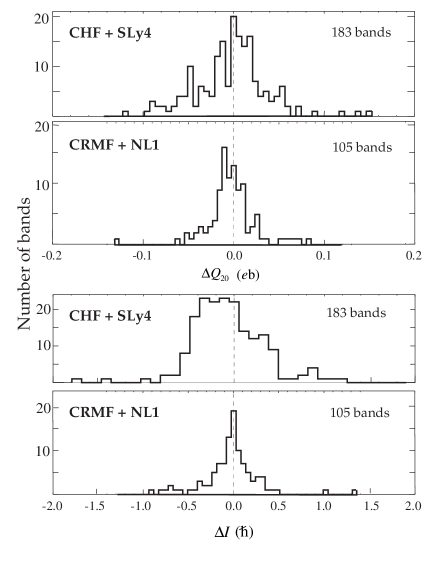
Figure 5: Histogram of differences between self-consistent values obtained in CHF and CRMF and those given by the additivity formula [see e.g. Eq. (51)]. The results for $Q_{20}$ are shown in the two upper panels and those for the total angular momentum are displayed in the two lower panels.

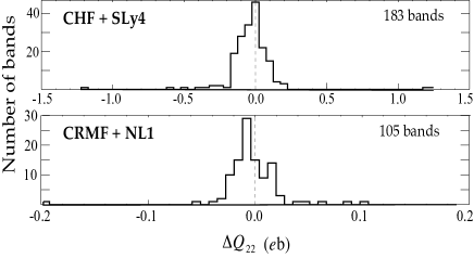
Figure 6: Similar to Fig. 5 except for $Q_{22}$.

The results for the total angular momentum are shown in the bottom panels of Fig. 5. In CRMF, the distribution of deviations is very narrow, with only 10% of the cases differing by more than $\pm\hbar/2$. The CHF histogram is somewhat wider, but more than 90% of deviations fall within the $\pm\hbar/2$ interval. Taking into consideration that the experimental spins of highly deformed and SD bands are often assigned with uncertainties that are multiples of $\hbar$, our results give considerable encouragement for theoretical interpretations based on the method of relative (effective) alignments Rag.93 ; BHN.95 ; ALR.98 .

In CHF and CRMF, the distributions of deviations of charge quadrupole moments $Q_{22}$ (Fig. 6) are relatively narrow. Again, for CRMF, nearly 95% of deviations fall within $\pm$0.025 eb, and 98% fall within $\pm$0.1 eb. For CHF, the distribution of deviations is somewhat wider, with more than 90% of deviations falling within the $\pm$0.2 eb interval.

We interpret these results as a strong indication that the additivity principle works fairly well in self-consistent cranked theories. While distributions of deviations in $Q_{20}$ and $Q_{22}$ are rather similar in the CHF+SLy4 and CRMF+NL1 models (see top of Fig. 5 and Fig. 6), deviations in angular momentum differ between these two approaches. Considering that (i) the uncertainties in $j_{\alpha}^{\text{eff}}$ are similar in both methods (Sec. III.3), and (ii) shape polarization effects are not that different (Sec. III.2), one can conclude that the observed difference is due to the polarization of time-odd mean fields. However, the detailed investigation of this effect is beyond the scope of this study.

IV Conclusions

The additivity principle in highly and SD rotational bands of the $A\sim 130$ mass region has been studied within the cranked Hartree+Fock theory based on the SLy4 energy density functional and the cranked relativistic mean-field theory with the NL1 Lagrangian. The main results can be summarized as follows:

• The two sets of effective s.p. charge quadrupole moments $q_{20}^{\text{eff}}$ and $q_{22}^{\text{eff}}$, transition quadrupole moments $q_{t}^{\text{eff}}$, and effective angular momenta $j^{\text{eff}}$ have been produced. This rich output allows for an easy and simple determination of transition quadrupole moments $Q_{t}$ in highly deformed and SD bands in the $A\sim 130$ mass region. In some cases, configuration assignments based on the relative (effective) alignment method can be done based on the calculated values of effective angular momenta $j^{\text{eff}}$ (see, however, Sec. III.3).

• Our statistical analysis of distributions of residuals confirms that the additivity principle is well fulfilled in the self-consistent approaches that properly take into account polarization effects.

• The contribution from the triaxial degree of freedom to the transition quadrupole moment is usually small, but it cannot be ignored when aiming at a quantitative reproduction of experimental data. The average magnitude of $q_{22}^{\text{eff}}$ values is greater in the CHF+SLy4 model than in CRHF+NL1, thus suggesting that the potential energy surfaces produced in the former model are more $\gamma$-soft.

• For the majority of s.p.  orbitals, there is a considerable difference between the effective and bare expectation values of one-body operators. This indicates the importance of polarization effects (shape polarization for quadrupole moments and the shape and time-odd-mean-field polarization for angular momentum alignment).

• With very few exceptions, there is a great deal of consistency between CHF and CRMF results for the effective s.p. moments and alignments.

So far, the additivity principle has been investigated only for highly deformed or SD bands in the $A$$\sim$130-150 mass region. It would be interesting to extend such studies to other high spin structures. The most promising candidates are: (i) terminating bands in the $A\sim 110$ mass region characterized by very weak pairing and appreciable $\gamma$-softness AFLR.99 , and (ii) SD rotational bands in the $A\sim 60$ and $A\sim 80$ mass regions of superdeformation A6080 . Work along these lines is in progress.

V Acknowledgements

Our study was inspired by the experimental work of Laird et al. A130-exp1 . Stimulating discussions with Mark Riley are gratefully acknowledged. The work was supported in part by the U.S. Department of Energy under Contract Nos. DE-FG02-96ER40963 (University of Tennessee), DE-AC05-00OR22725 with UT-Battelle, LLC (Oak Ridge National Laboratory), and DE-FG05-87ER40361 (Joint Institute for Heavy Ion Research), and DE-FG02-07ER41459 (Mississippi State University); by the Latvian Scientific Council (grant No. 05.1724); by the Polish Ministry of Science; by the Academy of Finland and University of Jyväskylä within the FIDIPRO programme; and by the European Union Social Fund and the research program Pythagoras II - EPEAEK II, under project 80861.

References

- (1) I. Ragnarsson, Phys. Lett. B 264, 5 (1991).
- (2) G. de France, C. Baktash, B. Haas, and W. Nazarewicz, Phys. Rev. C 53, R1070 (1996).
- (3) L. B. Karlsson, I. Ragnarsson, and S. Åberg, Phys. Lett. B 416, 16 (1998).
- (4) J. Zhang, Y. Sun, L. L. Riedinger, and M. Guidry, Phys. Rev. C 58, 868 (1998).
- (5) W. Satuła, J. Dobaczewski, J. Dudek, and W. Nazarewicz, Phys. Rev. Lett. 77 5182 (1996).
- (6) S. Åberg, L.-O. Jönsson, L. B. Karlsson, and I. Ragnarsson, Z. Phys. A 358, 268 (1997).
- (7) L. B. Karlsson, I. Ragnarsson, and S. Åberg, Nucl. Phys. A 639, 654 (1998).
- (8) A. V. Afanasjev, G. Lalazissis, and P. Ring, Nucl. Phys. A 634, 395 (1998)
- (9) G. Hackman, R. V. F. Janssens, E. F. Moore, D. Nisius, I. Ahmad, M. P. Carpenter, S. M. Fischer, T. L. Khoo, T. Lauritsen, and P. Reiter, Phys. Lett. B 416, 268 (1998).
- (10) S. T. Clark, G. Hackman, R. V. F. Janssens, R. M. Clark, P. Fallon, S. N. Floor, G. J. Lane, A. O. Macchiavelli, J. Norris, S. J. Sanders, and C. E. Svensson, Phys. Rev. Lett. 87, 172503 (2001).
- (11) W. Nazarewicz, R. Wyss, and A. Johnson, Nucl. Phys. A 503, 285 (1989).
- (12) A. V. Afanasjev, J. König, and P. Ring, Nucl. Phys. A 608, 107 (1996).
- (13) I. Ragnarsson, Nucl. Phys. A 557, 167c (1993).
- (14) A. V. Afanasjev, D. B. Fossan, G. J. Lane, and I. Ragnarsson, Phys. Rep. 322, 1 (1999).
- (15) W. Satuła and R. Wyss, Rep. Prog. Phys. 68, 131 (2005).
- (16) G. Stoitcheva, W. Satuła, W. Nazarewicz, D.J. Dean, M. Zalewski, and H. Zduńczuk, Phys. Rev. C 73, 061304(R) (2006).
- (17) R. Wyss, J. Nyberg, A. Johnson, R. Bengtsson, and W. Nazarewicz, Phys. Lett. B 215, 211 (1988).
- (18) A. V. Afanasjev and I. Ragnarsson, Nucl. Phys. A 608, 176 (1996).
- (19) E. S. Paul, P. T. W. Choy, C. Andreoiu, A. J. Boston, A. O. Evans, C. Fox, S. Gros, P. J. Nolan, G. Rainovski, J. A. Sampson, H. C. Scraggs, A. Walker, D. E. Appelbe, D. T. Joss, J. Simpson, J. Gizon, A. Astier, N. Buforn, A. Prévost, N. Redon, O. Stézowski, B. M. Nyakó, D. Sohler, J. Timár, L. Zolnai, D. Bazzacco, S. Lunardi, C. M. Petrache, P. Bednarszyk, D. Curien, N. Kintz, and I. Ragnarsson, Phys. Rev. C 71, 054309 (2005).
- (20) M. A. Riley, R. W. Laird, F. G. Kondev, D. J. Hartley, D. E. Archer, T. B. Brown, R. M. Clark, M. Devlin, P. Fallon, I. M. Hibbert, D. T. Joss, D. R. LaFosse, P. J. Nolan, N. J. O’Brien, E. S. Paul, J. Pfohl, D. G. Sarantites, R. K. Sheline, S. L. Shepherd, J. Simpson, R. Wadsworth, M. T. Matev, A. V. Afanasjev, J. Dobaczewski, G. A. Lalazissis, W. Nazarewicz, and W. Satuła, Acta Phys. Polonica B 32, 2683 (2001).
- (21) R. W. Laird, F. G. Kondev, M. A. Riley, D. E. Archer, T. B. Brown, R. M. Clark, M. Devlin, P. Fallon, D. J. Hartley, I. M. Hibbert, D. T. Joss, D. R. LaFosse, P. J. Nolan, N. J. O’Brien, E. S. Paul, J. Pfohl, D. G. Sarantites, R. K. Sheline, S. L. Shepherd, J. Simpson, R. Wadsworth, M. T. Matev, A. V. Afanasjev, J. Dobaczewski, G. A. Lalazissis, W. Nazarewicz, and W. Satuła, Phys. Rev. Lett. 88, 152501 (2002).
- (22) J. Dobaczewski and P. Olbratowski, Comp. Phys. Comm. 158, 158 (2004).
- (23) P. Ring, A. Hayashi, K. Hara, H. Emling, and E. Grosse, Phys. Lett. 110B, 423 (1982).
- (24) I. Hamamoto and Zheng Xing, Phys. Scr. 33, 210 (1986).
- (25) D.A Varshalovitch, A.N. Moskalev, and V.K. Kersonskii, Quantum Theory of Angular Momentum (World Scientific, Singapore, 1988).
- (26) J. Dobaczewski and J. Dudek, Comput. Phys. Commun. 102, 166 (1997).
- (27) J. Dobaczewski and J. Dudek, Comput. Phys. Commun. 102, 183 (1997).
- (28) D. R. Inglis, Phys. Rev. 96, 1059 (1954).
- (29) P. R. Bevington, Data Reduction and Error Analysis for the Physical Sciences, (McGraw-Hill Publ. Co., New York, 1969).
- (30) C. H. Lawson and R. J. Hanson, Solving Least Squares Problems, (Prentice-Hall, New York, 1974).
- (31) E. Chabanat, P. Bonche, P. Haensel, J. Meyer, and F. Schaeffer, Nucl. Phys. A 635, 231 (1998).
- (32) Mladen Matev, Self-Consistent Description of Rotational Properties of Highly Deformed States in Atomic Nuclei Far From Stability, PhD thesis, University of Tennessee, 2003.
- (33) W. Koepf and P. Ring, Nucl. Phys. A 493, 61 (1989)
- (34) J. König, and P. Ring, Phys. Rev. Lett. 71, 3079 (1993).
- (35) P.-G. Reinhard, M. Rufa, J. Maruhn, W. Greiner, and J. Friedrich, Z. Phys. A 323, 13 (1986)
- (36) A. V. Afanasjev, T. L. Khoo, S. Frauendorf, G. A. Lalazissis, and I. Ahmad, Phys. Rev. C 67, 024309 (2003).
- (37) S. Frauendorf and F. R. May, Phys. Lett. B 125, 245 (1983).
- (38) Y.S. Chen, S. Frauendorf, and G.A. Leander, Phys. Rev. C 28, 2437 (1983).
- (39) R.M. Clark, I.Y. Lee, P. Fallon, D.T. Joss, S.J. Asztalos, J.A. Becker, L. Bernstein, B. Cederwall, M.A. Deleplanque, R.M. Diamond, L.P. Farris, K. Hauschild, W.H. Kelly, A.O. Macchiavelli, P.J. Nolan, N. O’Brien, A.T. Semple, F.S. Stephens, and R. Wadsworth, Phys. Rev. Lett. 76, 3510 (1996).
- (40) W. Nazarewicz and I. Ragnarsson, Nuclear Deformations, in Handbook of Nuclear Properties, ed. by D.N. Poenaru and W. Greiner, (Clarendon Press, Oxford), 1996, p. 80.
- (41) J. Dobaczewski and J. Dudek, Phys. Rev. C 52, 1827 (1995).
- (42) A. V. Afanasjev and P. Ring, Phys. Rev. C 62, 031302(R) (2000).
- (43) D. Vretenar, A. V. Afanasjev, G. A. Lalazissis, and P. Ring, Phys. Rep. 409, 101 (2005).
- (44) B. Gall, P. Bonche, J. Dobaczewski, H. Flocard, and P.-H. Heenen, Z. Phys. A 348, 189 (1994).
- (45) J. Dobaczewski, Nuclear Structure’98, AIP Conf. Proc. 481, edited by C. Baktash (American Institute of Physics, New York, 1999), p. 315; nucl-th/9811043.
- (46) J. Dobaczewski, W. Satuła, W. Nazarewicz, and C. Baktash, to be published.
- (47) C. Baktash, B. Haas, and W. Nazarewicz, Ann. Rev. Nucl. Part. Sc. 45, 485 (1995).
- (48) A. V. Afanasjev, I. Ragnarsson, and P. Ring, Phys. Rev. C 59, 3166 (1999).
- (49) A. V. Afanasjev and S. Frauendorf, Phys. Rev. C 71, 064318 (2005).