Stieltjes like functions and inverse problems for systems with Schrödinger operator

Abstract.

A class of scalar Stieltjes like functions is realized as linear-fractional transformations of transfer functions of conservative systems based on a Schrödinger operator $T_{h}$ in $L_{2}[a,+\infty)$ with a non-selfadjoint boundary condition. In particular it is shown that any Stieltjes function of this class can be realized in the unique way so that the main operator ${\mathbb{A}}$ of a system is an accretive $(*)$-extension of a Schrödinger operator $T_{h}$. We derive formulas that restore the system uniquely and allow to find the exact value of a non-real parameter $h$ in the definition of $T_{h}$ as well as a real parameter $\mu$ that appears in the construction of the elements of the realizing system. An elaborate investigation of these formulas shows the dynamics of the restored parameters $h$ and $\mu$ in terms of the changing free term $\gamma$ from the integral representation of the realizable function. It turns out that the parametric equations for the restored parameter $h$ represent different circles whose centers and radii are determined by the realizable function. Similarly, the behavior of the restored parameter $\mu$ are described by hyperbolas.

1. Introduction

Realizations of different classes of holomorphic operator-valued functions in the open right half-plane, unit circle, and upper half-plane, as well as inverse spectral problems, play an important role in the spectral analysis of non-self-adjoint operators, interpolation problems, and system theory. The literature on realization theory is too extensive to be discussed exhaustively in this note. We refer, however, to [2], [3], [7], [8], [9], [11], [12], [18], [24], [28] and the literature therein. A class of Herglotz-Nevanlinna functions is a rich source for many types of realization problems. An operator-valued function $V(z)$ acting on a finite-dimensional Hilbert space $E$ belongs to the class of operator-valued Herglotz-Nevanlinna functions if it is holomorphic on ${{\mathbb{C}}\setminus{\mathbb{R}}}$, if it is symmetric with respect to the real axis, i.e., $V(z)^{*}=V(\bar{z})$, $z\in{{\mathbb{C}}\setminus{\mathbb{R}}}$, and if it satisfies the positivity condition

$${\rm Im\,}V(z)\geq 0,\quad z\in{\mathbb{C}}_{+}.$$

It is well known (see e.g. [16], [17]) that operator-valued Herglotz-Nevanlinna functions admit the following integral representation:

(1.1) $$V(z)=Q+Lz+\int_{{\mathbb{R}}}\left(\frac{1}{t-z}-\frac{t}{1+t^{2}}\right)\,dG(t),\quad z\in{{\mathbb{C}}\setminus{\mathbb{R}}},$$

where $Q=Q^{*}$, $L\geq 0$, and $G(t)$ is a nondecreasing operator-valued function on ${\mathbb{R}}$ with values in the class of nonnegative operators in $E$ such that

(1.2) $$\int_{{\mathbb{R}}}\frac{\left(dG(t)x,x\right)_{E}}{1+t^{2}}<\infty,\quad x\in E.$$

The realization of a selected class of Herglotz-Nevanlinna functions is provided by a linear conservative system $\Theta$ of the form

(1.3) $$\left\{\begin{array}[]{l}({\mathbb{A}}-zI)x=KJ\varphi_{-}\\ \varphi_{+}=\varphi_{-}-2iK^{*}x\end{array}\right.$$

or

(1.4) $$\Theta=\left(\begin{array}[]{ccc}{\mathbb{A}}&K&J\\ {\mathcal{H}}_{+}\subset{\mathcal{H}}\subset{\mathcal{H}}_{-}&&E\\ \end{array}\right).$$

In this system ${\mathbb{A}}$, the main operator of the system, is a so-called ($*$)-extension, which is a bounded linear operator from ${\mathcal{H}}_{+}$ into ${\mathcal{H}}_{-}$, where ${\mathcal{H}}_{+}\subset{\mathcal{H}}\subset{\mathcal{H}}_{-}$ is a rigged Hilbert space. Moreover, $K$ is a bounded linear operator from the finite-dimensional Hilbert space $E$ into ${\mathcal{H}}_{-}$, while $J=J^{*}=J^{-1}$ is acting on $E$, are such that ${\rm Im\,}{\mathbb{A}}=KJK^{*}$. Also, $\varphi_{-}\in E$ is an input vector, $\varphi_{+}\in E$ is an output vector, and $x\in{\mathcal{H}}_{+}$ is a vector of the state space of the system $\Theta$. The system described by (1.3)-(1.4) is called a rigged canonical system of the Livšic type [22] or the Brodskiĭ-Livšic rigged operator colligation, cf., e.g. [11], [12], [13]. The operator-valued function

(1.5) $$W_{\Theta}(z)=I-2iK^{*}({\mathbb{A}}-zI)^{-1}KJ$$

is a transfer function (or characteristic function) of the system $\Theta$. It was shown in [11] that an operator-valued function $V(z)$ acting on a Hilbert space $E$ of the form (1.1) can be represented and realized in the form

(1.6) $$V(z)=i[W_{\Theta}(z)+I]^{-1}[W_{\Theta}(z)-I]=K^{*}({\mathbb{A}}_{R}-zI)^{-1}K,$$

where $W_{\Theta}(z)$ is a transfer function of some canonical scattering ($J=I$) system $\Theta$, and where the “real part” ${\mathbb{A}}_{R}={\frac{1}{2}}({\mathbb{A}}+{\mathbb{A}}^{*})$ of ${\mathbb{A}}$ satisfies ${\mathbb{A}}_{R}\supset A$ if and only if the function $V(z)$ in (1.1) satisfies the following two conditions:

(1.7) $$\left\{\begin{array}[]{l}L=0,\\ Qx=\int_{{\mathbb{R}}}\frac{t}{1+t^{2}}\,dG(t)x\quad\mbox{when}\quad\int_{{\mathbb{R}}}\left(dG(t)x,x\right)_{E}<\infty.\end{array}\right.$$

In the current paper we are going to focus on an important subclass of Herglotz-Nevanlinna functions, the so called Stieltjes like functions that also includes Stieltjes functions. In Section 4 we specify a subclass of realizable Stieltjes operator-functions and show that any member of this subclass can be realized by a system of the form (1.4) whose main operator ${\mathbb{A}}$ is accretive.

In Section 5 we introduce a class of Stieltjes like scalar functions. Then we rely on the general realization results developed in Section 4 (see also [15]) to restore a system $\Theta$ of the form (1.4) containing the Schrödinger operator in $L_{2}[a,+\infty)$ with non-self-adjoint boundary conditions

$$\left\{\begin{array}[]{l}T_{h}y=-y^{\prime\prime}+q(x)y\\ y^{\prime}(a)=hy(a)\\ \end{array}\right.,\quad\left(q(x)=\overline{q(x)},\,{\rm Im\,}h\neq 0\right).$$

We show that if a non-decreasing function $\sigma(t)$ is the spectral distribution function of positive self-adjoint boundary value problem

$$\left\{\begin{array}[]{l}A_{\theta}y=-y^{\prime\prime}+q(x)y\\ y^{\prime}(a)=\theta y(a)\end{array}\right.$$

and satisfies conditions

$$\int\limits_{0}^{\infty}d\sigma(t)=\infty,\quad\int\limits_{0}^{\infty}\frac{d\sigma(t)}{1+t}<\infty,$$

then for every real $\gamma$ a Stieltjes like function

$$V(z)=\gamma+\int\limits_{0}^{\infty}\frac{d\sigma(t)}{t-z}$$

can be realized in the unique way as a $V_{\Theta}(z)$ function of a rigged canonical system $\Theta$ containing some Schrödinger operator $T_{h}$. In particular, it is shown that for every $\gamma\geq 0$ a Stieltjes function $V(z)$ with integral representation above can be realized by a system $\Theta$ whose main operator ${\mathbb{A}}$ is an accretive $(*)$-extension of a Schrödinger operator $T_{h}$.

On top of the general realization results, Section 5 provides the reader with formulas that allow to find the exact value of a non-real parameter $h$ in the definition of $T_{h}$ of the realizing system $\Theta$. Similar investigation is presented in Section 6 to describe the real parameter $\mu$ that appears in the construction of the elements of the realizing system. A detailed study of these formulas shows the dynamics of the restored parameters $h$ and $\mu$ in terms of a changing free term $\gamma$ in the integral representation of $V(z)$ above. It will be shown and graphically presented that the parametric equations for the restored parameter $h$ represent different circles whose centers and radii are completely determined by the function $V(z)$. Similarly, the behavior of the restored parameter $\mu$ are described by hyperbolas.

2. Some preliminaries

For a pair of Hilbert spaces ${\mathcal{H}}_{1}$, ${\mathcal{H}}_{2}$ we denote by $[{\mathcal{H}}_{1},{\mathcal{H}}_{2}]$ the set of all bounded linear operators from ${\mathcal{H}}_{1}$ to ${\mathcal{H}}_{2}$. Let $A$ be a closed, densely defined, symmetric operator in a Hilbert space ${\mathcal{H}}$ with inner product $(f,g),f,g\in{\mathcal{H}}$. Consider the rigged Hilbert space

$${\mathcal{H}}_{+}\subset{\mathcal{H}}\subset{\mathcal{H}}_{-},$$

where ${\mathcal{H}}_{+}=D(A^{*})$ and

$$(f,g)_{+}=(f,g)+(A^{*}f,A^{*}g),\;\;f,g\in D(A^{*}).$$

Note that identifying the space conjugate to ${\mathcal{H}}_{\pm}$ with ${\mathcal{H}}_{\mp}$, we get that if ${\mathbb{A}}\in[{\mathcal{H}}_{+},{\mathcal{H}}_{-}]$ then ${\mathbb{A}}^{*}\in[{\mathcal{H}}_{+},{\mathcal{H}}_{-}].$

Definition 2.1.

An operator ${\mathbb{A}}\in[{\mathcal{H}}_{+},{\mathcal{H}}_{-}]$ is called a self-adjoint bi-extension of a symmetric operator $A$ if ${\mathbb{A}}={\mathbb{A}}^{*}$, ${\mathbb{A}}\supset A$, and the operator

$$\widehat{A}f={\mathbb{A}}f,\;f\in D(\widehat{A})=\{f\in{\mathcal{H}}_{+}:{\mathbb{A}}f\in{\mathcal{H}}\}$$

is self-adjoint in ${\mathcal{H}}$.

The operator $\widehat{A}$ in the above definition is called a quasi-kernel of a self-adjoint bi-extension ${\mathbb{A}}$ (see [27]) .

Definition 2.2.

An operator ${\mathbb{A}}\in[{\mathcal{H}}_{+},{\mathcal{H}}_{-}]$ is called a ($*$)-extension (or correct bi-extension) of an operator $T$ (with non-empty set $\rho(T)$ of regular points) if

$${\mathbb{A}}\supset T\supset A,{\mathbb{A}}^{*}\supset T^{*}\supset A$$

and the operator ${\mathbb{A}}_{R}=\frac{1}{2}({\mathbb{A}}+{\mathbb{A}}^{*})$ is a self-adjoint bi-extension of an operator $A$.

The existence, description, and analog of von Neumann’s formulas for self-adjoint bi-extensions and ($*$)-extensions were discussed in [27] (see also [4], [5], [11]). For instance, if $\Phi$ is an isometric operator from the defect subspace ${\mathfrak{N}}_{i}$ of the symmetric operator $A$ onto the defect subspace ${\mathfrak{N}}_{-i}$, then the formulas below establish a one-to one correspondence between ($*$)-extensions of an operator $T$ and $\Phi$

(2.1) $${\mathbb{A}}f=A^{*}f+iR(\Phi-I)x,\;{\mathbb{A}}^{*}f=A^{*}f+iR(\Phi-I)y,$$

where $x,y\in{\mathfrak{N}}_{i}$ are uniquely determined from the conditions

$$f-(\Phi+I)x\in D(T),\;f-(\Phi+I)y\in D(T^{*})$$

and $R$ is the Riesz-Berezanskii operator of the triplet ${\mathcal{H}}_{+}\subset{\mathcal{H}}\subset{\mathcal{H}}_{-}$ that maps ${\mathcal{H}}_{+}$ isometrically onto ${\mathcal{H}}_{-}$ (see [27]). If the symmetric operator $A$ has deficiency indices $(n,n)$, then formulas (2.1) can be rewritten in the following form

(2.2) $${\mathbb{A}}f=A^{*}f+\sum\limits_{k=1}^{n}{\Delta_{k}(f)V_{k}},\quad{\mathbb{A}}^{*}f=A^{*}f+\sum\limits_{k=1}^{n}{\delta_{k}(f)V_{k}},$$

where $\{V_{j}\}_{1}^{n}\in{\mathcal{H}}_{-}$ is a basis in the subspace $R(\Phi-I){\mathfrak{N}}_{i}$, and $\{\Delta_{k}\}_{1}^{n}$, $\{\delta_{k}\}_{1}^{n}$, are bounded linear functionals on ${\mathcal{H}}_{+}$ with the properties

(2.3) $$\Delta_{k}(f)=0,\;\;\forall f\in D(T),\quad\delta_{k}(f)=0,\;\;\forall f\in D(T^{*}).$$

Let ${\mathcal{H}}=L_{2}[a,+\infty)$ and $l(y)=-y^{\prime\prime}+q(x)y$ where $q$ is a real locally summable function. Suppose that the symmetric operator

(2.4) $$\left\{\begin{array}[]{l}Ay=-y^{\prime\prime}+q(x)y\\ y(a)=y^{\prime}(a)=0\\ \end{array}\right.$$

has deficiency indices (1,1). Let $D^{*}$ be the set of functions locally absolutely continuous together with their first derivatives such that $l(y)\in L_{2}[a,+\infty)$. Consider ${\mathcal{H}}_{+}=D(A^{*})=D^{*}$ with the scalar product

$$(y,z)_{+}=\int_{a}^{\infty}\left(y(x)\overline{z(x)}+l(y)\overline{l(z)}\right)dx,\;\;y,\;z\in D^{*}.$$

Let

$${\mathcal{H}}_{+}\subset L_{2}[a,+\infty)\subset{\mathcal{H}}_{-}$$

be the corresponding triplet of Hilbert spaces. Consider operators

(2.5) $$\left\{\begin{array}[]{l}T_{h}y=l(y)=-y^{\prime\prime}+q(x)y\\ hy(a)-y^{\prime}(a)=0\\ \end{array}\right.,\;\;\left\{\begin{array}[]{l}T^{*}_{h}y=l(y)=-y^{\prime\prime}+q(x)y\\ \overline{h}y(a)-y^{\prime}(a)=0\\ \end{array}\right.,$$

$$\left\{\begin{array}[]{l}\widehat{A}y=l(y)=-y^{\prime\prime}+q(x)y\\ \mu y(a)-y^{\prime}(a)=0\\ \end{array}\right.,\;\;{\rm Im\,}\mu=0.$$

It is well known [1] that $\widehat{A}=\widehat{A^{*}}$. The following theorem was proved in [6].

Theorem 2.3.

The set of all ($*$)-extensions of a non-self-adjoint Schrödinger operator $T_{h}$ of the form (2.5) in $L_{2}[a,+\infty)$ can be represented in the form

(2.6) $$\begin{split}&{\mathbb{A}}y=-y^{\prime\prime}+q(x)y-\frac{1}{\mu-h}\,[y^{\prime}(a)-hy(a)]\,[\mu\delta(x-a)+\delta^{\prime}(x-a)],\\ &{\mathbb{A}}^{*}y=-y^{\prime\prime}+q(x)y-\frac{1}{\mu-\overline{h}}\,[y^{\prime}(a)-\overline{h}y(a)]\,[\mu\delta(x-a)+\delta^{\prime}(x-a)].\end{split}$$

In addition, the formulas (2.6) establish a one-to-one correspondence between the set of all ($*$)-extensions of a Schrödinger operator $T_{h}$ of the form (2.5) and all real numbers $\mu\in[-\infty,+\infty]$.

Definition 2.4.

An operator $T$ with the domain $D(T)$ and $\rho(T)\neq\emptyset$ acting on a Hilbert space ${\mathcal{H}}$ is called accretive if

$${\rm Re\,}(Tf,f)\geq 0,\;\;\forall f\in D(T).$$

Definition 2.5.

An accretive operator $T$ is called [20] $\alpha$-sectorial if there exists a value of $\alpha\in(0,\pi/2)$ such that

$$\cot\alpha\,|{\rm Im\,}(Tf,f)|\leq{\rm Re\,}(Tf,f),\qquad f\in{\mathcal{D}}(T).$$

An accretive operator is called extremal accretive if it is not $\alpha$-sectorial for any $\alpha\in(0,\pi/2)$.

Consider the symmetric operator $A$ of the form (2.4) with defect indices (1,1), generated by the differential operation $l(y)=-y^{\prime\prime}+q(x)y$. Let $\varphi_{k}(x,\lambda)(k=1,2)$ be the solutions of the following Cauchy problems:

$\left\{\begin{array}[]{l}l(\varphi_{1})=\lambda\varphi_{1}\\ \varphi_{1}(a,\lambda)=0\\ \varphi^{\prime}_{1}(a,\lambda)=1\\ \end{array}\right.,$ $\left\{\begin{array}[]{l}l(\varphi_{2})=\lambda\varphi_{2}\\ \varphi_{2}(a,\lambda)=-1\\ \varphi^{\prime}_{2}(a,\lambda)=0\\ \end{array}\right..$

It is well known [1] that there exists a function $m_{\infty}(\lambda)$ (called the Weyl-Titchmarsh function) for which

$$\varphi(x,\lambda)=\varphi_{2}(x,\lambda)+m_{\infty}(\lambda)\varphi_{1}(x,\lambda)$$

belongs to $L_{2}[a,+\infty)$.

Suppose that the symmetric operator $A$ of the form (2.4) with deficiency indices (1,1) is nonnegative, i.e., $(Af,f)\geq 0$ for all $f\in D(A))$. It was shown in [25] that the Schrödinger operator $T_{h}$ of the form (2.5) is accretive if and only if

(2.7) $${\rm Re\,}h\geq-m_{\infty}(-0).$$

For real $h$ such that $h\geq-m_{\infty}(-0)$ we get a description of all nonnegative self-adjoint extensions of an operator $A$. For $h=-m_{\infty}(-0)$ the corresponding operator

(2.8) $$\left\{\begin{array}[]{l}A_{K}\,y=-y^{\prime\prime}+q(x)y\\ y^{\prime}(a)+m_{\infty}(-0)y(a)=0\\ \end{array}\right.$$

is the Kreĭn-von Neumann extension of $A$ and for $h=+\infty$ the corresponding operator

(2.9) $$\left\{\begin{array}[]{l}A_{F}\,y=-y^{\prime\prime}+q(x)y\\ y(a)=0\\ \end{array}\right.$$

is the Friedrichs extension of $A$ (see [25], [6]).

3. Rigged canonical systems with Schrödinger operator

Let ${\mathbb{A}}$ be ($*$) - extension of an operator $T$, i.e.,

$${\mathbb{A}}\supset T\supset A,\quad{\mathbb{A}}^{*}\supset T^{*}\supset A$$

where $A$ is a symmetric operator with deficiency indices ($n,n$) and $D(A)=D(T)\cap D(T^{*})$. In what follows we will only consider the case when the symmetric operator $A$ has dense domain, i.e., $\overline{{\mathcal{D}}(A)}={\mathcal{H}}$.

Definition 3.1.

A system of equations

$$\left\{\begin{array}[]{l}({\mathbb{A}}-zI)x=KJ\varphi_{-}\\ \varphi_{+}=\varphi_{-}-2iK^{*}x\end{array}\right.,$$

or an array

(3.1) $$\Theta=\begin{pmatrix}{\mathbb{A}}&K&\ J\cr{\mathcal{H}}_{+}\subset{\mathcal{H}}\subset{\mathcal{H}}_{-}&&E\cr\end{pmatrix}$$

is called a rigged canonical system of the Livsic type or the Brodskiĭ-Livsic rigged operator colligation if:

1) $E$ is a finite-dimensional Hilbert space with scalar product $(\cdot,\cdot)_{E}$ and the operator $J$ in this space satisfies the conditions $J=J^{*}=J^{-1}$,

2) $K\in[E,{\mathcal{H}}_{-}]$,

3) ${\rm Im\,}{\mathbb{A}}=KJK^{*},$ where $K^{*}\in[{\mathcal{H}}_{+},E]$ is the adjoint of $K$.

In the definition above $\varphi_{-}\in E$ stands for an input vector, $\varphi_{+}\in E$ is an output vector, and $x$ is a state space vector in ${\mathcal{H}}$. An operator ${\mathbb{A}}$ is called a main operator of the system $\Theta$, $J$ is a direction operator, and $K$ is a channel operator. An operator-valued function

(3.2) $$W_{\Theta}(\lambda)=I-2iK^{*}({\mathbb{A}}-\lambda I)^{-1}KJ$$

defined on the set $\rho(T)$ of regular points of an operator $T$ is called the transfer function (characteristic function) of the system $\Theta$, i.e., $\varphi_{+}=W_{\Theta}(\lambda)\varphi_{-}$. It is known [25],[27] that any $(*)$-extension ${\mathbb{A}}$ of an operator $T$ ($A^{*}\supset T\supset A)$, where $A$ is a symmetric operator with deficiency indices $(n,n)$ $(n<\infty)$, $D(A)=D(T)\cap D(T^{*})$, can be included as a main operator of some rigged canonical system with ${\rm dim\,}E<\infty$ and invertible channel operator $K$.

It was also established [25], [27] that

(3.3) $$V_{\Theta}(\lambda)=K^{*}({\rm Re\,}{\mathbb{A}}-\lambda I)^{-1}K$$

is a Herglotz-Nevanlinna operator-valued function acting on a Hilbert space $E$, satisfying the following relation for $\lambda\in\rho(T),\;{\rm Im\,}\lambda\neq 0$

(3.4) $$V_{\Theta}(\lambda)=i[W_{\Theta}(\lambda)-I][W_{\Theta}(\lambda)+I]^{-1}J.$$

Alternatively,

(3.5) $$W_{\Theta}(\lambda) =(I+iV_{\Theta}(\lambda)J)^{-1}(I-iV_{\Theta}(\lambda)J)$$

$$=(I-iV_{\Theta}(\lambda)J)(I+iV_{\Theta}(\lambda)J)^{-1}.$$

Let us recall (see [27], [6]) that a symmetric operator with dense domain ${\mathcal{D}}(A)$ is called prime if there is no reducing, nontrivial invariant subspace on which $A$ induces a self-adjoint operator. It was established in [26] that a symmetric operator $A$ is prime if and only if

(3.6) $$\mathop{c.l.s.}\limits_{\lambda\neq\overline{\lambda}}{\mathfrak{N}}_{\lambda}={\mathcal{H}}.$$

We call a rigged canonical system of the form (3.1) prime if

$$\mathop{c.l.s.}\limits_{\lambda\neq\bar{\lambda},\,\lambda\in\rho(T)}{\mathfrak{N}}_{\lambda}={\mathcal{H}}.$$

One easily verifies that if system $\Theta$ is prime, then a symmetric operator $A$ of the system is prime as well.

The following theorem [6] establishes the connection between two rigged canonical systems with equal transfer functions.

Theorem 3.2.

Let $\Theta_{1}=\begin{pmatrix}{\mathbb{A}}_{1}&K_{1}&J\cr{\mathcal{H}}_{+1}\subset{\mathcal{H}}_{1}\subset{\mathcal{H}}_{-1}&&E\cr\end{pmatrix}$ and
$\Theta_{2}=\begin{pmatrix}{\mathbb{A}}_{2}&K_{2}&J\cr{\mathcal{H}}_{+2}\subset{\mathcal{H}}_{2}\subset{\mathcal{H}}_{-2}&&E\cr\end{pmatrix}$ be two prime rigged canonical systems of the Livsic type with

(3.7) $$\begin{split}&{\mathbb{A}}_{1}\supset T_{1}\supset A_{1},\quad{\mathbb{A}}_{1}^{*}\supset T_{1}^{*}\supset A_{1},\\ &{\mathbb{A}}_{2}\supset T_{2}\supset A_{2},\quad{\mathbb{A}}_{2}^{*}\supset T_{2}^{*}\supset A_{2},\end{split}$$

and such that $A_{1}$ and $A_{2}$ have finite and equal defect indices.

If

(3.8) $$W_{\Theta_{1}}(\lambda)=W_{\Theta_{2}}(\lambda),$$

then there exists an isometric operator $U$ from ${\mathcal{H}}_{1}$ onto ${\mathcal{H}}_{2}$ such that $U_{+}=U|_{{\mathcal{H}}_{+1}}$ is an isometry from ${\mathcal{H}}_{+1}$ onto ${\mathcal{H}}_{+2}$, $U_{-}^{*}=U_{+}^{*}$ is an isometry from ${\mathcal{H}}_{-1}$ onto ${\mathcal{H}}_{-2}$, and

(3.9) $$UT_{1}=T_{2}U,\quad{\mathbb{A}}_{2}=U_{-}{\mathbb{A}}_{1}U_{+}^{-1},\quad U_{-}K_{1}=K_{2}.$$

Corollary 3.3.

Let $\Theta_{1}$ and $\Theta_{2}$ be the two prime systems from the statement of theorem 3.2. Then the mapping $U$ described in the conclusion of the theorem is unique.

Proof.

First let us make an observation that if $\Theta=\begin{pmatrix}{\mathbb{A}}&K&J\cr{\mathcal{H}}_{+}\subset{\mathcal{H}}\subset{\mathcal{H}}_{-}&&E\cr\end{pmatrix}$ is a prime rigged canonical system such that $U_{-}{\mathbb{A}}={\mathbb{A}}U_{+}$ and $U_{-}K=K$, where $U$ is an isometry mapping described in theorem 3.2, then $U=I$. Indeed, it is well known [27] that

(3.10) $$({\rm Re\,}{\mathbb{A}}-\lambda I)^{-1}KE={\mathfrak{N}}_{\lambda}.$$

We have

$$U({\rm Re\,}{\mathbb{A}}-\lambda I)^{-1}K e=U_{+}({\rm Re\,}{\mathbb{A}}-\lambda I)^{-1}Ke=({\rm Re\,}{\mathbb{A}}-\lambda I)^{-1}U_{-}Ke$$

$$=({\rm Re\,}{\mathbb{A}}-\lambda I)^{-1}Ke,\qquad\forall e\in E,\;\lambda\neq\bar{\lambda}.$$

Combining the above equation with (3.6) and (3.10) we obtain $U=I$.

Now let $\Theta_{1}$ and $\Theta_{2}$ be the two prime systems from the statement of theorem 3.2. Suppose there are two isometric mappings $U_{1}$ and $U_{2}$ guaranteed by theorem 3.2. Then the relations

$${\mathbb{A}}_{2}=U_{-,1}{\mathbb{A}}_{1}U_{+,1}^{-1},\quad U_{-,1}K_{1}=K_{2},\quad{\mathbb{A}}_{2}=U_{-,2}{\mathbb{A}}_{1}U_{+,2}^{-1},\quad U_{-,2}K_{1}=K_{2},$$

lead to

$${\mathbb{A}}_{1}U_{+,1}^{-1}U_{+,2}=U_{-,1}^{-1}U_{-,2}{\mathbb{A}}_{1},\quad U_{-,1}^{-1}U_{-,2}K=K.$$

Since $\Theta_{1}$ is prime then $U^{-1}_{1}U_{2}=I$ and hence $U_{1}=U_{2}$. This proves the uniqueness of $U$. ∎

Now we shall construct a rigged canonical system based on a non-self-adjoint Schrödinger operator. One can easily check that the ($*$)-extension

$${\mathbb{A}}y=-y^{\prime\prime}+q(x)y-\frac{1}{\mu-h}\,[y^{\prime}(a)-hy(a)]\,[\mu\delta(x-a)+\delta^{\prime}(x-a)],\;\;{\rm Im\,}h>0$$

of the non-self-adjoint Schrödinger operator $T_{h}$ of the form (2.5) satisfies the condition

(3.11) $${\rm Im\,}{\mathbb{A}}=\frac{{\mathbb{A}}-{\mathbb{A}}^{*}}{2i}=(.,g)g,$$

where

(3.12) $$g=\frac{({\rm Im\,}h)^{\frac{1}{2}}}{|\mu-h|}\,[\mu\delta(x-a)+\delta^{\prime}(x-a)]$$

and $\delta(x-a),\delta^{\prime}(x)$ are the delta-function and its derivative at the point a. Moreover,

(3.13) $$(y,g)=\frac{({\rm Im\,}h)^{\frac{1}{2}}}{|\mu-h|}\ [\mu y(a)-y^{\prime}(a)],$$

where

$$y\in{\mathcal{H}}_{+},g\in{\mathcal{H}}_{-},{\mathcal{H}}_{+}\subset L_{2}(a,+\infty)\subset{\mathcal{H}}_{-}$$

and the triplet of Hilbert spaces is as discussed in theorem 2.3. Let $E={\mathbb{C}}$, $K{c}=cg\;(c\in{\mathbb{C}})$. It is clear that

(3.14) $$K^{*}y=(y,g),\quad y\in{\mathcal{H}}_{+}$$

and ${\rm Im\,}{\mathbb{A}}=KK^{*}.$ Therefore, the array

(3.15) $$\Theta=\begin{pmatrix}{\mathbb{A}}&K&1\cr{\mathcal{H}}_{+}\subset L_{2}[a,+\infty)\subset{\mathcal{H}}_{-}&&{\mathbb{C}}\cr\end{pmatrix}$$

is a rigged canonical system with the main operator ${\mathbb{A}}$ of the form (2.6), the direction operator $J=1$ and the channel operator $K$ of the form (3.14). Our next logical step is finding the transfer function of (3.15). It was shown in [6] that

(3.16) $$W_{\Theta}(\lambda)=\frac{\mu-h}{\mu-\overline{h}}\,\,\frac{m_{\infty}(\lambda)+\overline{h}}{m_{\infty}(\lambda)+h},$$

and

(3.17) $$V_{\Theta}(\lambda)=\frac{\left(m_{\infty}(\lambda)+\mu\right){\rm Im\,}h}{\left(\mu-{\rm Re\,}h\right)m_{\infty}(\lambda)+\mu{\rm Re\,}h-|h|^{2}}.$$

4. Realization of Stieltjes functions

Let $E$ be a finite-dimensional Hilbert space. The scalar versions of the following definition can be found in [19].

Definition 4.1.

We will call an operator-valued Herglotz-Nevanlinna function $V(z)\in[E,E]$ by a Stieltjes function if $V(z)$ admits the following integral representation

(4.1) $$V(z)=\gamma+\int\limits_{0}^{\infty}\frac{dG(t)}{t-z},$$

where $\gamma\geq 0$ and $G(t)$ is a non-decreasing on $[0,+\infty)$ operator-valued function such that

$$\int\limits^{\infty}_{0}\frac{(dG(t)e,e)_{E}}{1+t}<\infty,\quad\forall e\in E.$$

Alternatively (see [19]) an operator-valued function $V(z)$ is Stieltjes if it is holomorphic in $\operatorname{Ext}[0,+\infty)$ and

(4.2) $$\frac{{\rm Im\,}[zV(z)]}{{\rm Im\,}z}\geq 0.$$

The theorem 4.2 below was stated in [14], [15] and we present its proof for the convenience of a reader.

Theorem 4.2.

Let $\Theta$ be a prime system of the form (3.1). Then an operator-valued function $V_{\Theta}(z)$ defined by (3.3), (3.4) is a Stieltjes function if and only if the main operator $\mathbb{A}$ of the system $\Theta$ is accretive.

Proof.

Let us assume first that $\mathbb{A}$ is an accretive operator, i.e. $({\rm Re\,}{\mathbb{A}}x,x)\geq 0$, for all $x\in{\mathcal{H}}_{+}$. Let $\{z_{k}\}$ ($k=1,...,n$) be a sequence of non-real complex numbers and $h_{k}$ be a sequence of vectors in $E$. Let us denote

(4.3) $$Kh_{k}=\delta_{k},\quad x_{k}=({\rm Re\,}{\mathbb{A}}-z_{k}I)^{-1}\delta_{k},\quad x=\sum_{k=1}^{n}x_{k}.$$

Since $({\rm Re\,}{\mathbb{A}}x,x)\geq 0$, we have

(4.4) $$\sum_{k,l=1}^{n}({\rm Re\,}{\mathbb{A}}x_{k},x_{l})\geq 0.$$

By formal calculations one can have

$${\rm Re\,}{\mathbb{A}}x_{k}=\delta_{k}+z_{k}({\rm Re\,}{\mathbb{A}}-z_{k}I)^{-1}\delta_{k},$$

and

$$\sum_{k,l=1}^{n}({\rm Re\,}{\mathbb{A}}x_{k},x_{l}) =\sum_{k,l=1}^{n}\big{[}(\delta_{k},({\rm Re\,}{\mathbb{A}}-z_{l}I)^{-1}\delta_{l})$$

$$+(z_{k}({\rm Re\,}{\mathbb{A}}-z_{k}I)^{-1}\delta_{k},({\rm Re\,}{\mathbb{A}}-z_{k}I)^{-1}\delta_{l})\big{]}.$$

Using obvious equalities

$$\big{(}({\rm Re\,}{\mathbb{A}}-z_{k}I)^{-1}Kh_{k},Kh_{l}\big{)}=\big{(}V_{\theta}(z_{k})h_{k},h_{l}\big{)}_{E},$$

and

$$\big{(}({\rm Re\,}{\mathbb{A}}-\bar{z}_{l}I)^{-1}({\rm Re\,}{\mathbb{A}}-z_{k}I)^{-1}Kh_{k},Kh_{l}\big{)}=\left(\frac{V_{\theta}(z_{k})-V_{\theta}(\bar{z}_{l})}{z_{k}-\bar{z}_{l}}h_{k},h_{l}\right)_{E},$$

we obtain

(4.5) $$\sum_{k,l=1}^{n}({\rm Re\,}{\mathbb{A}}x_{k},x_{l})=\sum_{k,l=1}^{n}\left(\frac{z_{k}V_{\theta}(z_{k})-\bar{z}_{l}V_{\theta}(\bar{z}_{l})}{z_{k}-\bar{z}_{l}}h_{k},h_{l}\right)_{E}\geq 0.$$

The choice of $z_{k}$ was arbitrary, which means that $V_{\Theta}(z)$ is a Stieltjes function (see [3]).

Now we prove necessity. Since $\Theta$ is a prime system then $A$ is a prime symmetric operator. Then the equivalence of (4.5) and (4.4) implies that $({\rm Re\,}{\mathbb{A}}x,x)\geq 0$ for any $x$ from c.l.s.$\left\{\mathfrak{N}_{z}\right\}$, $z\neq\bar{z}$. As we have already mentioned above, a symmetric operator $A$ with the equal deficiency indices is prime if and only if for all $\lambda\neq\bar{\lambda}$

$$\text{\rm c.l.s.}\left\{\mathfrak{N}_{\lambda}\right\}={\mathcal{H}}.$$

Therefore we can conclude that $({\rm Re\,}{\mathbb{A}}x,x)\geq 0$ for any $x\in{\mathcal{H}}_{+}$ and hence ${\mathbb{A}}$ is an accretive operator.

∎

A system $\Theta$ of the form (3.1) is called an accretive system if its main operator ${\mathbb{A}}$ is accretive.

Now we define a certain class $S_{0}(R)$ of realizable Stieltjes functions. At this point we need to note that since Stieltjes functions form a subset of Herglotz-Nevanlinna functions then we can utilize the conditions (1.7) to form a class $S(R)$ of all realizable Stieltjes functions (see also [15]). Clearly, $S(R)$ is a subclass of $N(R)$ of all realizable Herglotz-Nevanlinna functions described in details in [11] and [12]. To see the specifications of the class $S(R)$ we recall that aside of integral representation (4.1), any Stieltjes function admits a representation (1.1). Applying condition (1.7) we obtain

(4.6) $$Q=\frac{1}{2}\left[V_{\theta}(-i)+V^{\ast}_{\theta}(-i)\right]=\gamma+\int_{0}^{+\infty}\frac{t}{1+t^{2}}dG(t).$$

Combining the second part of condition (1.7) and (4.6) we conclude that

(4.7) $$\gamma e=0,$$

for all $e\in E$ such that

(4.8) $$\int_{0}^{\infty}(dG(t)e,e)_{E}<\infty.$$

holds. Consequently, (4.7)-(4.8) is precisely the condition for $V(z)\in S(R)$.

We are going to focus though on the subclass $S_{0}(R)$ of $S(R)$ whose definition is the following.

Definition 4.3.

An operator-valued Stieltjes function $V(z)\in[E,E]$ is said to be a member of the class $S_{0}(R)$ if in the representation (4.1) we have

(4.9) $$\int_{0}^{\infty}(dG(t)e,e)_{E}=\infty.$$

for all non-zero $e\in E$.

We note that a function $V(z)$ can belong to class $S_{0}(R)$ and have an arbitrary constant $\gamma\geq 0$ in the representation (4.1).

The following statement [15] is the direct realization theorem for the functions of the class $S_{0}(R)$.

Theorem 4.4.

Let $\Theta$ be an accretive system of the form (3.1). Then the operator-function $V_{\Theta}(z)$ of the form (3.3), (3.4) belongs to the class $S_{0}(R)$.

Proof.

To see that $V_{\Theta}(z)$ is a Stieltjes operator-function we merely apply theorem 4.2 to system $\Theta$.

Now we will show that $V_{\Theta}(z)$ belongs to $S_{0}(R)$. It was shown in [11] and [12] that $E_{\infty}=K^{-1}\mathfrak{L}$, where $\mathfrak{L}={\mathcal{H}}\ominus\overline{{\mathcal{D}}(A)}$ and

$$E_{\infty}=\left\{e\in E:\int_{0}^{+\infty}\left(dG(t)e,e\right)_{E}<\infty\right\}.$$

But $\overline{{\mathcal{D}}(A)}={\mathcal{H}}$ and consequently ${\mathfrak{L}}=\{0\}$. Next, $E_{\infty}=\{0\}$,

$$\int_{0}^{\infty}(dG(t)e,e)_{E}=\infty,$$

for all non-zero $e\in E$, and therefore $V_{\theta}(z)\in S_{0}(R)$.

∎

The inverse realization theorem can be stated and proved (see [15]) for the classes $S_{0}(R)$ as follows.

Theorem 4.5.

Let a operator-valued function $V(z)$ belong to the class $S_{0}(R)$. Then $V(z)$ admits a realization by an accretive prime system $\Theta$ of the form (3.1) with ${\mathcal{D}}(T)\neq{\mathcal{D}}(T^{\ast})$ and $J=I$.

Proof.

We have already noted that the class of Stieltjes function lies inside the wider class of all Herglotz-Nevanlinna functions. Thus all we actually have to show is that $S_{0}(R)\subset N_{0}(R)$, where $N_{0}(R)$ is subclass of realizable Herglotz-Nevanlinna functions described in [12], and that the realizing system constructed in [12] appears to be an accretive system. The former is rather obvious and follows directly from the definition of the class $S_{0}(R)$. To see that the realizing system is accretive we need to apply theorem 4.2 to $V_{\theta}(z)=V(z)$, where $V_{\Theta}(z)$ is related to the model system $\Theta$ that was constructed in [12]. As it was also shown in [11] and [12], the symmetric operator $A$ of the model system $\Theta$ is prime and hence (3.6) takes place. We are going to show that in this case the system $\Theta$ is also prime, i.e.,

(4.10) $$\mathop{c.l.s.}\limits_{\lambda\neq\bar{\lambda},\,\lambda\in\rho(T)}{\mathfrak{N}}_{\lambda}={\mathcal{H}}.$$

Consider the operator $U_{\lambda_{0}\lambda}=(\tilde{A}-\lambda_{0}I)(\tilde{A}-\lambda I)^{-1}$, where $\tilde{A}$ is an arbitrary self-adjoint extension of $A$. By a simple check one confirms that $U_{\lambda_{0}\lambda}{\mathfrak{N}}_{\lambda_{0}}={\mathfrak{N}}_{\lambda}$. To prove (4.10) we assume that there is a function $f\in{\mathcal{H}}$ such that

$$f\perp\mathop{c.l.s.}\limits_{\lambda\neq\bar{\lambda},\,\lambda\in\rho(T)}{\mathfrak{N}}_{\lambda}.$$

Then $(f,U_{\lambda_{0}\lambda}g)=0$ for all $g\in{\mathfrak{N}}_{\lambda_{0}}$ and all $\lambda\in\rho(T)$. Bur accretiveness of the system $\Theta$ implies that there are regular points of $T$ in the upper and lower half-planes. This leads to a conclusion that the function $\phi(\lambda)=(f,U_{\lambda_{0}\lambda}g)\equiv 0$ for all $\lambda\neq\bar{\lambda}$. Combining this with (3.6) we conclude that $f=0$ and thus (4.10) holds. ∎

5. Restoring a non-self-adjoint Schrödinger operator $T_{h}$

In this section we are going to use the realization results for Stieltjes functions developed in section 4 to obtain the solution of inverse spectral problem for Schrödinger operator of the form (2.5) in $L_{2}[a,+\infty)$ with non-self-adjoint boundary conditions

(5.1) $$\left\{\begin{array}[]{l}T_{h}y=-y^{\prime\prime}+q(x)y\\ y^{\prime}(a)=hy(a)\\ \end{array}\right.,\quad\left(q(x)=\overline{q(x)},\,{\rm Im\,}h\neq 0\right).$$

In particular, we will show that if a non-decreasing function $\sigma(t)$ is the spectral function of positive self-adjoint boundary value problem

(5.2) $$\left\{\begin{array}[]{l}A_{\theta}y=-y^{\prime\prime}+q(x)y\\ y^{\prime}(a)=\theta y(a)\end{array}\right.$$

and satisfies conditions

(5.3) $$\int\limits_{0}^{\infty}d\sigma(t)=\infty,\quad\int\limits_{0}^{\infty}\frac{d\sigma(t)}{1+t}<\infty,$$

then for every $\gamma\geq 0$ a Stieltjes function

$$V(z)=\gamma+\int\limits_{0}^{\infty}\frac{d\sigma(t)}{t-z}$$

can be realized in the unique way as a $V_{\Theta}(z)$ function of an accretive rigged canonical system $\Theta$ with some Schrödinger operator $T_{h}$.

Let ${\mathcal{H}}=L_{2}[a,+\infty)$ and $l(y)=-y^{\prime\prime}+q(x)y$ where $q$ is a real locally summable function. We consider a symmetric operator

(5.4) $$\left\{\begin{array}[]{l}\tilde{B}y=-y^{\prime\prime}+q(x)y\\ y^{\prime}(a)=y(a)=0\end{array}\right.$$

together with its positive self-adjoint extension of the form

(5.5) $$\left\{\begin{array}[]{l}\tilde{B}_{\theta}y=-y^{\prime\prime}+q(x)y\\ y^{\prime}(a)=\theta y(a)\end{array}\right.$$

defined in ${\mathcal{H}}=L_{2}[a,+\infty)$. A non-decreasing function $\sigma(\lambda)$ defined on $[0,+\infty)$ is called the distribution function (see [23]) of an operator pair $\tilde{B}_{\theta}$, $\tilde{B}$, where $\tilde{B}_{\theta}$ of the form (5.5) is a self-adjoint extension of symmetric operator $\tilde{B}$ of the form (5.4), and if the formulas

(5.6) $$\varphi(\lambda) =Uf(x),$$

$$f(x) =U^{-1}\varphi(\lambda),$$

establish one-to-one isometric correspondence $U$ between $L_{2}^{\sigma}[0,+\infty)$ and $L_{2}[a,+\infty)$. Moreover, this correspondence is such that the operator $\tilde{B}_{\theta}$ is unitarily equivalent to the operator

(5.7) $$\Lambda_{\sigma}\varphi(\lambda)=\lambda\varphi(\lambda),\quad(\varphi(\lambda)\in L_{2}^{\sigma}[0,+\infty))$$

in $L_{2}^{\sigma}[0,+\infty)$ while symmetric operator $\tilde{B}$ in (5.4) is unitarily equivalent to the symmetric operator

(5.8) $$\Lambda_{\sigma}^{0}\varphi(\lambda)=\lambda\varphi(\lambda),\quad\left(\varphi(\lambda)\in L_{2}^{\sigma}[0,+\infty),\;\int_{0}^{+\infty}\varphi(\lambda)\,d\sigma(\lambda)=0\right).$$

Definition 5.1.

A scalar Herglotz-Nevanlinna function $V(z)$ is called Stieltjes like function if it has an integral representation (4.1) with an arbitrary (not necessarily non-negative) constant $\gamma$.

We are going to introduce a new class of realizable scalar Stieltjes like functions whose structure is similar to that of $S_{0}(R)$ of section 4.

Definition 5.2.

A Stieltjes like function $V(z)$ is said to be a member of the class $SL_{0}(R)$ if it admits an integral representation

(5.9) $$V(z)=\gamma+\int_{0}^{\infty}\frac{d\sigma(t)}{t-z},\qquad\big{(}\gamma\in(-\infty,+\infty)\big{)},$$

where non-decreasing function $\sigma(t)$ satisfies the following conditions

(5.10) $$\int_{0}^{\infty}d\sigma(t)=\infty,\quad\int_{0}^{\infty}\frac{d\sigma(t)}{1+t}<\infty.$$

Consider the following subclasses of $SL_{0}(R)$.

Definition 5.3.

A function $V(z)\in SL_{0}(R)$ belongs to the class $SL_{0}^{K}(R)$ if

(5.11) $$\int_{0}^{\infty}\frac{d\sigma(t)}{t}=\infty.$$

Definition 5.4.

A function $V(z)\in SL_{0}(R)$ belongs to the class $SL_{01}^{K}(R)$ if

(5.12) $$\int_{0}^{\infty}\frac{d\sigma(t)}{t}<\infty.$$

The following theorem describes the realization of the class $SL_{0}(R)$.

Theorem 5.5.

Let $V(z)\in SL_{0}(R)$ and the function $\sigma(t)$ be the distribution function of an operator pair $\tilde{B}_{\theta}$ of the form (5.4) and $\tilde{B}$ of the form (5.5). Then there exist unique Schrödinger operator $T_{h}$ (${\rm Im\,}h>0$) of the form (5.1), operator ${\mathbb{A}}$ given by (2.6), operator $K$ as in (3.14), and the rigged canonical system of the Livsic type

(5.13) $$\Theta=\begin{pmatrix}{\mathbb{A}}&K&1\cr{\mathcal{H}}_{+}\subset L_{2}[a,+\infty)\subset{\mathcal{H}}_{-}&&{\mathbb{C}}\cr\end{pmatrix},$$

of the form (3.15) so that $V(z)$ is realized by $\Theta$.

Proof.

Since $\sigma(t)$ is the distribution function of the positive self-adjoint operator, then (see [23]) we can completely restore the operator $\tilde{B}_{\theta}$ of the form (5.5) as well as a symmetric operator $\tilde{B}$ of the form (5.4). It follows from the definition of the distribution function above that there is operator $U$ defined in (5.6) establishing one-to-one isometric correspondence between $L_{2}^{\sigma}[0,+\infty)$ and $L_{2}[a,+\infty)$ while providing for the unitary equivalence between the operator $\tilde{B}_{\theta}$ and operator of multiplication by independent variable $\Lambda_{\sigma}$ of the form (5.7). Taking this into account, we realize (see [11]) a Herglotz-Nevanlinna function $V(z)$ with a rigged canonical system

$$\Theta_{\Lambda}=\begin{pmatrix}\mathbf{\Lambda}&K^{\sigma}&1\cr{\mathcal{H}}_{+}^{\sigma}\subset L_{2}^{\sigma}[0,+\infty)\subset{\mathcal{H}}_{-}^{\sigma}&&{\mathbb{C}}\cr\end{pmatrix}.$$

Following the steps for construction of the model system described in [11], we note that

$$\mathbf{\Lambda}={\rm Re\,}\mathbf{\Lambda}+iK^{\sigma}(K^{\sigma})^{*}$$

is a correct ($*$)-extension of an operator $T^{\sigma}$ such that $\mathbf{\Lambda}\supset T^{\sigma}\supset\Lambda_{\sigma}^{0}$ where $\Lambda_{\sigma}^{0}$ is defined in (5.8). The real part ${\rm Re\,}\mathbf{\Lambda}$ is a self-adjoint bi-extension of $\Lambda_{\sigma}^{0}$ that has a quasi-kernel $\Lambda_{\sigma}$ of the form (5.7). The operator $K^{\sigma}$ in the above system is defined by

$$K^{\sigma}c=c\cdot 1,\quad c\in{\mathbb{C}},\;1\in{\mathcal{H}}_{-}^{\sigma}.$$

Here we need to clarify why number $1$ belongs to ${\mathcal{H}}_{-}^{\sigma}$. To confirm this we need to show that $(x,1)$ defines a continuous linear functional for every $x\in{\mathcal{H}}_{+}^{\sigma}$. It was shown in [11], [12] that

$${\mathcal{H}}_{+}^{\sigma}={\mathcal{D}}(\Lambda_{\sigma}^{0})\dotplus\left\{\frac{c_{1}}{1+t^{2}}\right\}\dotplus\left\{\frac{c_{2}t}{1+t^{2}}\right\},\quad c_{1},c_{2}\in{\mathbb{C}}.$$

Consequently, every vector $x\in{\mathcal{H}}_{+}^{\sigma}$ has three components $x=x_{1}+x_{2}+x_{3}$ according to the decomposition above. Obviously, $(x_{1},1)$ and $(x_{2},1)$ yield convergent integrals while $(x_{3},1)$ boils down to

$$\int_{0}^{\infty}\frac{t}{1+t^{2}}\,d\sigma(t).$$

To see the convergence of the above integral we notice that

$$\frac{t}{1+t^{2}}=\frac{t-1}{(1+t^{2})(t+1)}+\frac{1}{1+t}\leq\frac{1}{1+t^{2}}+\frac{1}{1+t}.$$

The integrals taken of the last two expressions on the right side converge due to (1.2) and (5.10), and hence so does the integral of the left side. Thus, $(x,1)$ defines a continuous linear functional for every $x\in{\mathcal{H}}_{+}^{\sigma}$ and $1\in{\mathcal{H}}_{-}^{\sigma}$.

The state space of the system $\Theta_{\Lambda}$ is ${\mathcal{H}}_{+}^{\sigma}\subset L_{2}^{\sigma}[0,+\infty)\subset{\mathcal{H}}_{-}^{\sigma}$, where ${\mathcal{H}}_{+}^{\sigma}={\mathcal{D}}\big{(}(\Lambda_{\sigma}^{0})^{*}\big{)}$. By the realization theorem [11] we have that $V(z)=V_{\Theta_{\Lambda}}(z)$.

We can also show that the system $\Theta_{\Lambda}$ is a prime system. In order to do so we need to show that

(5.14) $$\mathop{c.l.s.}\limits_{\lambda\neq\bar{\lambda},\,\lambda\in\rho(T^{\sigma})}{\mathfrak{N}}_{\lambda}=L_{2}^{\sigma}[0,+\infty),$$

where ${\mathfrak{N}}_{\lambda}$ are defect subspaces of the symmetric operator $\Lambda_{\sigma}^{0}$. It is known (see [11]) that $\Lambda_{\sigma}^{0}$ is a prime operator. Hence we can follow the reasoning of the proof of theorem 4.5 and only confirm that operator $T^{\sigma}$ has regular points in the upper and lower half-planes. To see this we first note that non-negative operator $\Lambda_{\sigma}^{0}$ has no kernel spectrum [1] on the left real half-axis. Then we apply Theorem 1 of [1] (see page 149 of vol. 2 of [1]) that gives the complete description of the spectrum of $T^{\sigma}$. This theorem implies that there are regular points of $T^{\sigma}$ on the left real half-axis. Since $\rho(T^{\sigma})$ is an open set we confirm the presence of non-real regular points of $T^{\sigma}$ in both half-planes. Thus (5.14) holds and $\Theta_{\Lambda}$ is a prime system.

Applying theorem 3.2 on unitary equivalence to the isometry $U$ defined in (5.6) we obtain a triplet of isometric operators $U_{+}$, $U$, and $U_{-}$, where

$$U_{+}=U\big{|}_{{\mathcal{H}}_{+}^{\sigma}},\quad U_{-}^{*}=U_{+}^{*}.$$

This triplet of isometric operators will map the rigged Hilbert space $\Theta_{\Lambda}$ is ${\mathcal{H}}_{+}^{\sigma}\subset L_{2}^{\sigma}[0,+\infty)\subset{\mathcal{H}}_{-}^{\sigma}$ into another rigged Hilbert space ${\mathcal{H}}_{+}\subset L_{2}^{\sigma}[a,+\infty)\subset{\mathcal{H}}_{-}$. Moreover, $U_{+}$ is an isometry from ${\mathcal{H}}_{+}^{\sigma}={\mathcal{D}}(\Lambda_{\sigma}^{0*})$ onto ${\mathcal{H}}_{+}={\mathcal{D}}(\tilde{B}^{*})$, and $U_{-}^{*}=U_{+}^{*}$ is an isometry from ${\mathcal{H}}_{+}^{\sigma}$ onto ${\mathcal{H}}_{-}$. This is true since the operator $U$ provides the unitary equivalence between the symmetric operators $\tilde{B}$ and $\Lambda_{\sigma}^{0}$.

Now we construct a system

$$\Theta=\begin{pmatrix}{\mathbb{A}}&K&1\cr{\mathcal{H}}_{+}\subset L_{2}[a,+\infty)\subset{\mathcal{H}}_{-}&&{\mathbb{C}}\cr\end{pmatrix}$$

where $K=U_{-}K^{\sigma}$ and ${\mathbb{A}}=U_{-}\mathbf{\Lambda}U_{+}^{-1}$ is a correct ($*$)-extension of operator $T=UT^{\sigma}U^{-1}$ such that ${\mathbb{A}}\supset T\supset\tilde{B}$. The real part ${\rm Re\,}{\mathbb{A}}$ contains the quasi-kernel $\tilde{B}_{\theta}$. This construction of ${\mathbb{A}}$ is unique due to the theorem on the uniqueness of a ($*$)-extension for a given quasi-kernel (see [27]). On the other hand, all ($*$)-extensions based on a pair $\tilde{B}$, $\tilde{B}_{\theta}$ must take form (2.6) for some values of parameters $h$ and $\mu$. Consequently, our function $V(z)$ is realized by the system $\Theta$ of the form (5.13) and

$$V(z)=V_{\Theta_{\Lambda}}(z)=V_{\Theta}(z).$$

∎

Remark 5.6.

Applying corollary 3.3 to the mapping $U$ defined by (5.6) we obtain that the operator $U$ in the above theorem is unique. The uniqueness of the operator $U$ leads to an interesting observation. Let $u_{k}(x,\lambda)$, $(k=1,2)$ be the solutions of the following Cauchy problems:

$\left\{\begin{array}[]{l}l(u_{1})=\lambda u_{1}\\ u_{1}(a,\lambda)=0\\ u^{\prime}_{1}(a,\lambda)=1\\ \end{array}\right.,$  $\left\{\begin{array}[]{l}l(u_{2})=\lambda u_{2}\\ u_{2}(a,\lambda)=1\\ u^{\prime}_{2}(a,\lambda)=0\\ \end{array}\right..$

Traditionally, (see [23]) a non-decreasing function $\sigma(\lambda)$ defined on $[0,+\infty)$ is called the distribution function of a self-adjoint operator $\tilde{B}_{\theta}$ of the form (5.5) if the formulas

(5.15) $$\varphi(\lambda) =Uf(x)=\int_{a}^{+\infty}f(x)u(x,\lambda)\,dx,$$

$$f(x) =U^{-1}\varphi(\lambda)=\int_{0}^{+\infty}\varphi(\lambda)u(x,\lambda)\,d\sigma(\lambda),$$

where $u(x,\lambda)=u_{1}(x,\lambda)+\theta u_{2}(x,\lambda)$, establish one-to-one isometric correspondence $U$ between $L_{2}^{\sigma}[0,+\infty)$ and $L_{2}[a,+\infty)$ such that the operator $\tilde{B}_{\theta}$ in (5.5) is unitarily equivalent to the operator $\Lambda_{\sigma}$ in (5.7). It is easily seen that if the mapping $U$ in (5.15) is such that symmetric operators $\tilde{B}$ in (5.4) and $\Lambda_{\sigma}^{0}$ in (5.8) are unitarily equivalent w.r.t. $U$ as well, then the mapping $U$ in theorem 5.5 is given by the formulas (5.15). Indeed, assuming that there is another mapping $\tilde{U}$ provided by theorem 3.2 on unitary equivalence for the systems $\Theta_{\Lambda}$ and $\Theta$ we would violate the uniqueness of the operator $U$, and thus $\tilde{U}=U$.

Theorem 5.7.

Let $V(z)\in SL_{0}(R)$ satisfy the conditions of theorem 5.5. Then the operator $T_{h}$ in the conclusion of the theorem 5.5 is accretive if and only if

(5.16) $$\gamma^{2}+\gamma\,\int_{0}^{\infty}\frac{d\sigma(t)}{t}+1\geq 0.$$

The operator $T_{h}$ is $\alpha$-sectorial for some $\alpha\in(0,\pi/2)$ if and only if the inequality (5.16) is strict. In this case the exact value of angle $\alpha$ can be calculated by the formula

(5.17) $$\tan\alpha=\frac{\int_{0}^{\infty}\frac{d\sigma(t)}{t}}{\gamma^{2}+\gamma\,\int_{0}^{\infty}\frac{d\sigma(t)}{t}+1}.$$

Proof.

It was shown in [26] that for the system $\Theta$ in (5.13) described in the previous theorem the operator $T_{h}$ is accretive if and only if the function

(5.18) $$V_{h}(z) =-i[W_{\Theta}^{-1}(-1)W_{\Theta}(z)+I]^{-1}[W_{\Theta}(-1)W_{\Theta}(z)-I]$$

$$=-i\frac{1-[(m_{\infty}(z)+\bar{h})/(m_{\infty}(z)+h)][(m_{\infty}(-1)+h)/(m_{\infty}(-1)+\bar{h})]}{1+[(m_{\infty}(z)+\bar{h})/(m_{\infty}(z)+h)][(m_{\infty}(-1)+h)/(m_{\infty}(-1)+\bar{h})]},$$

is holomorphic in Ext$[0,+\infty)$ and satisfies the following inequality

(5.19) $$1+V_{h}(0)\,V_{h}(-\infty)\geq 0.$$

Here $W_{\Theta}(z)$ is the transfer function of (5.13). It is also shown in [26] that the operator $T_{h}$ is $\alpha$-sectorial for some $\alpha\in(0,\pi/2)$ if and only if the inequality (5.19) is strict while the exact value of angle $\alpha$ can be calculated by the formula

(5.20) $$\cot\alpha=\frac{1+V_{\Theta}(0)\,V_{\Theta}(-\infty)}{|V_{\Theta}(-\infty)-V_{\Theta}(0)|}.$$

According to theorem 5.5 and equation (3.5)

$$W_{\Theta}(z)=(I-iV(z)J)(I+iV(z)J)^{-1}.$$

By direct calculations one obtains

(5.21) $$W_{\Theta}(-1)=\frac{1-i\left[\gamma+\int_{0}^{\infty}\frac{d\sigma(t)}{t+1}\right]}{1+i\left[\gamma+\int_{0}^{\infty}\frac{d\sigma(t)}{t+1}\right]},\;W_{\Theta}^{-1}(-1)=\frac{1+i\left[\gamma+\int_{0}^{\infty}\frac{d\sigma(t)}{t+1}\right]}{1-i\left[\gamma+\int_{0}^{\infty}\frac{d\sigma(t)}{t+1}\right]}.$$

Using the following notations

$$a=\int_{0}^{\infty}\frac{d\sigma(t)}{t+1}\textrm{\quad and \quad}b=\int_{0}^{\infty}\frac{d\sigma(t)}{t},$$

and performing straightforward calculations we obtain

(5.22) $$V_{h}(0)=\frac{a-b}{1+ab}\textrm{\quad and \quad}V_{h}(-\infty)=\frac{a-\gamma}{1+a\gamma}.$$

Substituting (5.22) into (5.20) and performing the necessary steps we get

(5.23) $$\cot\alpha=\frac{1+b\gamma}{b-\gamma}=\frac{\gamma^{2}+\gamma\,\int_{0}^{\infty}\frac{d\sigma(t)}{t}+1}{\int_{0}^{\infty}\frac{d\sigma(t)}{t}}.$$

Taking into account that $b-\gamma>0$ we combine (5.19), (5.20) with (5.23) and this completes the proof of the theorem. ∎

Corollary 5.8.

Let $V(z)\in SL_{0}(R)$ satisfy the conditions of theorem 5.5. Then the operator $T_{h}$ in the conclusion of theorem 5.5 is accretive if and only if

(5.24) $$1+V(0)\,V(-\infty)\geq 0.$$

The operator $T_{h}$ is $\alpha$-sectorial for some $\alpha\in(0,\pi/2)$ if and only if the inequality (5.24) is strict. In this case the exact value of angle $\alpha$ can be calculated by the formula

(5.25) $$\tan\alpha=\frac{V(-\infty)-V(0)}{1+V(0)\,V(-\infty)}.$$

Proof.

Taking into account that

$$V(0)=\gamma+\int_{0}^{\infty}\frac{d\sigma(t)}{t},$$

$V(z)=V_{\Theta}(z)$, and $V_{\Theta}(-\infty)=\gamma$, we use (5.16) and (5.17) to obtain (5.24) and (5.25). ∎

Theorem 5.9.

Let $V(z)\in S_{0}(R)$ and satisfy the conditions of theorem 5.5. Then the system $\Theta$ of the form (5.13) is accretive and its symmetric operator $A$ of the form (2.4) is such that its Kreĭn-von Neumann extension $A_{K}$ of the form (2.8) does not coincide with its Friedrichs extension $A_{F}$ of the form (2.9).

Proof.

The proof of the fact that $\Theta$ is accretive directly follows from the theorems 4.2 and 5.5. The second part follows from the theorem in [25] that states that a positive symmetric operator $A$ admits a non-self-adjoint accretive extension $T$ if and only if $A_{F}$ and $A_{K}$ do not coincide. ∎

Below we will derive the formulas for calculation of the boundary parameter $h$ in the restored Schrödinger operator $T_{h}$ of the form (5.1). We consider two major cases.

Case 1. In the first case we assume that $\int_{0}^{\infty}\frac{d\sigma(t)}{t}<\infty$. This means that our function $V(z)$ belongs to the class $SL_{01}^{K}(R)$. In what follows we denote

$$b=\int_{0}^{\infty}\frac{d\sigma(t)}{t}\textrm{\quad and \quad}m=m_{\infty}(-0).$$

Suppose that $b\geq 2$. Then the quadratic inequality (5.16) implies that for all $\gamma$ such that

(5.26) $$\gamma\in\left(-\infty,\frac{-b-\sqrt{b^{2}-4}}{2}\right]\cup\left[\frac{-b+\sqrt{b^{2}-4}}{2},+\infty\right)$$

the restored operator $T_{h}$ is accretive. Clearly, this operator is extremal accretive if

$$\gamma=\frac{-b\pm\sqrt{b^{2}-4}}{2}.$$

In particular if $b=2$ then $\gamma=-1$ and the function

$$V(z)=-1+\int_{0}^{\infty}\frac{d\sigma(t)}{t-z}$$

is realized using an extremal accretive $T_{h}$.

Now suppose that $0<b<2$. For every $\gamma\in(-\infty,+\infty)$ the restored operator $T_{h}$ will be accretive and $\alpha$-sectorial for some $\alpha\in(0,\pi/2)$. Consider a function $V(z)$ defined by (5.9). Conducting realizations of $V(z)$ by operators $T_{h}$ for different values of $\gamma\in(-\infty,+\infty)$ we notice that the operator $T_{h}$ with the largest angle of sectorialilty occurs when

(5.27) $$\gamma=-\frac{b}{2},$$

and is found according to the formula

(5.28) $$\alpha=\arctan\frac{b}{1-b^{2}/4}.$$

This follows from the formula (5.17), the fact that $\gamma^{2}+\gamma\,b+1>0$ for all $\gamma$, and the formula

$$\gamma^{2}+\gamma\,b+1=\left(\gamma+\frac{b}{2}\right)^{2}+\left(1-\frac{b^{2}}{4}\right).$$

Now we will focus on the description of the parameter $h$ in the restored operator $T_{h}$.

It was shown in [6] that the quasi-kernel $\hat{A}$ of the realizing system $\Theta$ from theorem 5.5 takes a form

(5.29) $$\left\{\begin{array}[]{l}\widehat{A}y=-y^{\prime\prime}+qy\\ y^{\prime}(a)=\eta y(a)\\ \end{array}\right.,\;\eta=\frac{\mu{\rm Re\,}h-|h|^{2}}{\mu-{\rm Re\,}h}$$

On the other hand, since $\sigma(t)$ is also the distribution function of the positive self-adjoint operator, we can conclude that $\hat{A}$ equals to the operator $\tilde{B}_{\theta}$ of the form (5.5). This connection allows us to obtain

(5.30) $$\theta=\eta=\frac{\mu{\rm Re\,}h-|h|^{2}}{\mu-{\rm Re\,}h}.$$

Assuming that

$$h=x+iy$$

we will use (5.30) to derive the formulas for $x$ and $y$ in terms of $\gamma$. First, to eliminate parameter $\mu$, we notice that (3.16) and (3.5) imply

$$W_{\Theta}(\lambda)=\frac{\mu-h}{\mu-\overline{h}}\,\,\frac{m_{\infty}(\lambda)+\overline{h}}{m_{\infty}(\lambda)+h}=\frac{1-iV(z)}{1+iV(z)}.$$

Passing to the limit when $z\to-\infty$ and taking into account that $V(-\infty)=\gamma$ we obtain

$$\frac{\mu-h}{\mu-\overline{h}}=\frac{1-i\gamma}{1+i\gamma}.$$

Let us denote

(5.31) $$a=\frac{1-i\gamma}{1+i\gamma}.$$

Solving (5.31) for $\mu$ yields

$$\mu=\frac{h-a\bar{h}}{1-a}.$$

Substituting this value into (5.30) after simplification produces

$$\frac{x+iy-a(x-iy)x-(x^{2}+y^{2})(1-a)}{x+iy-a(x-iy)-x(1-a)}=\theta.$$

After straightforward calculations targeting to represent numerator and denominator of the last equation in standard form one obtains the following relation

(5.32) $$x-\gamma\,y=\theta.$$

It was shown in [26] that the $\alpha$-sectorialilty of the operator $T_{h}$ and (5.20) lead to

(5.33) $$\tan\alpha=\frac{{\rm Im\,}h}{{\rm Re\,}h+m_{\infty}(-0)}=\frac{y}{x+m_{\infty}(-0)}.$$

Combining (5.32) and (5.33) one obtains

$$x-\gamma(x\tan\alpha+m_{\infty}(-0)\,\tan\alpha)=\theta,$$

or

$$x=\frac{\theta+\gamma m_{\infty}(-0)\,\tan\alpha}{1-\gamma\,\tan\alpha}.$$

But $\tan\alpha$ is also determined by (5.17). Direct substitution of

$$\tan\alpha=\frac{b}{1+\gamma(\gamma+b)}$$

into the above equation yields

$$x=\theta+\frac{\big{[}\theta+m_{\infty}(-0)\big{]}b\gamma}{1+\gamma^{2}}.$$

Using the short notation and finalizing calculations we get

(5.34) $$h=x+iy,\quad x=\theta+\frac{\gamma[\theta+m]b}{1+\gamma^{2}},\quad y=\frac{[\theta+m]b}{1+\gamma^{2}}.$$

At this point we can use (5.34) to provide analytical and graphical interpretation of the parameter $h$ in the restored operator $T_{h}$. Let

$$c=(\theta+m)b.$$

Again we consider three subcases.

Subcase 1:

$b>2$ Using basic algebra we transform (5.34) into

(5.35) $$(x-\theta)^{2}+\left(y-\frac{c}{2}\right)^{2}=\frac{c^{2}}{4}.$$

Since in this case the parameter $\gamma$ belongs to the interval in (5.26),

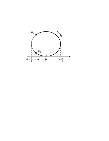
Figure 1. $b>2$

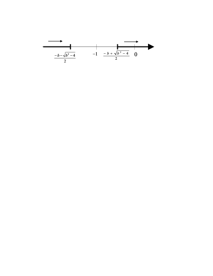
Figure 2. $\gamma$ interval

we can see that $h$ traces the highlighted part of the circle on the figure 1 as $\gamma$ moves from $-\infty$ towards $+\infty$. We also notice that the removed point $(\theta,0)$ corresponds to the value of $\gamma=\pm\infty$ while the points $h_{1}$ and $h_{2}$ correspond to the values $\gamma_{1}=\frac{-b-\sqrt{b^{2}-4}}{2}$ and $\gamma_{2}=\frac{-b+\sqrt{b^{2}-4}}{2}$, respectively (see figure 2).

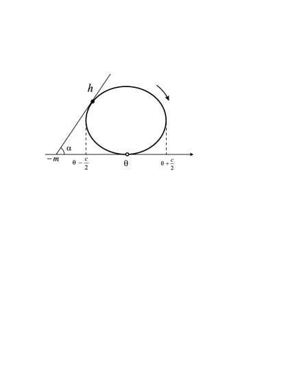
Figure 3. $b<2$

Subcase 2:

$b<2$ For every $\gamma\in(-\infty,+\infty)$ the restored operator $T_{h}$ will be accretive and $\alpha$-sectorial for some $\alpha\in(0,\pi/2)$. As we have mentioned above, the operator $T_{h}$ achieves the largest angle of sectorialilty when $\gamma=-\frac{b}{2}$. In this particular case (5.34) becomes

(5.36) $$h=x+iy,\quad x=\frac{\theta(4-b^{2})-2b^{2}m}{4+b^{2}},\quad y=\frac{4(\theta+m)b}{4+b^{2}}.$$

The value of $h$ from (5.36) is marked on the figure 3.

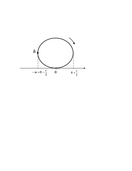
Figure 4. $b=2$

Subcase 3:

$b=2$ The behavior of parameter $h$ in this case is depicted on the figure 4. It shows that in this case the function $V(z)$ can be realized using an extremal accretive $T_{h}$ when $\gamma=-1$. The value of the parameter $h$ according to (5.34) then becomes

(5.37) $$h=x+iy,\quad x=-m,\quad y=\theta+m.$$

Clockwise direction of the circle again corresponds to the change of $\gamma$ from $-\infty$ to $+\infty$ and the marked value of $h$ occurs when $\gamma=-1$.

Now we consider the second case.

Case 2. Here we assume that $\int_{0}^{\infty}\frac{d\sigma(t)}{t}=\infty$. This means that our function $V(z)$ belongs to the class $SL_{0}^{K}(R)$ and $b=\infty$. According to theorem 5.7 and formulas (5.16) and (5.17), the restored operator $T_{h}$ is accretive if and only if

$$\gamma\geq 0,$$

and $\alpha$-sectorial if and only if $\gamma>0$. It directly follows from (5.17) that the exact value of the angle $\alpha$ is then found from

(5.38) $$\tan\alpha=\frac{1}{\gamma}.$$

The latter implies that the restored operator $T_{h}$ is extremal if $\gamma=0$. This means that a function $V(z)\in SL_{0}^{K}(R)$ is realized by a system with an extremal operator $T_{h}$ if and only if

(5.39) $$V(z)=\int\limits_{0}^{\infty}\frac{d\sigma(t)}{t-z}.$$

On the other hand since $\gamma\geq 0$ the function $V(z)$ is a Stieltjes function of the class $S_{0}(R)$. Applying realization theorems from [15] we conclude that $V(z)$ admits realization by an accretive system $\Theta$ of the form (3.1) with ${\mathbb{A}}_{R}$ containing the Krein-von Neumann extension $A_{K}$ as a quasi-kernel. Here $A_{K}$ is defined by (2.8). This yields

(5.40) $$\theta=-m_{\infty}(-0)=-m.$$

As in the beginning of the previous case we derive the formulas for $x$ and $y$, where $h=x+iy$. Using (5.30) and (5.32) leads to

(5.41) $$\begin{cases}\theta=\frac{\mu x-(x^{2}+y^{2})}{\mu-x},&\\ x=\theta+\gamma y.&\end{cases}$$

Solving this system for $x$ and $y$ leads to

(5.42) $$x=\frac{\theta+\mu\gamma^{2}}{1+\gamma^{2}},\quad y=\frac{(\mu-\theta)\gamma}{1+\gamma^{2}}.$$

Combining (5.41) and (5.42) gives

(5.43) $$x=\frac{-m+\mu\gamma^{2}}{1+\gamma^{2}},\quad y=\frac{(m+\mu)\gamma}{1+\gamma^{2}}.$$

To proceed, we first notice that our function $V(z)$ satisfies the conditions of theorem 4.8 of [6]. Indeed, the inequality

$$\mu\geq\frac{({\rm Im\,}h)^{2}}{m_{\infty}(-0)+{\rm Re\,}h}+{\rm Re\,}h,$$

turns into

$$\mu=\frac{y^{2}}{x-m}+x,$$

if you use $\theta=-m$ and the first equation in (5.41). Applying theorem 4.8 of [6] yields

(5.44) $$\int\limits_{0}^{\infty}\frac{d\sigma(t)}{1+t^{2}}=\frac{{\rm Im\,}h}{|\mu-h|^{2}}\left(\sup\limits_{y\in D(A_{K})}\frac{|\mu y(a)-y^{\prime}(a)|}{\left(\int\limits_{a}^{\infty}\left(|y(x)|^{2}+|l(y)|^{2}\right)dx\right)^{\frac{1}{2}}}\right)^{2}.$$

Taking into account that

$$\mu y(a)-y^{\prime}(a)=(\mu+m)y(a)$$

and setting

(5.45) $$c^{1/2}=\sup\limits_{y\in D(A_{K})}\frac{|y(a)|}{\left(\int\limits_{a}^{\infty}\left(|y(x)|^{2}+|l(y)|^{2}\right)dx\right)^{\frac{1}{2}}},$$

we obtain

(5.46) $$\frac{{\rm Im\,}h}{|\mu-h|^{2}}(\mu+m)^{2}\,c=\int\limits_{0}^{\infty}\frac{d\sigma(t)}{1+t^{2}}.$$

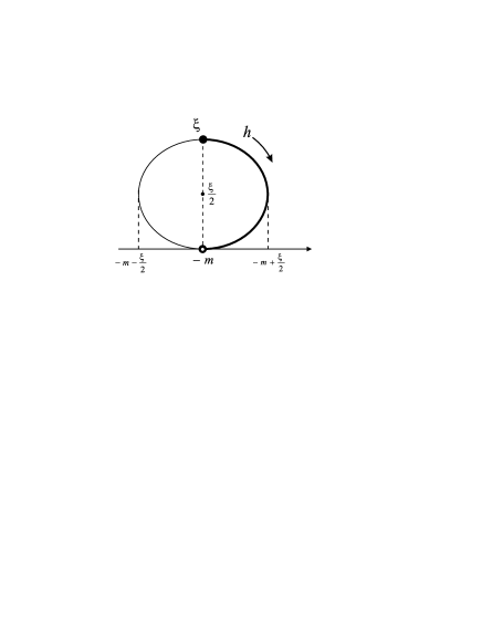
Figure 5. $b=\infty$

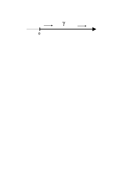
Figure 6. $\gamma\geq 0$

Considering that ${\rm Im\,}h=y$ and combining (5.46) with (5.43) we use straightforward calculations to get

$$\mu=-m+\left(\frac{1}{\gamma\,c}\right)\,\int\limits_{0}^{\infty}\frac{d\sigma(t)}{1+t^{2}}.$$

Let

(5.47) $$\xi=\frac{1}{c}\int_{0}^{\infty}\frac{d\sigma(t)}{1+t^{2}}.$$

Then the last equation becomes

(5.48) $$\mu=-m+\frac{\xi}{\gamma}.$$

Applying (5.48) on (5.43) yields

(5.49) $$x=-m+\frac{\gamma\,\xi}{1+\gamma^{2}},\quad y=\frac{\xi}{1+\gamma^{2}},\qquad\gamma\geq 0.$$

Following the previous case approach we transform (5.49) into

(5.50) $$(x+m)^{2}+\left(y-\frac{\xi}{2}\right)^{2}=\frac{\xi^{2}}{4}.$$

The connection between the parameters $\gamma$ and $h$ in the accretive restored operator $T_{h}$ is depicted in figures 5 and 6. As we can see $h$ traces the highlighted part of the circle clockwise on the figure 5 as $\gamma$ moves from $0$ towards $+\infty$.

As we mentioned earlier the restored operator $T_{h}$ is extremal if $\gamma=0$. In this case formulas (5.49) become

(5.51) $$x=-m,\quad y=\xi,\qquad\gamma=0,$$

where $\xi$ is defined by (5.47).

6. Realizing systems with Schrödinger operator

Now once we described all the possible outcomes for the restored accretive operator $T_{h}$, we can concentrate on the main operator ${\mathbb{A}}$ of the system (5.13). We recall that ${\mathbb{A}}$ is defined by formulas (2.6) and beside the parameter $h$ above contains also parameter $\mu$. We will obtain the behavior of $\mu$ in terms of the components of our function $V(z)$ the same way we treated the parameter $h$. As before we consider two major cases dividing them into subcases when necessary.

Case 1. Assume that $b=\int_{0}^{\infty}\frac{d\sigma(t)}{t}<\infty$. In this case our function $V(z)$ belongs to the class $SL^{K}_{01}(R)$. First we will obtain the representation of $\mu$ in terms of $x$ and $y$, where $h=x+iy$. We recall that

$$\mu=\frac{h-a\bar{h}}{1-a},$$

where $a$ is defined by (5.31). By direct computations we derive that

$$a=\frac{1-\gamma^{2}}{1+\gamma^{2}}-\frac{2\gamma}{1+\gamma^{2}}i,\quad 1-a=\frac{2\gamma^{2}}{1+\gamma^{2}}+\frac{2\gamma}{1+\gamma^{2}}i,$$

and

$$h-a\bar{h}=\left(\frac{2\gamma^{2}}{1+\gamma^{2}}x+\frac{2\gamma}{1+\gamma^{2}}y\right)+\left(\frac{2}{1+\gamma^{2}}y+\frac{2\gamma}{1+\gamma^{2}}x\right)i.$$

Plugging the last two equations into the formula for $\mu$ above and simplifying we obtain

(6.1) $$\mu=x+\frac{1}{\gamma}\,y.$$

We recall that during the present case $x$ and $y$ parts of $h$ are described by the formulas (5.34).

Once again we elaborate in three subcases.

Subcase 1:

$b>2$ As we have shown this above, the formulas (5.34) can be transformed into equation of the circle (5.35). In this case the parameter $\gamma$ belongs to the interval in (5.26), the accretive operator $T_{h}$ corresponds to the values of $h$ shown in the bold part of the circle on the figure 1 as $\gamma$ moves from $-\infty$ towards $+\infty$.

Substituting the expressions for $x$ and $y$ from (5.34) into (6.1) and simplifying we get

(6.2) $$\mu=\theta+\frac{(\theta+m)b}{\gamma}.$$

The connection between values of $\gamma$ and $\mu$ is depicted on the figure 7.

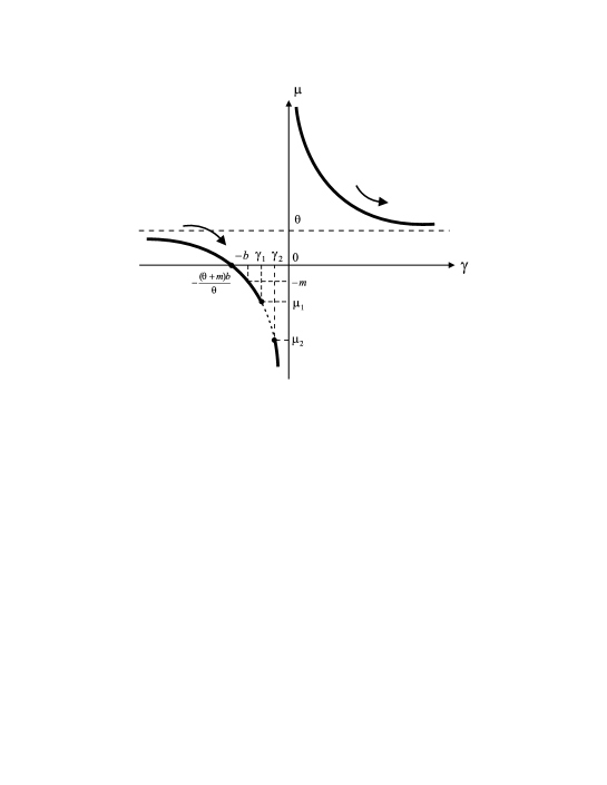
Figure 7. $b>2$

We note that $\mu=0$ when $\gamma=-\frac{(\theta+m)b}{\theta}$. Also, the endpoints

$$\gamma_{1}=\frac{-b-\sqrt{b^{2}-4}}{2}\quad\textrm{ and }\quad\gamma_{2}=\frac{-b+\sqrt{b^{2}-4}}{2}$$

of $\gamma$-interval (5.26) are responsible for the $\mu$-values

$$\mu_{1}=\theta+\frac{(\theta+m)b}{\gamma_{1}}\quad\textrm{ and }\quad\mu_{2}=\theta+\frac{(\theta+m)b}{\gamma_{2}}.$$

The values of $\mu$ that are acceptable parameters of operator ${\mathbb{A}}$ of the restored system make the bold part of the hyperbola on the figure 7. It follows from theorem 4.2 that the operator ${\mathbb{A}}$ of the form (2.6) is accretive if and only if $\gamma\geq 0$ and thus $\mu$ sweeps the right branch on the hyperbola. We note that figure 7 shows the case when $-m<0$, $\theta>0$, and $\theta>-m$. Other possible cases, such as ($-m<0$, $\theta<0$, $\theta>-m$), ($-m<0$, $\theta=0$), and ($m=0$, $\theta>0$) require corresponding adjustments to the graph shown in the picture 7.

Subcase 2:

$b<2$ For every $\gamma\in(-\infty,+\infty)$ the restored operator $T_{h}$ will be accretive and $\alpha$-sectorial for some $\alpha\in(0,\pi/2)$. As we have mentioned above, the operator $T_{h}$ achieves the largest angle of sectorialilty when $\gamma=-\frac{b}{2}$. In this particular case (5.34) becomes

$$h=x+iy,\quad x=\frac{\theta(4-b^{2})-2b^{2}m}{4+b^{2}},\quad y=\frac{4(\theta+m)b}{4+b^{2}}.$$

Substituting $\gamma=b/2$ into (6.1) we obtain

(6.3) $$\mu=-(\theta+2m).$$

This value of $\mu$ from (6.3) is marked on the figure 8. The corresponding operator ${\mathbb{A}}$ of the realizing system is based on these values of parameters $h$ and $\mu$.

Figure 8. $b<2$ and $b=2$

Subcase 3:

$b=2$ The behavior of parameter $\mu$ in this case is also shown on the figure 8. It was shown above that in this case the function $V(z)$ can be realized using an extremal accretive $T_{h}$ when $\gamma=-1$. The values of the parameters $h$ and $\mu$ then become

$$h=x+iy,\quad x=-m,\quad y=\theta+m,\quad\mu=-(\theta+2m).$$

The value of $\mu$ above is marked on the left branch of the hyperbola and occurs when $\gamma=-1=-b/2$.

Case 2. Again we assume that $\int_{0}^{\infty}\frac{d\sigma(t)}{t}=\infty$. Hence $V(z)\in SL_{0}^{K}(R)$ and $b=\infty$. As we mentioned above the restored operator $T_{h}$ is accretive if and only if $\gamma\geq 0$ and $\alpha$-sectorial if and only if $\gamma>0$. It is extremal if $\gamma=0$. The values of $x$, $y$, and $\mu$ were already calculated and are given in (5.49) and (5.48), respectively. That is

$$x=-m+\frac{\gamma\,\xi}{1+\gamma^{2}},\quad y=\frac{\xi}{1+\gamma^{2}},\quad\mu=-m+\frac{\xi}{\gamma},\qquad\gamma\geq 0.$$

where $\xi$ is defined in (5.47). Figure 9 gives graphical representation of this case. Only the right bold branch of hyperbola shows the values of $\mu$ in the case $b=\infty$. If $m=0$ then

$$\mu=\frac{\xi}{\gamma}$$

and the graph should be adjusted accordingly.

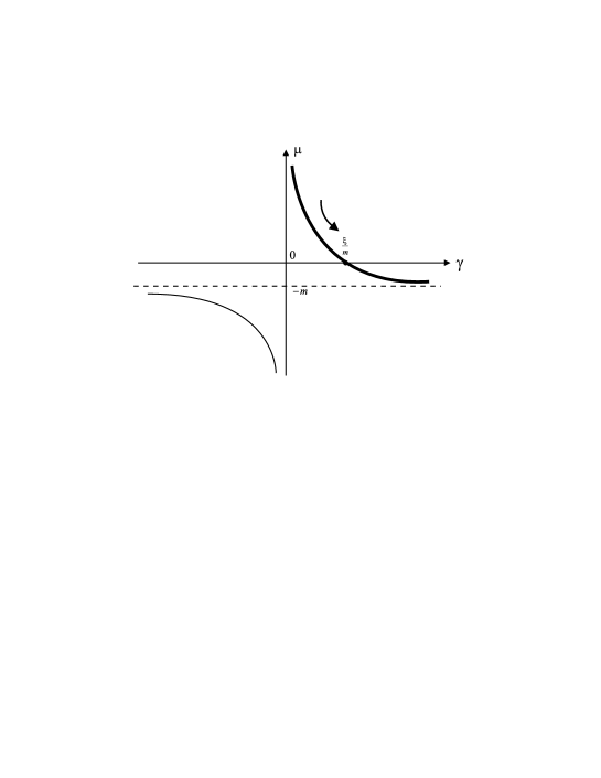
Figure 9. $b=\infty$

In the case when $\gamma=0$ and $T_{h}$ is extremal we have

(6.4) $$x=-m,\quad y=\xi,\quad\mu=\infty,\quad h=-m+i\xi,$$

and according to (2.6) we have

(6.5) $${\mathbb{A}}y=-y^{\prime\prime}+q(x)y+[(-m+i\xi)y(a)-y^{\prime}(a)]\delta(x-a),$$

that is the main operator of the realizing system.

Example

We conclude this paper with simple illustration. Consider a function

(6.6) $$V(z)=\frac{i}{\sqrt{z}}.$$

A direct check confirms that $V(z)$ is a Stieltjes function. It was shown in [23] (see pp. 140-142) that the inversion formula

(6.7) $$\sigma(\lambda)=C+\lim_{y\to 0}\frac{1}{\pi}\int_{0}^{\lambda}{\rm Im\,}\left(\frac{i}{\sqrt{}x+iy}\right)\,dx$$

describes the distribution function for a self-adjoint operator

$$\left\{\begin{array}[]{l}\tilde{B}_{0}y=-y^{\prime\prime}\\ y^{\prime}(0)=0.\\ \end{array}\right.$$

The corresponding to $\tilde{B}_{0}$ symmetric operator is

(6.8) $$\left\{\begin{array}[]{l}B_{0}y=-y^{\prime\prime}\\ y(0)=y^{\prime}(0)=0.\\ \end{array}\right.$$

It was also shown in [23] that $\sigma(\lambda)=0$ for $\lambda\leq 0$ and

(6.9) $$\sigma^{\prime}(\lambda)=\frac{1}{\pi\sqrt{\lambda}}\textrm{\ \ for\ \ }\lambda>0.$$

By direct calculations one can confirm that

$$V(z)=\int_{0}^{\infty}\frac{d\sigma(t)}{t-z}=\frac{i}{\sqrt{z}},$$

and that

$$\int_{0}^{\infty}\frac{d\sigma(t)}{t}=\int_{0}^{\infty}\frac{dt}{\pi t^{3/2}}=\infty.$$

It is also clear that the constant term in the integral representation (4.1) is zero, i.e. $\gamma=0$.

Let us assume that $\sigma(t)$ satisfies our definition of spectral distribution function of the pair $B_{0}$, $\tilde{B}_{0}$ given in the section 5. Operating under this assumption, we proceed to restore parameters $h$ and $\mu$ and apply formulas (5.49) for the values $\gamma=0$ and $m=-\theta=0$. This yields $x=0$. To obtain $y$ we first find the value of

$$\int_{0}^{\infty}\frac{d\sigma(t)}{1+t^{2}}=\frac{1}{\sqrt{2}},$$

and then use formula (5.45) to get the value of $c$. This yields $c=1/\sqrt{2}$. Consequently,

$$\xi=\frac{1}{c}\int_{0}^{\infty}\frac{d\sigma(t)}{1+t^{2}}=1,$$

and hence $h=yi=i$. From (5.48) we have that $\mu=\infty$ and (6.5) becomes

(6.10) $${\mathbb{A}}\,y=-y^{\prime\prime}+[iy(0)-y^{\prime}(0)]\delta(x).$$

The operator $T_{h}$ in this case is

$$\left\{\begin{array}[]{l}T_{h}y=-y^{\prime\prime}\\ y^{\prime}(0)=iy(0).\\ \end{array}\right.$$

The channel vector $g$ of the form (3.12) then equals

(6.11) $$g=\delta(x),$$

satisfying

$${\rm Im\,}{\mathbb{A}}=\frac{{\mathbb{A}}-{\mathbb{A}}^{*}}{2i}=KK^{*}=(.,g)g,$$

and channel operator $Kc=cg$, ($c\in{\mathbb{C}}$) with

(6.12) $$K^{*}y=(y,g)=y(0).$$

The real part of ${\mathbb{A}}$

$${\rm Re\,}{\mathbb{A}}\,y=-y^{\prime\prime}-y^{\prime}(0)\delta(x)$$

contains the self-adjoint quasi-kernel

$$\left\{\begin{array}[]{l}\widehat{A}y=-y^{\prime\prime}\\ y^{\prime}(0)=0.\\ \end{array}\right.$$

A system of the Livs̆ic type with Schrödinger operator of the form (5.13) that realizes $V(z)$ can now be written as

$$\Theta=\begin{pmatrix}{\mathbb{A}}&K&1\cr{\mathcal{H}}_{+}\subset L_{2}[a,+\infty)\subset{\mathcal{H}}_{-}&&{\mathbb{C}}\cr\end{pmatrix}.$$

where ${\mathbb{A}}$ and $K$ are defined above. Now we can back up our assumption on $\sigma(t)$ to be the spectral distribution function of the pair $B_{0}$, $\tilde{B}_{0}$. Indeed, calculating the function $V_{\Theta}(z)$ for the system $\Theta$ above directly via formula (3.17) with $\mu=\infty$ and comparing the result to $V(z)$ gives the exact value of $h=i$. Using the reasoning of remark 5.6 we confirm that $\sigma(t)$ is the spectral distribution function of the pair $B_{0}$, $\tilde{B}_{0}$.

Remark 6.1.

All the derivations above can be repeated for a Stieltjes like function

$$V(z)=\gamma+\frac{i}{\sqrt{z}},\qquad-\infty<\gamma<+\infty,\;\gamma\neq 0$$

with very minor changes. In this case the restored values for $h$ and $\mu$ are described as follows:

$$h=x+iy,\quad x=\frac{\gamma}{1+\gamma^{2}},\quad y=\frac{1}{1+\gamma^{2}},\quad\mu=\frac{1}{\gamma}.$$

The dynamics of changing $h$ according to changing $\gamma$ is depicted on the figure 5 where the circle has the center at the point $i/2$ and radius of $1/2$. The behavior of $\mu$ is described by a hyperbola $\mu=1/\gamma$ (see figure 9 with $\theta=0$). In the case when $\gamma>0$ our function becomes Stieltjes and the restored system $\Theta$ is accretive. The operators ${\mathbb{A}}$ and $K$ of the restored system are given according to the formulas (2.6) and (3.14), respectively.

References

[1]
N.I. Akhiezer and I.M. Glazman.
Theory of linear operators.Pitman Advanced Publishing Program, 1981.
[2]
D. Alpay, I. Gohberg, M. A. Kaashoek, A. L. Sakhnovich, “Direct
and inverse scattering problem for canonical systems with a strictly
pseudoexponential potential”, Math. Nachr. 215 (2000), 5 31.
[3]
D. Alpay and E.R. Tsekanovskiĭ, “Interpolation theory in
sectorial Stieltjes classes and explicit system solutions”, Lin.
Alg. Appl., 314 (2000), 91–136.
[4]
Yu.M. Arlinskiĭ.
On regular (*)-extensions and characteristic
matrix valued functions of ordinary differential operators.Boundary value problems for differential operators,
Kiev, 3–13, 1980.
[5]
Yu. Arlinskiĭ and E. Tsekanovskiĭ.
Regular (*)-extension of unbounded operators, characteristic operator-functions
and realization problems of transfer functions of linear systems.Preprint, VINITI, Dep.-2867, 72p., 1979.
[6]
Yu.M. Arlinskiĭ and E.R. Tsekanovskiĭ, “Linear systems
with Schrödinger operators and their transfer functions”, Oper.
Theory Adv. Appl., 149, 2004, 47–77.
[7]
D. Arov, H. Dym, “Strongly regular -inner matrix-valued
functions and inverse problems for canonical systems”, Oper. Theory
Adv. Appl., 160, Birkhauser, Basel, (2005), 101–160.
[8]
D. Arov, H. Dym, “Direct and inverse problems for differential
systems connected with Dirac systems and related factorization
problems”, Indiana Univ. Math. J. 54 (2005), no. 6, 1769–1815.
[9]
J.A. Ball and O.J. Staffans, “Conservative state-space
realizations of dissipative system behaviors”, Integr. Equ. Oper.
Theory (Online), Birkhäuser, 2005, DOI
10.1007/s00020-003-1356-3.
[10] H. Bart, I. Gohberg, and M. A. Kaashoek, Minimal
Factorizations of Matrix and Operator Functions, Operator Theory:
Advances and Applications, Vol. 1, Birkhäuser, Basel, 1979.
[11]
S.V. Belyi and E.R. Tsekanovskiĭ, “Realization theorems for
operator-valued -functions”, Oper. Theory Adv. Appl., 98 (1997),
55–91.
[12]
S.V. Belyi and E.R. Tsekanovskiĭ, “On classes of realizable
operator-valued -functions”, Oper. Theory Adv. Appl., 115
(2000), 85–112.
[13]
M.S. Brodskiĭ, Triangular and Jordan representations
of linear operators, Moscow, Nauka, 1969 (Russian).
[15]
I. Dovzhenko and E.R. Tsekanovskiĭ, “Classes of Stieltjes
operator-functions and their conservative realizations”, Dokl.
Akad. Nauk SSSR, 311 no. 1 (1990), 18–22.
[16]
F. Gesztesy and E.R. Tsekanovskiĭ, “On matrix-valued Herglotz
functions”, Math. Nachr., 218 (2000), 61–138.
[17] F. Gesztesy, N.J. Kalton, K.A. Makarov, E. Tsekanovskiĭ,
“Some Applications of Operator-Valued Herglotz Functions”,
Operator Theory: Advances and Applications, 123, Birkhäuser,
Basel, (2001), 271–321.
[18] S. Khrushchev, “Spectral Singularities of dissipative
Schrödinger operator with rapidly decreasing potential”, Indiana
Univ. Math. J., 33 no. 4, (1984), 613–638.
[19] I. S. Kac and M. G. Krein, -functions–analytic functions mapping the upper halfplane into
itself, Amer. Math. Soc. Transl. (2) 103, 1-18 (1974).
[20]
Kato T.: Perturbation Theory for Linear Operators, Springer-Verlag,
1966
[21] B. M. Levitan, Inverse
Sturm-Liouville Problems, VNU Science Press, Utrecht, 1987.
[22]
M.S. Livšic, Operators, oscillations, waves, Moscow,
Nauka, 1966 (Russian).
[23] M. A. Naimark, Linear Differential
Operators II, F. Ungar Publ., New York, 1968.
[24]
O.J. Staffans, “Passive and conservative continuous time
impedance and scattering systems, Part I: Well posed systems”,
Math. Control Signals Systems, 15, (2002), 291–315.
[25]
E.R. Tsekanovskiĭ, “Accretive extensions and problems on
Stieltjes operator-valued functions realizations”, Oper. Theory
Adv. Appl., 59 (1992), 328–347.
[26] E.R. Tsekanovskiĭ. “Characteristic function and sectorial boundary value problems”,
Investigation on geometry and math. analysis, Novosibirsk, 7,
(1987), 180–194.
[27]
E.R. Tsekanovskiĭ and Yu.L. Shmul’yan, “The theory of
bi-extensions of operators on rigged Hilbert spaces. Unbounded
operator colligations and characteristic functions”, Russ. Math.
Surv., 32 (1977), 73–131.
[28]
V.A. Yurko, Inverse problems for differential operators,
Saratv State University Publ., Saratov, 1989 (in Russian).