Adaptively Biased Molecular Dynamics for Free Energy Calculations

Abstract

We present an Adaptively Biased Molecular Dynamics (ABMD) method for the computation of the free energy surface of a reaction coordinate using non-equilibrium dynamics. The ABMD method belongs to the general category of umbrella sampling methods with an evolving biasing potential, and is inspired by the metadynamics method. The ABMD method has several useful features, including a small number of control parameters, and an $O(t)$ numerical cost with molecular dynamics time $t$. The ABMD method naturally allows for extensions based on multiple walkers and replica exchange, where different replicas can have different temperatures and/or collective variables. This is beneficial not only in terms of the speed and accuracy of a calculation, but also in terms of the amount of useful information that may be obtained from a given simulation. The workings of the ABMD method are illustrated via a study of the folding of the Ace-GGPGGG-Nme peptide in a gaseous and solvated environment.

I Introduction

When investigating the equilibrium properties of a complex polyatomic system, it is customary to identify a suitable reaction coordinate $\sigma(\mathbf{r}_{1},\dots,\mathbf{r}_{N}):\mathbb{R}^{3N}\mapsto\mathbb{Q}$ that maps atomic positions $\mathbf{r}_{1},\dots,\mathbf{r}_{N}$ onto the points of some manifold $\mathbb{Q}$, and then to study its equilibrium probability density:

$$p(\xi)=\big{<}\delta\left[\xi-\sigma(\mathbf{r}_{1},\dots,\mathbf{r}_{N})\right]\big{>},\;\xi\in\mathbb{Q}$$

(angular brackets denote an ensemble average). The density $p(\xi)$ provides information about the relative stability of states corresponding to different values of $\xi$ along with useful insights into the transitional kinetics between various stable states. In practice, the Landau free energyFrenkel and Smit (2002)

$$f(\xi)=-k_{B}T\ln p(\xi),$$

is typically preferred over $p(\xi)$, because it tends to be more intuitive. Either $p(\xi)$ or $f(\xi)$ is said to provide a coarse-grained description of the system — in terms of $\xi$ alone — with the rest of the degrees of freedom of the original system integrated out. Quite naturally, the reaction coordinate (often also referred to as collective variable or order parameter) is typically chosen to represent the slowest degrees of freedom of the original system, although this is not formally required.

In the past few years, several methods targeting the computation of $f(\xi)$ using non-equilibrium dynamics have become popular. First methods that introduced a time evolving potential to bias the original potential energy were the the Local Elevation Method (LEM)Huber et al. (1994), by Huber, Torda and van Gunsteren in the MD context and the Wang-Landau approach in MC oneWang and Landau (2001). More recent approaches include the adaptive-force bias methodDarve and Pohorille (2001), and the non-equilibrium metadynamicsLaio and Parrinello (2002); Iannuzzi et al. (2003) method. These methods all estimate the free energy of the reaction coordinate from an “evolving” ensemble of realizationsLelièvre et al. (2007); Bussi et al. (2006a), and use that estimate to bias the system dynamics, so as to flatten the effective free energy surface. Collectively, they can all be considered as umbrella sampling methods, with an evolving potential. In the long time limit, the biasing force is expected to compensate for the free energy gradient, so that the biasing potential eventually reproduces the free energy surface.

In this work, we present an Adaptively Biased Molecular Dynamics (ABMD) method whose implementation is particularly efficient and suited for free energy calculations. The method has an $O(t)$ scaling with molecular dynamics time t and is characterized by only two control parameters. In addition, the method allows for extensions based on multiple walkers and replica exchange for both temperature and/or the collective variables. The ABMD method has been implemented in the AMBER software packageCase et al. (2005), and is to be distributed freely.

Before discussing ABMD, it is helpful to review the salient features of the metadynamics (MTD) method. Essentially, the MTD method is built upon the LEM method by exploiting Car-Parrinello dynamics: the phase space of the system is extended to include additional dynamical degrees of freedom harmonically coupled to the collective variable. These additional degrees of freedom are assumed to have masses associated with them, and evolve in time according to Newton’s laws. The masses are supposed to be large enough, so that the dynamics of these extra-variables is driven by the free energy gradient. Their trajectory is then used to construct a history-dependent biasing potential by means of placing many small Gaussians along the trajectory. When combined with Car-Parrinello ab-initio dynamics, MTD has been successfully used to explore complex reaction pathways involving several energy barriersEnsing et al. (2004); Churakov et al. (2004); Gervasio et al. (2005); Ceccarelli et al. (2004); Iannuzzi and Parrinello (2004); A. Stirling and Parrinello (2004); Asciutto and Sagui (2005); Lee et al. (2006); Ikeda et al. (2005).

While MTD continues to be used successfully, there are several known limitations associated with the initial implementation of the method, which provided the motivation for the development of the ABMD method. First, in order to calculate reliable free energies with a controllable accuracy, long runs are needed, especially for the “corrective” follow-up at equilibriumBabin et al. (2006). This is especially true for biomolecular systems, which typically are characterized by many degrees of freedom and non-negligible entropy contributions to the free energies. Long runs, however, may be precluded by the MTD method, because of its unfavorable scaling with molecular dynamics MD time $t$. While one can readily speed up the original MTD method using such tricks as truncated Gaussians and kd-treesBabin et al. (2006), the bottleneck there is the explicit calculation of the history-dependent potential. Since at every MD step, Gaussians from all previous time steps need to be added, the number of Gaussians grows linearly with $t$. The numerical cost of MTD therefore grows as $O(t^{2})$ which, in some cases, may prove itself to be prohibitively expensive, especially when long runs are needed. Another undesirable feature is that the MTD method (at least in its original implementation) is characterized by a relatively large number of parameters (e.g., the masses and spring constants associated with the collective variable, the characteristics of the Gaussians to be added, multiple control parameters, etc), all of which influence the dynamics in an entangled and non-transparent way. A successful MTD run often requires a careful balancing of these parameters, which is especially nontrivial for multidimensional collective variables. More recent implementations of MTD Laio et al. (2005) have reduced the number of parameters. As will be discussed, the ABMD method is characterized by only two control parameters and scales as $O(t)$ with simulation time.

II The Adaptively Biased Molecular Dynamics Method.

The ABMD method is formulated in terms of the following set of equations:

$$m_{a}\frac{\mathrm{d}^{2}\mathbf{r}_{a}}{\mathrm{d}t^{2}}=\mathbf{F}_{a}-\frac{\partial}{\partial\mathbf{r}_{a}}U\big{[}t|\sigma\left(\mathbf{r}_{1},\dots,\mathbf{r}_{N}\right)\big{]},$$

$$\frac{\partial U(t|\xi)}{\partial t}=\frac{k_{B}T}{\tau_{F}}G\big{[}\xi-\sigma\left(\mathbf{r}_{1},\dots,\mathbf{r}_{N}\right)\big{]},$$

where the first set represents Newton’s equations that govern ordinary MD (temperature and pressure regulation terms are not shown) augmented with the additional force coming from the time-dependent biasing potential $U(t|\xi)$ (with $U(t=0|\xi)=0$), whose time evolution is given by the second equation. In the following, we refer to $\tau_{F}$ as flooding timescale and to $G(\xi)$ as kernel (in analogy to the kernel density estimator widely used in statisticsSilverman (1986)). The kernel is supposed to be positive definite ($G(\xi)>0$) and symmetric ($G(-\xi)=G(\xi)$). It can be perceived as a smoothed Dirac delta function. For large enough $\tau_{F}$ and small enough width of the kernel, the biasing potential $U(t|\xi)$ converges towards $-f(\xi)$ as $t\to\infty$Lelièvre et al. (2007); Bussi et al. (2006a).

Our numerical implementation of the ABMD method involves the following. We stick with $\mathbb{Q}=\mathbb{Q}_{1}\times\dots\times\mathbb{Q}_{D}$ where $\mathbb{Q}_{k}$ is either $[a,b]\in\mathbb{R}^{1}$ or a one-dimensional torus, and use cubic B-splines (or products of thereof for $D>1$) to discretize $U(t|\xi)$ in $\mathbb{Q}$:

$$U(t|\xi)=\sum\limits_{m\in\mathbb{Z}^{D}}U_{m}(t)B(\xi/\Delta\xi-m),$$

$$B(\xi)=\left\{\begin{array}[]{ll}(2-|\xi|)^{3}/6,&1\leq|\xi|<2,\\ \xi^{2}(|\xi|-2)/2+2/3,&0\leq|\xi|<1,\\ 0,&\mathrm{otherwise}.\end{array}\right.$$

We use the biweight kernelSilverman (1986) for $G(\xi)$:

$$G(\xi)=\frac{48}{41}\left\{\begin{array}[]{ll}\left(1-\left.\xi^{2}\right/4\right)^{2},&-2\leq\xi\leq 2\\ 0,&\mathrm{otherwise}\end{array}\right.,$$

and an Euler-like discretization scheme for the time evolution of the biasing potential:

$$U_{m}(t+\Delta t)=U_{m}(t)+\Delta t\frac{k_{B}T}{\tau_{F}}G\big{[}\sigma/\Delta\xi-m\big{]},$$

where $\sigma=\sigma(\mathbf{r}_{1},\dots,\mathbf{r}_{N})$ is at time $t$. Note that this time discretization may be readily improved. This, however, is not really important here, since the goal is not to recover the solution of the ABMD equations per se, but rather to flatten $U(t|\xi)+f(\xi)$ in the $t\to\infty$ limit. Note also, that the numerical cost of evaluation of the time-dependent potential is constant over time, and so ABMD scales trivially as $O(t)$, which is computationally quite favorable. The storage requirements of the ABMD are also quite reasonable, especially if sparse arrays are used for $U_{m}$. In addition, it is characterized by only two control parameters: the flooding timescale $\tau_{F}$ and the kernel width $4\Delta\xi$.

ABMD admits two important extensions. The first is identical in spirit to the multiple walkers metadynamicsLelièvre et al. (2007); Raiteri et al. (2006). It amounts to carrying out several different MD simulations biased by the same $U(t|\xi)$, which evolves via:

$$\frac{\partial U(t|\xi)}{\partial t}=\frac{k_{B}T}{\tau_{F}}\sum\limits_{\alpha}G\big{[}\xi-\sigma\left(\mathbf{r}_{1}^{\alpha},\dots,\mathbf{r}_{N}^{\alpha}\right)\big{]}\;,$$

where $\alpha$ labels different MD trajectories. A second extension is to gather several different MD trajectories, each bearing its own biasing potential and, if desired, its own distinct collective variable, into a generalized ensemble for “replica exchange” with modified “exchange” rulesSugita et al. (2000); Bussi et al. (2006b); Piana and Laio (2007). Both extensions are advantageous and lead to a more uniform flattening of $U(t|\xi)+f(\xi)$ in $\mathbb{Q}$. This enhanced convergence to $f(\xi)$ is due to the improved sampling of the “evolving” canonical distribution.

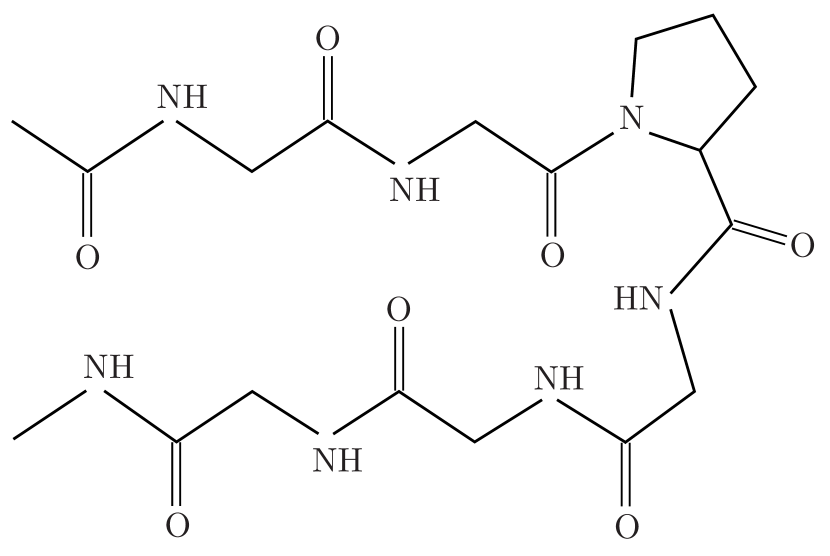
Figure 1: The Ace-GGPGGG-Nme peptide in a $\beta$-hairpin conformation (sketch).

We have implemented the ABMD method in the AMBER packageCase et al. (2005), with support for both replica exchange and multiple-walkers. In pure “parallel tempering” replica exchange (same collective variable in all replicas), $N_{r}$ replicas are simulated at different temperatures $T_{n}$, $n=1,\dots,N_{r}$. Each replica has its own biasing potential $U^{n}(t|\xi)$, $n=1,\dots,N_{r}$, that evolves according to its dynamical equation. Exchanges between neighboring replicas are attempted at a prescribed rate, with an exchange probability given bySugita et al. (2000):

$$w(m|n)=\left\{\begin{array}[]{ll}1,&\Delta\leq 0,\\ \exp(-\Delta),&\Delta>0,\end{array}\right.$$ (1)

$$\Delta = \left(\frac{1}{k_{B}T_{n}}-\frac{1}{k_{B}T_{m}}\right)\Big{(}E_{p}^{m}-E_{p}^{n}\Big{)}$$

$$+ \frac{1}{k_{B}T_{m}}\Big{[}U^{m}(\xi^{n})-U^{m}(\xi^{m})\Big{]}$$

$$- \frac{1}{k_{B}T_{n}}\Big{[}U^{n}(\xi^{n})-U^{n}(\xi^{m})\Big{]},$$

where $E_{p}$ denotes the atomic potential energy. The biasing potentials are temperature-bound and converge in the $t\to\infty$ limit to the free energies at their respective temperatures.

We have also implemented a more general replica exchange scheme, where different replicas can have different collective variables and/or temperatures, and can experience either an evolving or a static biasing potential (the latter obviously includes the case of $U^{n}(t|\xi)=0$). Exchanges between random pairs of replicas are then tried at a prescribed rate. This method is simply a generalization Piana and Laio (2007) of the “Hamiltonian replica exchange” method described in Ref.Sugita et al., 2000, and reduces to it when all biasing potentials are static. The big advantage here is that, by using replicas with different collective variables, it is possible to obtain several one- or two-dimensional projections of the free energy surface for the corresponding variables. This is very useful because it not only increases the amount of information that can be gathered from a given simulation, but it also allows for previously obtained information for a collective variable to be used to compute the free energy associated with different variables. For instance, suppose that in the course of a simulation it becomes apparent that one wishes to address additional questions involving different collective variables. Instead of starting from “scratch”, one can re-use the already obtained biasing potentials and thereby greatly accelerate the free energy calculation for the new variables. It is also worth noting that for replicas running at the same temperature, the exchange probability does not depend on the atomic potential energies (Eqs. (1)-(II) above). This implies that the number of replicas needed to maintain acceptable exchange rates can be made independent of the solvent degrees of freedom, provided that one is interested in the properties of the solute only (so that the collective variables do not depend explicitly on the atomic coordinates of the solvent) and that the structure is adequately solvated. This can be exploited to sample a solute with a minimum amount of solvent, and to accelerate the averaging over the solvent degrees of freedom. These last two applications of the general replica exchange method are illustrated in the next section.

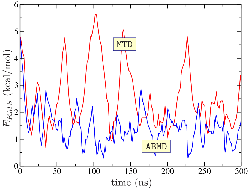
Figure 2: RMS error of the free energy over $3.3\text{\AA}<R_{g}<6.3\text{\AA}$ at $T=300K$ for the ABMD (blue) and reference MTD (red) simulations.

III Case study: a short peptide.

To illustrate the method, we have simulated the hydrophobic Ace-GGPGGG-Nme peptide (sketched in Fig.1) in the gas phase and in a solvated environment, using cyclohexane as the explicit solvent. The free energy of this peptide at $T=300\,\mathrm{K}$ in gas phase has previously been investigated with the MTD methodBabin et al. (2006), and is characterized by a “double-well” structure (see Fig.8), with the wells corresponding to the peptide in a “globular” (left minimum in the Fig.8) and a $\beta$-hairpin (right minimum in the Fig.8) folded conformation, respectively. While simple enough, the molecule possesses all the typical features of larger peptide systems usually studied with biomolecular simulations. Simulation parameters are as in a previous studyBabin et al. (2006): the atoms are described by the 1999 version of the Cornell et al. force fieldCornell et al. (1995), with no cutoff for the non-bonded interactions. The Berendsen thermostat is chosen with $\tau_{tp}=1\mathrm{fs}$ for temperature control. The MD time step ($\Delta t$) is 1 fs for the parallel tempering simulations, and 2 fs otherwise.

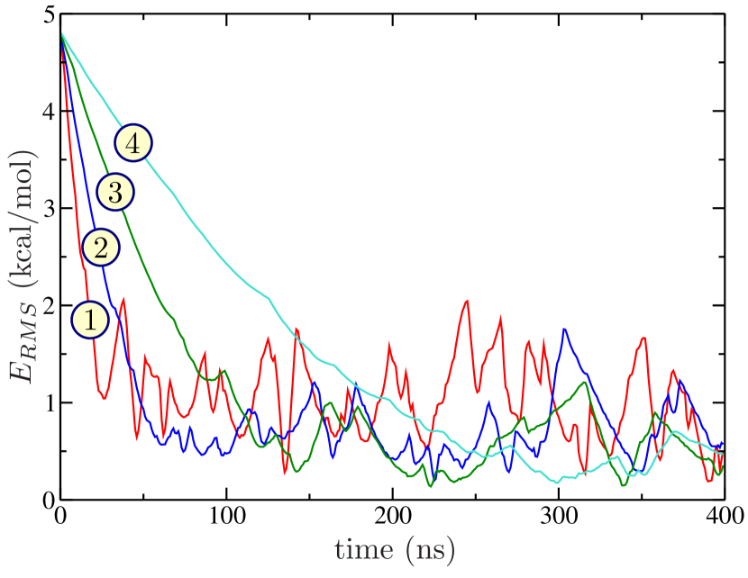
Figure 3: RMS error of the free energy over $3.3\text{\AA}<R_{g}<6.3\text{\AA}$ for ABMD simulations at $T=300K$ with $\tau_{F}=180\;\mathrm{ps}$ (1), $360\;\mathrm{ps}$ (2), $720\;\mathrm{ps}$ (3) and $1440\;\mathrm{ps}$ (4).

The radius of gyration of the heavy atoms was chosen to be the collective variable:

$$R_{g}=\sum_{a}\frac{m_{a}}{m_{\Sigma}}\left(\mathbf{r}_{a}-\mathbf{R}_{\Sigma}\right)^{2}\,.$$ (3)

Here, $\mathbf{R}_{\Sigma}=\sum_{a}\left(m_{a}/m_{\Sigma}\right)\mathbf{r}_{a}$ is the center of mass, with $m_{\Sigma}=\sum_{a}m_{a}$, and the sum runs over all atoms except hydrogen. The initial configuration is the fully unfolded peptide. A reference free energy profile, whose errorBabin et al. (2006) in the region of interest is less than 0.15 kcal/mol, was computed for benchmarking purposes (see Appendix A for details). As a measure of the RMS free energy error, the following construction was used:

$$E_{RMS}=\sqrt{\frac{1}{b-a}\int\limits_{a}^{b}\mathrm{d}\xi\Big{(}f_{1}(\xi)-f_{2}(\xi)-\Delta\Big{)}^{2}},$$

where

$$\Delta=\frac{1}{b-a}\int\limits_{a}^{b}\mathrm{d}\xi\Big{(}f_{1}(\xi)-f_{2}(\xi)\Big{)},$$

accounts for the arbitrary additive constants in the free energies $f_{1,2}(\xi)$. Here $a=3.3$Å and $b=6.3$Å, which correspond to the physical region of interest (see Fig.8).

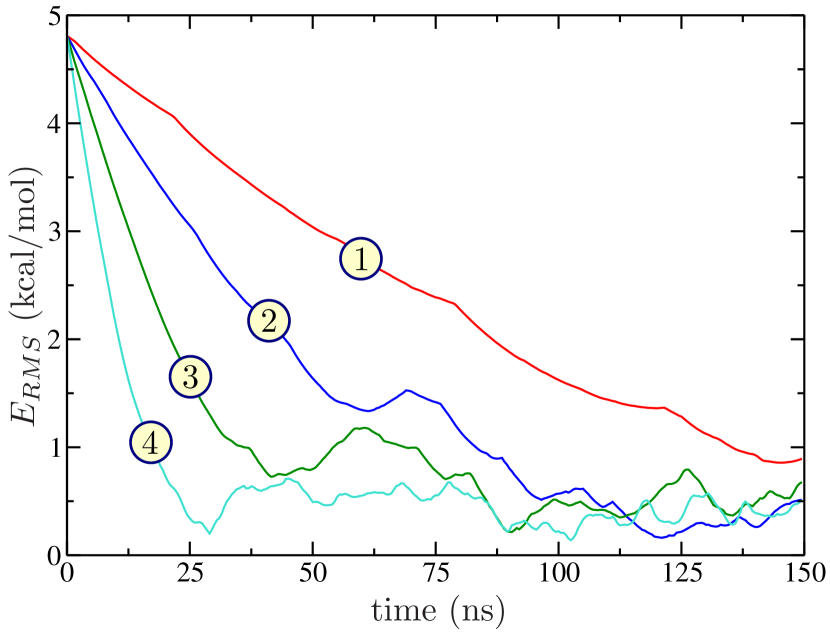
Figure 4: RMS error of the free energy over 3.3Å$<R_{g}<$6.3Å for multiple walkers ABMD simulations with $\tau_{F}=1\,\mathrm{ns}$ using one (1), two (2), four (4) and eight (8) trajectories at $T=300$K.

Figure 2 presents the time dependence of the RMS free energy error for the ABMD and reference MTD runBabin et al. (2006). Both simulations have exactly the same kernel width $4\Delta\xi=0.25\;$Å, and flooding timescale $\tau_{F}=90\;\mathrm{ps}$ that corresponds to the a posteriori hills acceptance rate reported in Ref.Babin et al., 2006. It is evident that the AMBD run is more accurate than the corresponding MTD run. The ABMD method owes its better convergence to the smoother time evolution of the biasing potential and accurate discretization in $\mathbb{Q}$. The amount of memory used by the ABMD simulation to store $U_{m}$ values was only $\approx 200\times 8$ bytes (considering double precision) for roughly $10^{8}$ tiny “hills” that were accumulated by the end of the run. The reference MTD simulation with merely $5\times 10^{3}$ Gaussians required roughly 25 times more memory for the biasing potential (with only the positions of the Gaussians stored explicitly). One can expect, that ABMD will be even more economical when it comes to dealing with multidimensional collective variables, provided that sparse arrays are used for $U_{m}$ with only non-zero elements being stored explicitly.

Although an a priori error estimate for this type of non-equilibrium simulation is really not feasible, it is expected that the error should decrease for increased $\tau_{F}$. This point is illustrated in Fig.3, which shows the error for increasing values of $\tau_{F}$.

In order to decrease the simulation time required for accurate free energy estimates even further, the multiple-walker variation of ABMD proves to be useful. For a moderate number of walkers, the speedup is nearly linear, with an additional increase in accuracy coming from the better sampling of the “evolving” canonical distribution (see Fig.4). Parallel tempering improves both the speed and the accuracy even more. To this end, we first ran ABMD with $\tau_{F}=90\,\mathrm{ps}$ using 2, 4, 6 and 8 replicas at $T=300\,\mathrm{K}$, $331\,\mathrm{K}$, $365\,\mathrm{K}$, $403\,\mathrm{K}$, $445\,\mathrm{K}$, $492\,\mathrm{K}$, $543\,\mathrm{K}$ and $600\,\mathrm{K}$ (during equilibrium MD runs, the peptide configuration jumps between the two minima on a picosecond timescale at $T=600\mathrm{K}$). In all cases, the $E_{RMS}$ was found to be $\sim 1$ kcal/mol, or less as $t\to\infty$ (data not shown). Again, the improvement in accuracy stems from the better sampling of the “evolving” canonical distribution. Then, we ran 8 replicas with smaller values $\tau_{F}$ and were surprised that the accuracy does not degrade, even for $\tau_{F}=11.2\,\mathrm{ps}$ as shown in Fig.5.

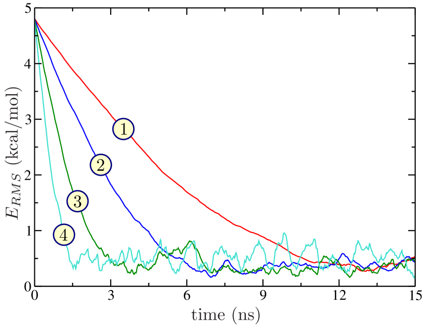
Figure 5: RMS error of the free energy over $3.3\text{\AA}<R_{g}<6.3\text{\AA}$ at $T=300K$ for parallel tempering ABMD simulations using eight replicas running at $T=300\,\mathrm{K}$, $331\,\mathrm{K}$, $365\,\mathrm{K}$, $403\,\mathrm{K}$, $445\,\mathrm{K}$, $492\,\mathrm{K}$, $543\,\mathrm{K}$ and $600\,\mathrm{K}$ with $\tau_{F}=90\,\mathrm{ps}$ (1), $45\,\mathrm{ps}$ (2), $22.5\,\mathrm{ps}$ (3) and $11.25\,\mathrm{ps}$ (4).

Finally, we turn to aspects related to the general replica exchange method and illustrate its potential. As already noted, by using replicas with different collective variables and swapping these at prescribed rates, it is possible to obtain projections of the free energy surface for the corresponding variables. It is also possible to use previously obtained information with respect to one collective variable to compute the free energy associated with a different variable. For example, suppose that instead of the one-dimensional free energy profile as as a function of $R_{g}$ already discussed, one realizes that what is actually needed is a two-dimensional profile that includes information with respect to the number of O-H bonds along the backbone. The two-dimensional free energy map is computationally quite expensive, but the calculation can be greatly accelerated with the help of the general replica exchange method. We therefore simulated $8+1=9$ replicas. The eight replicas were run at the previously stated temperatures, with each replica biased by a static (not evolving) biasing potential corresponding to the negated free energy associated with the radius of gyration $R_{g}$ at the corresponding temperature, as shown in Fig.8. The additional ninth replica was run at $T=300\,\mathrm{K}$ with ABMD flooding in the two collective variables, i.e., $R_{g}$ and the number of O-H bonds along the backbone as given by

$$N_{\mathrm{OH}}=\sum\limits_{\mathrm{O},\mathrm{H}}\frac{1-\big{(}\left.r_{\mathrm{OH}}\right/r_{0}\big{)}^{6\hphantom{1}}}{1-\big{(}\left.r_{\mathrm{OH}}\right/r_{0}\big{)}^{12}}\,,$$

where $r_{\mathrm{OH}}$ is the distance between a pair of hydrogen and oxygen atoms and $r_{0}=2.5\text{\AA}$. The sum runs over the unique O-H pairs (i.e., each O-H pair is counted only once), with O and H separated by one or more amino-bases along the backbone (27 pairs in total). In other words, we “re-use” the previously computed free energies for $R_{g}$ to get the free energy in the two-dimensional space $(R_{g},N_{\mathrm{OH}})$: the eight first replicas serve as a “sampling enhancement device” for the ninth replica. The calculation is carried out in two stages: a “coarse” stage ($15\,\mathrm{ns}$ with $\tau_{F}=10\,\mathrm{ps}$ and $4\Delta R_{g}=0.25\text{\AA}$, $4\Delta N_{\mathrm{OH}}=0.5$) followed by a “fine” stage ($50\,\mathrm{ns}$ with $\tau_{F}=100\,\mathrm{ps}$ and $4\Delta R_{g}=0.1\text{\AA}$, $4\Delta N_{\mathrm{OH}}=0.25$). In both runs exchanges between four randomly chosen pairs of replicas were attempted every $100\,\mathrm{fs}$. The final free energy map is shown in Fig.6. It is clear that this two-dimensional free energy landscape conveys additional information not contained in the one-dimensional free energy plots already discussed. In particular, it allows for a better characterization of the “globular” states of the Ace-GGPGGG-Nme : specifically, it is apparent from the Fig.6 that there are at least two such states with different values of $N_{\mathrm{OH}}$ (both correspond to the left minimum in Fig.8). Of course, one could have re-used the information in the one-dimensional $R_{g}$ profiles to include other collective variables, in addition to $N_{\mathrm{OH}}$.

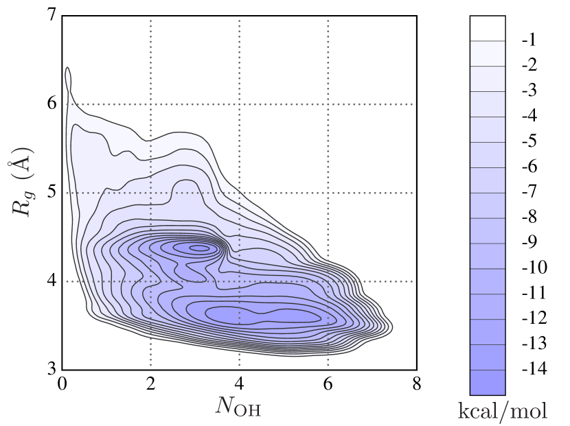
Figure 6: Free energy map for Ace-GGPGGG-Nme peptide in the gas phase as a function of the collective variables $R_{g}$ and $N_{\mathrm{OH}}$. (see Ref.Preusser, 1989 for details regarding the algorithm used to make this plot).

The general replica exchange ABMD may also be advantageous for explicit solvent simulations, which are often notoriously lengthy. Specifically, if one is interested in the solute and the collective variables do not depend on the solvent degrees of freedom, then the number of replicas required to maintain an adequate exchange rate depends only very weakly on the amount of solvent (which must of course be sufficient as to adequately solvate the structure), provided that all the replicas are simulated at the same temperature. This is because the exchange probability does not explicitly depend on the potential energy difference when the temperature of the replicas is the same. While not every choice of collective variables for different replicas will lead to decent exchange rates, one can nevertheless take advantage of this property and use general replica exchange to enhance the sampling in a solvated environment.

In order to demonstrate the method in this regime, we simulated the Ace-GGPGGG-Nme peptide at $T=300\,\mathrm{K}$ solvated by 171 cyclohexane ($\mathrm{C}_{6}\mathrm{H}_{12}$) molecules (the total number of atoms was 3139) under periodic boundary conditions using the GeneralWang et al. (2004) AMBER Force-Field (GAFF) for the solvent. We used a truncated octahedron cell of fixed size (constant volume) that corresponds to the equilibrium density at $T=300\,\mathrm{K}$ (the equilibrium density value was obtained from a $10\,\mathrm{ns}$ simulation under constant pressure at $T=300\,\mathrm{K}$). The Particle-Mesh Ewald (PMEDarden et al. (1993)) method was used for the electrostatic forces, with a $36\times 36\times 36$ FFT grid and an $8\,\text{\AA}$ cutoff for the direct sum (same cutoff was used for van der Waals interactions). First, we ran 10 replicas in the “flooding” mode (i.e., under evolving biasing potentials) using as collective variables the distances $r_{\mathrm{CC}}$ between the backbone carbons separated by at least 2 amino-acids (there are 10 such distances for Ace-GGPGGG-Nme ). We ran for $5\,\mathrm{ns}$ with $\tau_{F}=30\,\mathrm{ps}$ and $4\Delta r_{\mathrm{CC}}=1\text{\AA}$, and then for another $5\,\mathrm{ns}$ with $\tau_{F}=150\,\mathrm{ps}$ and $4\Delta r_{\mathrm{CC}}=0.5\text{\AA}$, attempting exchanges between five randomly selected pairs every $0.5\,\mathrm{ps}$. As expected, at the start of the simulation, the exchange rate was nearly 100% decreasing later as the biasing potentials were built up. By the end of the simulation, when all possible values of the distances had been covered, the exchange rate was very disparate between different pairs of replicas. However, for every replica there was at least one other replica such that the exchange rate between them was reasonable (i.e., the whole simulation did not degenerate into ten different non-interacting trajectories). We then set $\tau_{F}=\infty$ in these 10 replicas, and added an eleventh replica whose collective variable was chosen as the radius of gyration of the heavy atoms. In other words, as before, we use the ten replicas as a “sampling enhancement device” for the last one. We then ran a two-stage flooding scheme: a $5\,\mathrm{ns}$ coarser stage, with $\tau_{F}=25\,\mathrm{ps}$ and $4\Delta R_{g}=0.25\text{\AA}$; followed by a $10\,\mathrm{ns}$ finer stage, with $\tau_{F}=180\,\mathrm{ps}$ and $4\Delta R_{g}=0.2\text{\AA}$. As before, the exchange attempts between 5 randomly selected pairs of replicas were performed every $0.5\,\mathrm{ps}$. The “raw” ABMD-computed free energy associated with $R_{g}$ after that stage is shown in Fig.7. In a next step, we ran 64 biased simulations (each comprising of 11 replicas) for $7\,\mathrm{ns}$ (first $2\,\mathrm{ns}$ for equilibration followed by $5\,\mathrm{ns}$ of “production” runs) starting from different initial configurations. We set $\tau_{F}=\infty$ in all replicas (static biasing potentials) and recorded the values of $R_{g}$ in the eleventh replica every 10 picoseconds. We then used the log-spline algorithm of StoneStone et al. (1997) at. al. to estimate the (biased) log-density of the $R_{g}$ values at equilibrium. This led us to the final shape of the free energy curve shown in Fig.7. Compared to the gas phase, the folded $\beta$-turn in the cyclohexane solvated peptide is clearly favored over the globular structure.

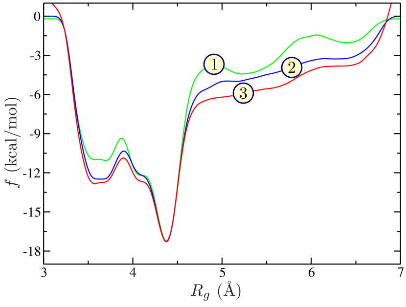
Figure 7: Free energy for Ace-GGPGGG-Nme peptide solvated in cyclohexane at $T=300\,\mathrm{K}$ as obtained via: coarse (non-equilibrium) replica-exchange ABMD (1); finer (non-equilibrium) replica-exchange ABMD (2); including the correction coming from equilibrium biased replica exchange (3).

IV Conclusions and outlook.

In summary, we have presented an ABMD method that computes the free energy surface of a reaction coordinate using non-equilibrium dynamics. The method belongs to the general category of umbrella sampling methods with an evolving potential, and is characterized by only two control parameters (the flooding timescale and the kernel width) and a favorable $O(t)$ scaling with molecular dynamics time t. This scaling can be very important for large-scale classical MD biomolecular simulations when long simulation times are required (see, for example Ref.Shirts et al., 2003, and references therein).

ABMD has also been extended to support multiple walkers and replica exchange. Both variations improve speed and accuracy of the method due to the better sampling of the “evolving” canonical distribution. The replica exchange ABMD has been generalized to include different temperatures and/or collective variables, that move under either an evolving or a static biasing potential. Aside from enhancing the sampling, this swapping of replicas has several important practical advantages. Most importantly, it enables one to obtain projections of the free energy surface for any number of collective variables one might wish to investigate. In addition, one can re-use previously obtained results in order to enhance the sampling of new collective variables. It is also possible to exploit the fact that exchange rates at the same temperature are independent of the potential energy to enhance sampling of a solute in a minimum amount of solvent (for collective variables independent of solvent atom coordinates). We have implemented the ABMD method in the AMBER packageCase et al. (2005), and plan to distribute it freely. Here, we have demonstrated the workings of the ABMD method with a study of the folding of the Ace-GGPGGG-Nme peptide, The application of ABMD to more complicated biomolecular systems is reserved for future publications.

Appendix A Reference free energy curve.

Here, we provide simulation details with regards to the reference free energy curve. We first ran short (5 ns, eight walkers with $\tau_{F}=60\mathrm{ps}$ and $4\Delta\xi=0.2$Å) multiple-walkers ABMD at $T=600\,\mathrm{K}$ to reconstruct the global well. This was followed by parallel tempering ABMD runs, using the biasing potential obtained from the multiple-walkers simulation as the zero-time value for the biasing potentials at different temperatures. We used eight replicas at $T=300\,\mathrm{K}$, $331\,\mathrm{K}$, $365\,\mathrm{K}$, $403\,\mathrm{K}$, $445\,\mathrm{K}$, $492\,\mathrm{K}$, $543\,\mathrm{K}$ and $600\,\mathrm{K}$ and attempted exchanges every 100 MD steps ($0.1\,\mathrm{ps}$). The simulation started with $\tau_{F}=60\mathrm{ps}$ and $4\Delta\xi=0.2$Å, and ran for $10^{5}$ exchanges. We then set $\tau_{F}$ to $600\mathrm{ps}$, $4\Delta\xi$ to $0.1$Å and ran for $5\times 10^{5}$ more exchanges. Finally, this was followed up with $1\times 10^{6}$ more exchanges with $\tau_{F}=6\mathrm{ns}$ and $4\Delta\xi=0.1$Å.

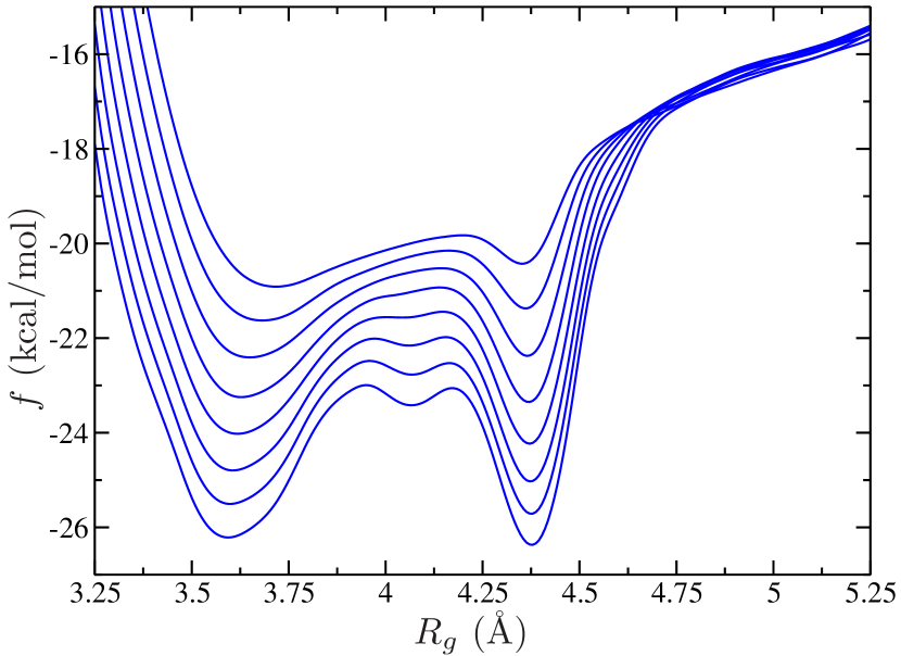
Figure 8: The accurate free energies of Ace-GGPGGG-Nme peptide in gas phase as function of $R_{g}$ at $T=300\,\mathrm{K}$, $331\,\mathrm{K}$, $365\,\mathrm{K}$, $403\,\mathrm{K}$, $445\,\mathrm{K}$, $492\,\mathrm{K}$, $543\,\mathrm{K}$ and $600\,\mathrm{K}$ (from bottom to top).

We then ran a very long ($3\times 10^{7}$ exchanges, $0.1\,\mathrm{ps}$ between exchanges) biased parallel tempering simulation in the spirit of Ref.Babin et al., 2006, in order to get an a posteriori error estimate. From the resulting histogram it follows that the error does not exceed $\approx 0.15\,\mathrm{kcal/mol}$ for 3.3Å$<R_{g}<$6.3Å. The RMS error is probably much smaller, since 0.15 corresponds to the absolute non-uniformity of the histogram, i.e., the maximum error, over 3.3Å$<R_{g}<$6.3Å. The accurate free energy curves as a function of temperature are shown in Fig.8.

References

- Frenkel and Smit (2002) D. Frenkel and B. Smit, Understanding Molecular Simulation, Computational Science Series (Academic Press, 2002).
- Huber et al. (1994) T. Huber, A. E. Torda, and W. F. van Gunsteren, J. Comput. Aided. Mol. Des. 8, 695 (1994).
- Wang and Landau (2001) F. Wang and D. P. Landau, Phys. Rev. Lett. 86, 2050 (2001).
- Darve and Pohorille (2001) E. Darve and A. Pohorille, J. Chem. Phys. 115, 9169 (2001).
- Laio and Parrinello (2002) A. Laio and M. Parrinello, Proc. Natl. Acad. Sci. 99, 12562 (2002).
- Iannuzzi et al. (2003) M. Iannuzzi, A. Laio, and M. Parrinello, Phys. Rev. Lett. 90, 238302 (2003).
- Lelièvre et al. (2007) T. Lelièvre, M. Rousset, and G. Stoltz, J. Chem. Phys. 126, 134111 (2007).
- Bussi et al. (2006a) G. Bussi, A. Laio, and M. Parrinello, Phys. Rev. Lett. 96, 090601 (2006a).
- Case et al. (2005) D. A. Case, T. E. Cheatham, III, T. Darden, H. Gohlke, R. Luo, K. M. Merz, Jr., A. Onufriev, C. Simmerling, B. Wang, and R. Woods, J. Computat. Chem. 26, 1668 (2005).
- Ensing et al. (2004) B. Ensing, A. Laio, F. L. Gervasio, M. Parrinello, and M. L. Klein, J. Am. Chem. Soc. 126, 9492 (2004).
- Churakov et al. (2004) S. V. Churakov, M. Ianuzzi, and M. Parrinello, J. Phys. Chem. B 108, 11567 (2004).
- Gervasio et al. (2005) F. Gervasio, A. Laio, and M. Parrinello, J. Am. Chem. Soc. 124, 2600 (2005).
- Ceccarelli et al. (2004) M. Ceccarelli, C. Danelon, A. Laio, and M. Parrinello, Biophys. J. 87, 58 (2004).
- Iannuzzi and Parrinello (2004) M. Iannuzzi and M. Parrinello, Phys. Rev. Lett. 93, 025901 (2004).
- A. Stirling and Parrinello (2004) A. L. A. Stirling, M. Ianuzzi and M. Parrinello, ChemPhysChem 5, 1558 (2004).
- Asciutto and Sagui (2005) E. Asciutto and C. Sagui, J. Phys. Chem. A 109, 7682 (2005).
- Lee et al. (2006) J. G. Lee, E. Asciutto, V. Babin, C. Sagui, T. A. Darden, and C. Roland, J. Phys. Chem. B 110, 2325 (2006).
- Ikeda et al. (2005) T. Ikeda, M. Hirata, and T. Kimura, J. Chem. Phys. 122, 244507 (2005).
- Babin et al. (2006) V. Babin, C. Roland, T. A. Darden, and C. Sagui, J. Chem. Phys. 125, 204909 (2006).
- Laio et al. (2005) A. Laio, A. Rodriguez-Fortea, F. L. Gervasio, M. Ceccarelli, and M. Parrinello, J. Phys. Chem. B 109, 6714 (2005).
- Silverman (1986) B. W. Silverman, Density Estimation for Statistics and Data Analysis, Monographs on statistics and applied probability (Chapman and Hall, 1986).
- Raiteri et al. (2006) P. Raiteri, A. Laio, F. L. Gervasio, C. Micheletti, and M. Parrinello, J. Phys. Chem. 110, 3533 (2006).
- Sugita et al. (2000) Y. Sugita, A. Kitao, and Y. Okamoto, J. Chem. Phys. 113, 6042 (2000).
- Bussi et al. (2006b) G. Bussi, F. L. Gervasio, A. Laio, and M. Parrinello, J. Am. Chem. Soc. 128, 13435 (2006b).
- Piana and Laio (2007) S. Piana and A. Laio, J. Phys. Chem. B 111, 4553 (2007).
- Cornell et al. (1995) W. D. Cornell, P. Cieplak, C. I. Bayly, I. R. Gould, K. M. Merz, D. M. Ferguson, D. C. Spellmeyer, T. Fox, J. W. Caldwell, and P. A. Kollman, J. Am. Chem. Soc. 117, 5179 (1995).
- Preusser (1989) A. Preusser, ACM Transactions on Mathematical Software 15, 79 (1989).
- Wang et al. (2004) J. Wang, R. Wolf, J. Caldwell, P. Kollman, and D. Case, J. Comp. Chem. 25, 1157 (2004).
- Darden et al. (1993) T. A. Darden, D. M. York, and L. G. Pedersen, J. Chem. Phys. 98, 10089 (1993).
- Stone et al. (1997) C. J. Stone, M. Hansen, C. Kooperberg, and Y. K. Truong, Annals of Statistics 25, 1371 (1997).
- Shirts et al. (2003) M. R. Shirts, J. W. Pitera, W. C. Swope, and V. S. Pande, J. Chem. Phys. 119, 5740 (2003).