Ergodicity of the $\Delta_{3}$ statistic and purity of neutron resonance data

Abstract

The $\Delta_{3}(L)$ statistic characterizes the fluctuations of the number of levels as a function of the length of the spectral interval. It is studied as a possible tool to indicate the regular or chaotic nature of the underlying dynamics, to detect missing levels and the mixing of sequences of levels of different symmetry, particularly in neutron resonance data. The relation between the ensemble average and the average over different fragments of a given realization of spectra is considered. A useful expression for the variance of $\Delta_{3}(L)$ which accounts for finite sample size is discussed. An analysis of neutron resonance data presents the results consistent with a maximum likelihood method applied to the level spacing distribution.

I Introduction

Neutron resonances provided the first context for modeling physical reality with Random Matrix Theory (RMT) Porter (1965); for a brief history of RMT see Guhr et al. (1998). Bohr’s compound nucleus description Bohr (1936) identified the positions of the resonances as eigenvalues of the unknown complicated Hamiltonian governing the compound nucleus. Calculating the energies of these excited states is impossible, even for non-interacting particles the level density is prohibitive just from combinatorics alone; with interactions included, exact calculations even in a reasonably truncated space quickly become impossible. However, robust statistical features of the spectra are calculable. Statistical spectroscopy had already been opened up by Gurevich in 1939 when he investigated the regularities of level spacings in nuclear spectra Gurevich (1939). Wigner took it a step farther in 1951 when he suggested that although the specific energies cannot be calculated, the wave functions are so complicated that the statistical behavior of the energy levels mimics that of the eigenvalues of an ensemble of random matrices whose elements have probability distributions that do not favor any particular basis, i.e. their statistics are invariant under orthogonal transformations (change of basis). The underlying assumption is that the actual Hamiltonian is complicated in any basis excluding some exceptional ones which form a manifold of measure zero. This led, for a time-reversal invariant physical system, to the Gaussian Orthogonal Ensemble (GOE) and, for different global symmetries, to other “canonical” ensembles.

In a sense, canonical Gaussian ensembles describe the extreme degree of universal chaoticity, and the real interest is in understanding when, and to what extent, this limit is realized in actual physical systems. The spectra of quantum systems whose classical counterparts are chaotic are well modeled by the GOE: they have the same spectral fluctuation properties Brody et al. (1981); Stockmann (1999); Bohigas et al. (1984). This leads us to accept RMT as a working definition of quantum chaos: a quantum system is deemed chaotic if its spectra exhibit the same local fluctuation properties as those of the appropriate Gaussian ensemble. This definition frees us from the need to work backwards from classical mechanics.

The correspondence between the GOE and nuclear spectra has been verified many times, over a surprising range of energies. Careful analysis showed that RMT agreed well with the neutron Liou et al. (1972a, b); Jain and Blons (1975); Frankle et al. (1994) and proton Watson III et al. (1981) resonance data for various isotopes. The range of energies at which the nucleus exhibited signatures of chaos was extended all the way to the ground state region in odd-odd nuclei and to two-quasiparticle threshold in even-even nuclei Abul-Magd and Weidenmüller (1985); Shriner Jr. et al. (1991); Raman et al. (1991); Abul-Magd (1996). Furthermore, shell model calculations exhibit many of the fluctuation properties of the GOE Zelevinsky et al. (1996); Horoi et al. (2001); for an account of tests of RMT in nuclei see Mitchell (2001). Ongoing experimental high-precision studies of neutron resonances in heavy nuclei Koehler et al. (2007) require more attention to the details and statistical justification of RMT in its practical applications.

Thus RMT provides us with an arsenal of tools, in the form of certain useful statistics, to analyze neutron resonance data Dyson and Mehta (1963), the largest available body of nuclear spectra. A statistic is a number, $W$, which can be computed from a sequence of levels, and whose mean, $\langle W\rangle$, and variance, ${\rm Var(W)}=\langle W^{2}\rangle-\langle W\rangle^{2}$, are calculable from theory, and which has a small deviation from the theoretical value when the theoretical model is a valid one. In our case, the theoretical model is that the local fluctuations of the energy levels of excited nuclei are described by RMT. To use these statistics, the experimental energies must be rescaled to the uniform level density. This process, called unfolding, removes secular variations of the spectra, leaving just the fluctuations about the mean values, thus allowing spectra from different physical systems to be compared.

Among various statistical measures of spectral fluctuations, the neighboring level spacing distribution $P(s)$, and the Dyson-Mehta $\Delta_{3}(L)$ statistic that quantifies the fluctuations of the number of levels in a given spectral interval, are the most useful in practice. Even their qualitative features allow one to quickly get a first glimpse of the character of underlying dynamics, $-$ regular, chaotic or intermediate. The quantitative analysis provides more detailed characteristics. In order to apply such measures successfully, one needs to know the completeness of a fragment of an empirical spectrum and its purity. Missing levels or contamination by levels of different symmetry classes leads to distortions of the statistics. Apart from that, an important question is that of the ergodicity of those statistical measures. The predictions of RMT refer, as a rule, to the ensemble average of the quantity of interest. Experiment, on the other hand, typically gives the spectral average of the quantity inside an observed subset of the large, formally infinite, spectrum, which is taken as a random representative of an ensemble. The ergodic property means that the same results are valid for different fragments of a given spectrum as well as for the average over the ensemble.

The Dyson-Mehta $\Delta_{3}(L)$ statistic will be the focus of this work. We study fluctuations of this statistic, its ergodic properties and sensitivity to missing levels and impurities. The point of contact with experimental data will be neutron resonance data. There are many other systems that lend themselves to an RMT analysis. The sizes of typical data sets vary from system to system. The spectrum of electromechanical vibrations in a quartz block Guhr et al. (1998), for example, can have many hundreds of levels, as can data from superconducting microwave cavities. Many of the calculations in this paper have $N$ in the hundreds. The main results are still applicable to neutron resonance data, even though the majority of experimental data have less than 100 levels. We provide an error estimate on the calculation of the fraction of missed levels for data sets with $N=100$.

In Sec. II we define the $\Delta_{3}(L)$ and discuss its ensemble average. In Sec. III we discuss spectral and ensemble averaging, the ergodicity of the $\Delta_{3}(L)$ statistic, and the corresponding uncertainties. In Sec. IV the calculation of GOE spectra, $\Delta_{3}(L)$, and the unfolding procedure will be described. $\Delta_{3}(L)$ is calculated exactly, with no numerical minimization procedures. Following that Sec. V deals with the calculation of the uncertainties. An analysis of actual neutron resonance data with the maximum likelihood method is described in Sec. VI. In Sect. VII we perform a $\Delta_{3}(L)$ analysis of neutron resonance data and compare it with the maximum likelihood method. We summarize all our findings in the Conclusion.

II $\Delta_{3}(L)$ statistic: definition and ensemble average

By definition,

$$\Delta_{3}(L) =\left\langle{\rm min}_{A,B}\;\frac{1}{L}\;\int^{E_{i}+L}_{E_{i}}dE^{\prime}\,[\;{\mathcal{N}}(E^{\prime})-AE^{\prime}-B]^{2}\;\;\right\rangle$$ (1)

$$=\langle\Delta^{i}_{3}(L)\rangle\>,$$ (2)

where we use the notation $\langle x\rangle$ for the spectral average of $x$. This is a measure of the average deviation of the spectrum on a given length $L$ from a regular “picket fence” spectrum of a harmonic oscillator. ${\mathcal{N}}(E)$ is the cumulative level number (the number of levels with energy less than or equal to $E$). The angle brackets in Eq. (2) imply averaging over all values of $i$, the location of the window of $L$ levels within the spectrum. $A$ and $B$ are chosen so as to minimize $\Delta^{i}_{3}(L)$; they are recalculated for each value of $i$, the starting point of the fragment sliding along the spectrum.

A series of evenly spaced levels would make ${\mathcal{N}}(E)$ a regular staircase, then $\Delta_{3}(L)=1/12$. At the other extreme, a classically regular system will lead to a quantum mechanical spectrum with no level repulsion, the fluctuations will be far greater, and $\Delta_{3}(L)=L/15$. One can also introduce another useful statistic, the level number variance, $\Sigma^{2}(L)$, Guhr et al. (1998). It is the variance in the number of levels found in an interval of length $L$. After unfolding the spectrum, one expects there to be $L\pm\sqrt{\Sigma^{2}(L)}$ levels in the interval. For a regular spectrum one has $\Sigma^{2}(L)=L$, while for a harmonic oscillator spectrum it is zero. The relationship between $\Sigma^{2}(L)$ and $\Delta_{3}(L)$ is given in Pandey (1979) as

$$\Delta_{3}(L)=\frac{2}{L^{4}}\int^{L}_{0}(L^{3}-2L^{2}r+r^{3})\Sigma^{2}(r)dr.$$ (3)

The asymptotic RMT result for the Gaussian Orthogonal Ensemble (GOE) is

$$\Delta_{3}(L)=\frac{1}{\pi^{2}}\,\left[\log(2\pi L)+\gamma-\frac{5}{4}-\frac{\pi^{2}}{8}\right],$$ (4)

with $\gamma$ being Euler’s constant. We stress that this is the RMT value for the ensemble average of $\Delta^{i}_{3}(L)$, not a spectral average. Putting in values we get $\Delta_{3}(L)=(\log L-0.0678)/\pi^{2}$. For the GOE this statistic increases very slowly with $L$, the levels are crystalized into a rigid structure, hence the alternative name “spectral rigidity” for this statistic.

In this paper we are concerned with detailed properties of the $\Delta_{3}(L)$ statistic and its use for the RMT analysis of neutron resonance data. The main issues we will address are the fraction, $x$, of missing levels, and the uncertainties on the $\Delta_{3}(L)$ calculation. $\Delta_{3}(L)$ has been applied in this context before. In Georgopulos and Camarda (1981) Monte Carlo calculations were used to see the effect of missing levels on pure and mixed GOE spectra. They give empirical graphs that can be used to get $x$, given $\Delta_{3}(L)$ of a specific experimental spectrum. They also give an empirical expression for the uncertainties in $\Delta_{3}(L)$ that include effects of both sample size and $x$. In Brody et al. (1981) an expression for the uncertainties is suggested, and we verify it here numerically. In Shriner Jr. and Mitchell (1992) the effect of sample size on $\Delta_{3}(L)$ was examined, and the level spacing distribution was deemed a more useful statistic. We reexamine the question here of how to compare $\Delta_{3}(L)$ calculated from a set of neutron resonance data with RMT. We will give an exact method of calculating $\Delta_{3}(L)$ for an unfolded spectrum, and a consistent approach to comparing the experimental result with the theoretical model.

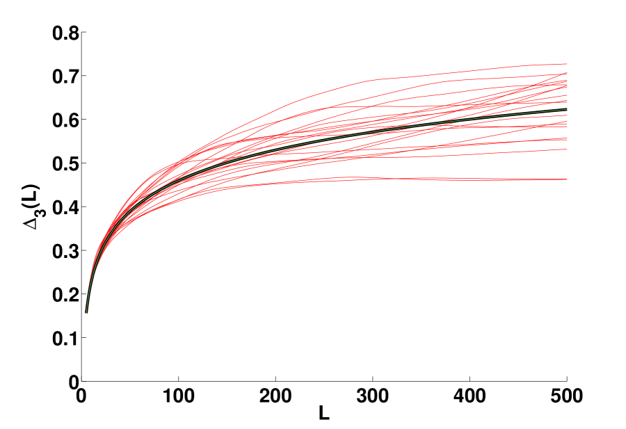
Figure 1: (Color online) Calculated $\Delta_{3}(L)$-statistic for an ensemble of 50 GOE spectra with $N=4000$, results for 20 spectra are shown as thin lines (red). The ensemble average, $\overline{\Delta_{3}(L)}$, for all the 50 spectra lies on the theoretical thick (black) curve, differing from it by $\approx 2\times 10^{-3}$ over the whole range of $L$.

To illustrate the problem, see Fig. 1, where $\Delta_{3}(L)$ is shown for 20 out of a set of 50 GOE spectra of random GOE matrices of dimension $N=4000$. Notice the lines tend to be quite smooth, but there is a considerable spread. The mean value of $\Delta_{3}(L)$ for these 50 spectra is shown in green in Fig. 1, but is not visible as it lies on the theoretical curve, Eq. (4). This average of the red lines is $\overline{\Delta_{3}(L)}$, the ensemble average of $\Delta_{3}(L)$. In this way we have recovered the theoretical result, the difference between theory and calculation $\approx 2\times 10^{-3}$ for the large range of $L$ shown. The source of the discrepancy for a specific spectrum is simply the natural spread in $\Delta_{3}(L)$ values for different spectra. This begs the question: if a $\Delta_{3}(L)$ calculation on some experimental data gave one of the lines in Fig. 1 what conclusions could be drawn about the purity of the spectra, missing levels, etc. We need an “uncertainty” to define a confidence interval centered on the theoretical line, so we can make meaningful comparisons with the data.

III Ergodicity of $\Delta_{3}(L)$

The validity of a comparison between the spectral average of a quantity with the theoretical ensemble average depends on the quantity being ergodic. For a clear and more detailed account of this topic see Brody et al. (1981).

Consider an observable $X(E)$, which is some function of energy. In RMT, this observable would be calculated by evaluating $X(E)$ for fixed $E$ and averaging over an ensemble of spectra to get the ensemble average, $\overline{X(E)}$. The variance of $X(E)$ is written $\text{Var}_{e}(X)=\overline{X(E)^{2}}-\overline{X(E)}\>^{2}$. We will write the standard deviation as $\sigma_{e}X$, or simply $\sigma_{e}$, the subscript indicating ensemble averaging. Dyson Dyson and Mehta (1963) derived the variance of $\Delta_{3}$ in GOE to be $\text{Var}_{e}(\Delta)=1.169/\pi^{4}=0.110^{2}$, so $\sigma_{e}=0.110$. On the other hand, experimentally one is dealing with an interval of the spectrum over an energy range (determined by the experiment) $[E,E+\Delta E]$, and one calculates the spectral average within that range, as a running average over the energy,

$$\langle X(E)\rangle=\frac{1}{\Delta E}\int^{E+\Delta E}_{E}X(E^{\prime})dE^{\prime}.$$ (5)

Ergodicity is equivalent to the statement $\langle X(E)\rangle=\overline{X(E)}$.

Take, for example, the nearest neighbor level spacing $s=E_{i+1}-E_{i}$. It is easy to verify that $s$ is ergodic, see Fig. 2. In this case the probability density for $s$ is the same within a spectrum as it is in the ensemble. The formal requirement for $X(E)$ to be ergodic is that $\text{Var}_{e}\langle X(E)\rangle=\overline{\langle X(E)\rangle^{2}}-\overline{\langle X(E)\rangle}\>^{2}\rightarrow 0$ as $\Delta E\rightarrow\infty$. As it stands it is not particularly useful, what we need is the behavior of $\text{Var}_{e}\langle X(E)\rangle$ for finite data sets. Specifically, we need an expression for the uncertainty in the quantity after replacing ensemble averaging with spectral averaging. We will refer to this quantity as $\sigma$, with $\text{Var}_{e}\langle X(E)\rangle=\sigma^{2}$.

In application to $\Delta^{i}_{3}(L)$, the energy dependence is in $i$, which indicates the location $E_{i}$ of the window of $L$ levels. The spread in the individual lines in Fig. 1 is $\sigma$, while their average is $\overline{\langle\Delta^{i}_{3}(L)\rangle}$, or $\overline{\Delta_{3}(L)}$, which is the notation we will use. It is $\sigma$ that will determine the sensitivity of $\Delta_{3}$ as a tool for detecting missing levels. In a calculation of $\Delta_{3}(L)$ on a spectrum of $N$ levels, we take a spectral average of $\Delta_{3}^{i}(L)$, where the average is taken over the $N-L$ possible locations $E_{i}$ of the window of $L$ levels. Brody et al. Brody et al. (1981) discuss the situation where a quantity $X$ is calculated over $p$ non-overlapping intervals. They suggest that $\text{Var}_{e}\langle X\rangle_{p}=\text{Var}_{e}(X)/p$. They call this the Poisson estimate. In the case of the $\Delta_{3}$ statistic, there are $N/L$ non-overlapping intervals available for each $L$, and the Poisson estimate would prescribe an uncertainty of $\sigma=0.11\sqrt{L/N}$. We will verify this numerically for the GOE. In practice the intervals used in the calculation overlap, as we allow $i$ to take all available $N-L$ values. The values of $\Delta_{3}^{i}(L)$ are highly correlated in this case however, and the Poisson estimate is still good. It is clear from this result that $\Delta_{3}$ is a more sensitive statistic for small values of $L/N$.

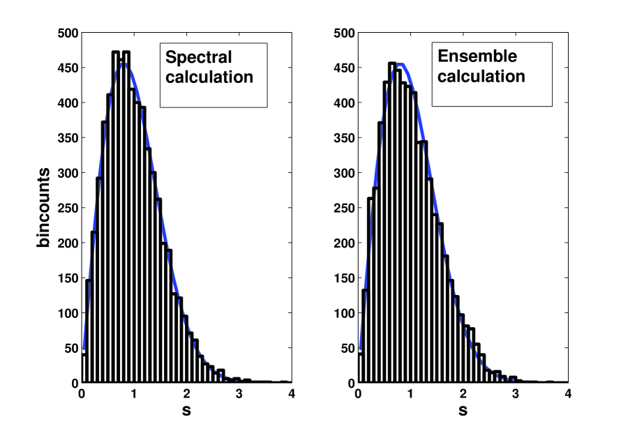
Figure 2: (Color online) The distribution of level spacings, $s$, taken from one $N=6000$ GOE spectrum, left, and the distribution of the center level spacing, $E_{300}-E_{299}$, taken from an ensemble of 6000 GOE spectra with $N=600$. The distributions are the same. The statistic $s$ is ergodic.

In the case of $m$ independent spectra, superimposed in proportions $f_{1},\,f_{2},\,\dots f_{m}$, and letting $\Delta_{3m}(L)$ be the spectral rigidity of the $m^{\textrm{th}}$ sub-spectrum, we have Dyson and Mehta (1963) $\Delta_{3}(L)=\sum_{i=1}^{m}\Delta_{3m}(f_{i}L)$. If the $m$ spectra are all from the GOE, the ensemble variance is $\sigma_{e}^{2}=(0.110\,m)^{2}$, and the Poisson estimate then gives $\sigma=0.110\,m\,\sqrt{L/N}$. Based on this number $\Delta_{3}(L)$ can be used to distinguish between spectra with $m=1$ and $m=2$ independent sequences present. However this statistic is not sensitive to the actual mixing fractions. We have assumed here that the proportions $f_{1},\,f_{2},\,\dots f_{m}$ are independent of energy. This may not be the case, in neutron resonances, the fraction of intruder p-wave resonances may grow with energy.

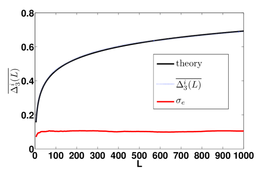
Figure 3: (Color online) The dotted (blue) curve is $\overline{\Delta^{i}_{3}(L)}$, the ensemble average of $\Delta^{i}_{3}(L)$, for $i=1200-\frac{L}{2}$; the ensemble of 1000 spectra with $N=2400$ was used. The ensemble average is indistinguishable from the RMT prediction, solid (black) line. The lower (red) curve is $\sigma_{e}$, the standard deviation of $\overline{\Delta^{i}_{3}(L)}$. It agrees with the RMT result of 0.11.

To calculate the ensemble average, $\overline{\Delta^{i}_{3}(L)}$, 1000 matrices of dimension 3000 were made. Each of these spectra was unfolded. The value of $i=\frac{N}{2}-\frac{L}{2}$ was chosen to locate the window of $L$ levels squarely in the middle of the spectrum, $\Delta_{3}^{i}(L)$ was calculated, and the resulting $\overline{\Delta^{i}_{3}(L)}$ matched the RMT result, see Fig. 3. As a double check, the process was repeated for the value of $i=\frac{N}{4}-\frac{L}{2}$, which locates the window of $L$ levels on the left edge of the spectrum. A discrepancy here would undermine our unfolding procedure, see Sec. IV, but the results were identical.

IV Calculation of $\Delta_{3}(L)$

To realize the GOE, we generated random matrices with normally distributed matrix elements, and

$$P(H_{i\neq j})=\frac{1}{\sqrt{2\pi\sigma^{2}}}\,e^{-\frac{H_{ij}^{2}}{2\sigma^{2}}},\quad P(H_{ii})=\frac{1}{\sqrt{4\pi\sigma^{2}}}\,e^{-\frac{H_{ii}^{2}}{4\sigma^{2}}}$$ (6)

for the off-diagonal and diagonal elements, respectively. We chose $\sigma=1$. Each of the matrices has an approximately semicircular level density, with $\rho(E)=\sqrt{4N-E^{2}},\;\text{for }|E|\leq 2\sqrt{N},\;0\text{ otherwise}$ (actually there are deviations from the semicircle at the edges, see Mehta Mehta (1991)).

In order to apply the results of RMT to real data, the empirical spectrum must be unfolded Guhr et al. (1998); Brody et al. (1981) separating the fluctuations of the spectra from secular behavior and expressing all energies in units of the local average level spacing. This is achieved by first extracting the cumulative level density ${\mathcal{N}}(E)$, which will be a staircase function, from the raw data, and fitting it to a smooth function, $\xi(E)$, either numerically, or analytically. Then, using this function, the $j^{th}$ level of the unfolded spectrum is simply $\xi(E_{j})$. The resulting unfolded spectrum has a uniform level density $\rho(E)=1$ so that data from high density regions can be compared with data from low density regions. Furthermore, spectra from very different physical systems can be compared.

Integrating the semicircular GOE level density gives

$$\xi(E) =\int_{-\infty}^{E}\rho(E^{\prime})dE^{\prime}$$ (7)

$$=\frac{1}{\pi}N~{}\tan^{-1}\left(\frac{E}{\sqrt{4N-E^{2}}}\right)+\frac{1}{4\pi}\,E\sqrt{4N-E^{2}}+\frac{1}{2}N.$$

To decide between using the analytical form, or a numerical fit, the curve fitting tool in MATLAB was used to get the best values for $a$, $b$, and $c$ in the parametrization

$$\xi(E)=a~{}\frac{1}{\pi}N\,\tan^{-1}\left(\frac{E}{\sqrt{4N-E^{2}}}\right)+b~{}\frac{1}{4\pi}E\sqrt{4N-E^{2}}+c~{}\frac{1}{2}N.$$ (8)

The result is, with 95% confidence bounds, $a=0.9992~{}(0.9992,0.9993)$, $b=1~{}(1,1.001)$,and $c=1~{}(1,1)$. Using these values for a test spectrum with $N=500$ made a difference in $\Delta_{3}(L)$ of $10^{-3}$ at $L=250$, so the theoretical (semicircle) result, Eq. (7), was used in all the calculations of $\Delta_{3}(L)$ for GOE spectra, without any fitting. To realize ensembles of GOE spectra of various spectrum size, $N$, we first made an ensemble of 3000 unfolded GOE spectra with dimension 3000. Getting a spectrum of size $N$ is now a matter of taking the middle $N$ eigenvalues from one of these. In what follows, all calculations are performed on unfolded spectra.

We rewrite for convenience the definition of $\Delta_{3}(L)$ for a spectrum:

$$\Delta_{3}(L)=\left\langle{\rm min}_{A,B}\;\frac{1}{L}\;\int^{E_{i}+L}_{E_{i}}dE^{\prime}\,[\;{\mathcal{N}}(E^{\prime})-AE^{\prime}-B]^{2}\;\;\right\rangle\>.$$ (9)

The integration is over a window of the spectrum, of length $L$ levels, starting at energy $E_{i}$, the $i^{th}$ level. Note that some authors choose the limits of integration to be $E_{i-\frac{L}{2}},E_{i+\frac{L}{2}}$. The integral is evaluated for every starting energy $E_{i}$, with $1\leq i\leq N-L$. $A$ and $B$ are chosen so as to minimize the integral for each position of the window of $L$ levels, i.e. for each value of $i$. The precise values of $A$ and $B$ will be given in terms of $E_{i}$, no numerical minimization is necessary.

Substituting ${\mathcal{N}}(E)=i,E_{i}\leq E<E_{i+1}$, into (9), our job is reduced to finding the mean of the quantity $\Delta_{3}^{i}(L)$. In evaluating

$$\Delta_{3}^{i}(L)=\frac{1}{L}\;\int^{E_{i}+L}_{E_{i}}dE^{\prime}\,[\;{\mathcal{N}}(E^{\prime})-AE^{\prime}-B]^{2}\;,$$

consider the integral between two adjacent levels,

$$\Delta_{3}^{i}(L)=\frac{1}{L}\;\sum^{i+L-1}_{j=i}\int^{E_{j}+1}_{E_{j}}dE^{\prime}\,(j-AE^{\prime}-B)^{2}=\frac{1}{L}\times(C+VA^{2}+WA+XAB+YB+ZB^{2}),$$ (10)

where

$$C = \sum^{i+L-1}_{j=i}j^{2}(E_{j+1}-E_{j}),$$

$$V = \frac{1}{3}(E_{i+L}^{3}-E_{i}^{3}),$$

$$W = \sum^{i+L-1}_{j=i}-j(E_{j+1}^{2}-E_{j}^{2}),$$

$$X = (E_{i+L}^{2}-E_{i}^{2}),$$

$$Y = \sum^{i+L-1}_{j=i}-2j(E_{j+1}-E_{j}),$$

$$Z = (E_{i+L}-E_{i}).$$

Using the constraints $\partial(\Delta_{3}^{i})/\partial A=0$ and $\partial(\Delta_{3}^{i})/\partial B=0$, we come to the following expressions for $A$ and $B$ that minimize $\Delta_{3}^{i}(L)$:

$$A=\frac{XY-2WZ}{4VZ-X^{2}},\quad B=\frac{WX-2VY}{4VZ-X^{2}}.$$ (11)

Given an unfolded spectrum, $\Delta_{3}(L)$ can be calculated exactly. Bohigas and Giannoni derived a similar expression for the case of $L=N-1$ in Bohigas and Giannoni (1975). It is interesting to note that many early investigations of $\Delta_{3}(L)$ deal with just this special case, and hence distinction between a spectral average and an ensemble average didn’t arise, there being only one value of the statistic per spectrum.

V Calculation of $\sigma(L)$

To calculate $\sigma$, the uncertainty for $\Delta_{3}(L)$ of a specific GOE spectrum, we take 1000 GOE spectra, each with $N$ levels, and calculate $\Delta_{3}(L)$ for each. $\sigma$ is the standard deviation of those 1000 numbers for each $L$, and this is what we should use as the uncertainty for $\Delta_{3}(L)$ for that value of $L$. In Fig. 4 we show the $\overline{\Delta_{3}(L)}$ and $\sigma$ for a range of $N$. The most important feature is that $\sigma<\sigma_{e}$ for small values of $L$. When $L=N$ then we have one number per spectrum, and $\sigma=\sigma_{e}$ as expected.

To compare different size spectra, we plot $\sigma$ vs. $L/N$, in Fig. 5. A numerical fit to the range $0\leq L/N\leq 0.2$ gives

$$\sigma=0.1126(L/N)^{0.5003}-0.0045\approx\sigma_{e}\sqrt{L/N}.$$

This is a verification of the Poisson estimate. The dashed line in Fig. 5 is $\sigma=\sigma_{e}\sqrt{L/N}$. The Poisson estimate was stated for the case of non-overlapping intervals. In Eq. (10) this would mean $i=1,\,L+1,\,2L+1,\dots$. In our calculations all values of $i$ were used, this is equivalent to doing $L$ sets of calculations for non-overlapping intervals, with the initial values of $i$ in each set going from 1 to $L$, and then taking the average of these $L$ numbers, so the Poisson estimate is still valid. Note that these “uncertainties” are not to be confused with any experimental uncertainty or computational issue. Given an unfolded data set, the $\Delta_{3}(L)$ statistic is calculated exactly, as was shown in Sec. IV.

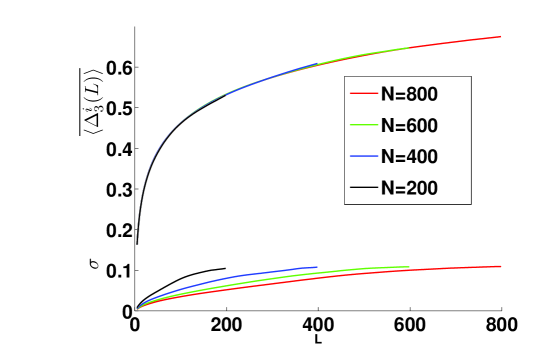
Figure 4: (Color online) The ensemble average, $\overline{\Delta_{3}(L)}$ vs. L is plotted for various values of $N$. Each ensemble had 1000 matrices. The lower lines are the standard deviations of the corresponding 1000 values of $\Delta_{3}(L)$. Notice that for the maximum value of $L$, $\sigma=0.11$, which is the ensemble result. This is expected, as there is only one such value per spectrum.

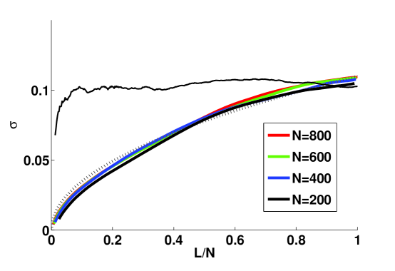
Figure 5: (Color online) Here we plot $\sigma$ from Fig. 4 vs. $L/N$, for various ensembles. The top (black) line is $\sigma_{e}$, in agreement with the RMT result of a constant 0.11 . The dashed line is $\sigma_{e}\sqrt{L/N}$.

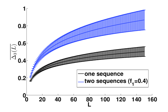
Figure 6: (Color online) $\overline{\Delta_{3}(L)}$ is plotted with uncertainties for the cases of an ensemble of 500 pure GOE spectra, lower lines (black), and a 500 mixed GOE spectra, upper lines (blue). In the mixed case, each spectrum was a superposition of 2 pure GOE spectra in proportions $f_{1}=0.4\,,f_{2}=0.6$. In both ensembles, the spectra had $N=500$. The uncertainties are empirical, being the standard deviation of the 500 values of $\Delta_{3}(L)$ at each value of $L$.

For the case of a mixture of $m=2$ independent GOE spectra, the ensemble result is $\sigma_{e}=0.22$. A calculation of $\sigma$ for 500 spectra each with 500 levels, made by mixing two GOE spectra, with $f_{1}=0.4$, gives $\sigma=0.239(L/N)^{0.522}-0.014$, which is consistent with $\sigma=2~{}\sigma_{e}\sqrt{L/N}$. In Fig. 6 we show $\Delta_{3}(L)$ with the empirical uncertainties. The statistic can clearly distinguish between $m=1$ and $m=2$ spectra, and it is most sensitive for small values of $L$. $\Delta_{3}(L)$ is not sensitive to the actual value of $f_{1}$, and cannot be used to distinguish between $f_{1}=0.25$ and $f_{1}=0.4375$. These are the values for the fraction densities one would expect for neutron resonances on target nuclei with spin $j_{{\rm tar}}=1/2$ and $7/2$, based on the $2j+1$ degeneracies of the resulting compound nucleus spins $j_{{\rm tar}}\pm 1/2$. The statistic is sensitive to $p$-wave neutrons in the beam being mislabeled as $s$-wave for spin-1/2 targets, as this would introduce multiple sequences of levels into the data set.

To determine the completeness of a spectrum with $\Delta_{3}(L)$, we need to know its behavior for GOE spectra with a fraction of levels, $x$, depleted. We denote this by $\Delta_{3}(L;x)$, and it was found empirically for ensembles of 500 spectra with dimension $N$ and depletion $x$. The dimension, $N$, refers here to the number of levels after the fraction $x$ was randomly removed. The ensemble average of $\Delta_{3}(L;x)$ and its standard deviation $\sigma(N,L;x)$ were calculated. The results are shown in Fig. 7 for $N=200$, with uncertainties. We see from Fig. 8 that the uncertainty here has the form $\sigma_{x}(N,L;x)=f(L)/\sqrt{N}$. The $1/\sqrt{N}$ dependence of $\sigma_{x}(N,L;x)$ means that the statistic is a less sensitive measure of $x$ for lower $N$. A fit to $f(L)$ was made for a range of $x$, to be used in practical analysis of the neutron resonance data.

Now we have the tools necessary to compare a real spectrum with depleted GOE spectra in a meaningful way. The best value for $x$ from the data will be the one that minimizes

$$\chi^{2}(x)=\sum^{L_{max}}_{L_{min}}\frac{[\Delta_{3}(L)-\Delta_{3}(L;x)]^{2}}{\sigma(N,L;x)^{2}}.$$ (12)

For practical purposes we need an estimate of the error in $x$ from this method. To this end, we calculated the average value of $x$, and its standard deviation, for 1500 GOE spectra with $N=100$ and 300 levels. The sets were made by randomly deleting 3 levels from a spectra of 103 levels, 5 out of 105, 9 out of 109, and 11 out of 111, to get spectra with $x=2.91\%$, 4.76%, 8.26%, and 9.9% respectively. The results are in Table 1. Our method gave good agreement for the value of $x$, but the uncertainties were of the same order as $x$, for example, with $x=4.76\%$, we get a value of $(4.89\pm 2.81)\%$. However, when we tried the method for $N=300$, the uncertainty dropped by a factor of nearly $\sqrt{3}$ to 1.66%, which is to be expected.

Table 1: The errors in $x$, the fraction of missed levels, using the $\Delta_{3}$ statistic. The tests were run for 1500 depleted spectra of size $N=100$ and 300. The mean value $\overline{x}$, and the standard deviation, $\sigma$ are given.

$x$	$\overline{x}\,(N=100)$	$\sigma\,(N=100)$	$\overline{x}\,(N=300)$	$\sigma\,(N=300)$
2.91%	3.14%	2.50%	2.71%	1.57%
4.76%	4.89%	2.81%	5.00%	1.66%
8.26%	7.95%	3.13%	7.94%	1.74%
9.91%	9.90%	3.06%	10.0%	1.77%

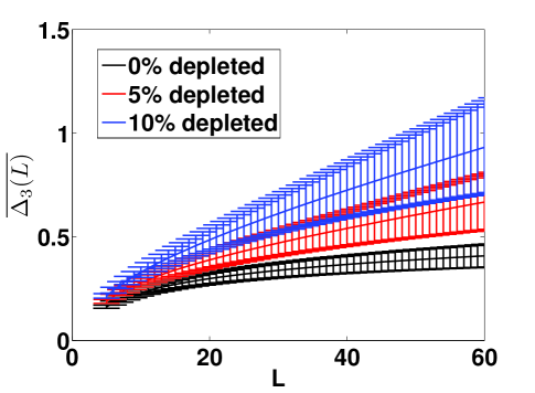
Figure 7: (Color online) $\overline{\Delta_{3}(L)}$ vs. $L$ is plotted for depleted spectra size, $N=200$, with uncertainties. Lower line has $x=0\%$ depletion, middle line has $x=5\%$, and the upper line has $x=10\%$.

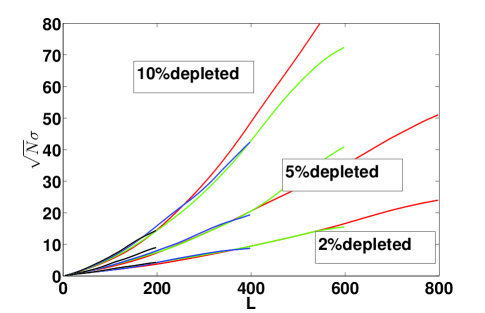
Figure 8: (Color online) $\sqrt{N}\sigma$ vs. $L$ is plotted for depleted spectra of dimension $N$. The values of $N$ are 200, 400, 600, and 800, $L$ goes out to its maximum value of $N-1$.

An experimental spectrum can be contaminated by intruder levels. In the case of $s$-wave neutron resonance data, this could be from the capture of $p$-wave neutrons. To examine the effect of contamination on $\Delta_{3}(L)$, ensembles of 1000 unfolded GOE spectra with $N=200(1-x)$ were made. Each spectrum was stretched by a factor of $1/(1-x)$ and then $200x$ random numbers, uniformly distributed on the interval $[0,200]$, were added. The resulting spectrum had a uniform level density, $\rho(E)=1$, a size $N=200$, and a level of contamination of $x\%$. In Fig. 9 we see the results for $x=2\%,\,5\%,\,\text{and}\;10\%$ (solid lines). The results agree well with the RMT prediction of $\Delta_{3}(L)=(1-x)[(\log L-0.0678)/\pi^{2}]+x\,L/15$ (dashed lines).

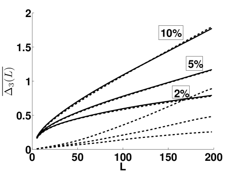
Figure 9: Here $\overline{\Delta_{3}(L)}$ is shown for contaminated GOE spectra, upper solid lines. The level of contamination, $x$, is labeled. Upper dashed lines are the RMT predictions. The dashed lines at the bottom of the plot are the standard deviations, $\sigma$, of $\Delta_{3}(L)$ for $x=2\%,\,\text{the lowest of the three, to}\,10\%,\,\text{the highest of the three}.$

We have discussed the spectral average of $\Delta^{i}_{3}(L)$, but what about its spread within a spectrum? We call the standard deviation of $\Delta^{i}_{3}(L)$ for a given spectrum $\sigma_{s}$. In Fig. 10 we see the average of $\sigma_{s}$ as a function of $L$ for different spectra sizes, $N$. It is immediately clear that $\sigma_{s}$ is less than $\sigma_{e}$. Within one spectrum, we expect a smaller spread in the values of $\Delta^{i}_{3}(L)$ because close values in $i$ mean the windows of $L$ levels overlap, the corresponding values of $\Delta^{i}_{3}(L)$ would be correlated, and $\sigma_{s}$ should get smaller as $L\rightarrow N$. A plot of $\sigma_{s}$ versus $L/N$ strongly suggests the falloff is linear, with $\sigma_{s}=\sigma_{e}(N-L)$, see Fig. 11. It is not obvious that the correlations between overlapping windows of levels would give this linear behavior. To gain insight into the correlation between $\Delta_{3}^{i}(L)$ and $\Delta_{3}^{i+1}(L)$, we examined the ensemble average of the square of the difference between these two quantities, specifically, $\delta\Delta(L)=\sqrt{\overline{[\Delta_{3}^{i+1}(L)-\Delta_{3}^{i}(L)]^{2}}}$, the variation of $\Delta_{3}^{i}(L)$ with respect to $i$. It is expected that this quantity should be closely related to $\Delta_{3}(L)$, and it certainly decreases rapidly, $\delta\Delta(L)\propto\Delta_{3}(L)/L$. The constant of proportionality is $\langle\frac{L\;\delta\Delta(L)}{\Delta_{3}(L)}\rangle_{L}=2.3303$, where the average was taken over all values of $L$, see Fig. 12.

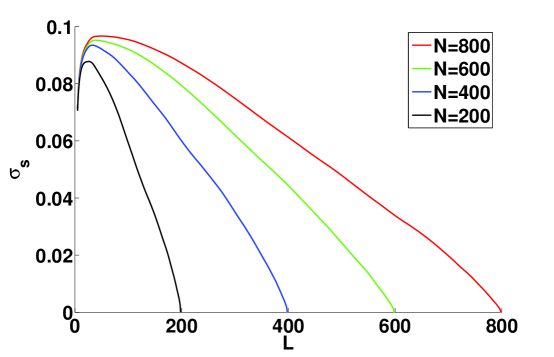
Figure 10: (Color online) The standard deviation of $\Delta_{3}^{i}(L)$ within a spectrum, $\sigma_{s}$, vs. $L$ is plotted for various values of $N$. The linear parts of the plot are well described by $\sigma_{s}=\sigma_{e}(N-L)$

.

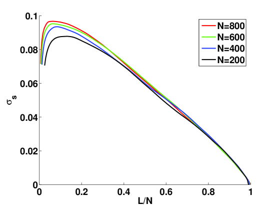
Figure 11: (Color online) $\sigma_{s}$ vs. $L/N$ is plotted for various values of $N$. The linear parts of the plot are well described by $\sigma_{s}=\sigma_{e}(1-L/N)$

.

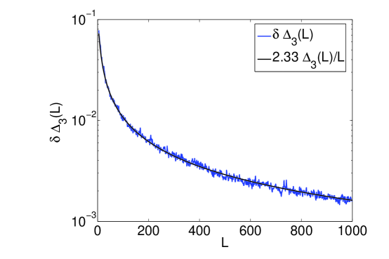
Figure 12: (Color online) The quantity $\delta\Delta(L)$, as defined in the text, is plotted on a log-linear graph. It is well approximated by $2.3303\Delta_{3}(L)/L$ (smooth line).

It is interesting to see the behavior of $\sigma_{s}(N,L;x)$, the spectral average of the variation of $\Delta_{3}(L;x)$. It has a strong $N$- and $x$-dependence, and the simple rule $\sqrt{N-L}$ of the $x=0$ case is lost. In Fig. 13 we show that the $N$-dependence of $\sigma_{s}(N,L;x)$ for 5% depletion peaks at $L\approx N/2$. Strong correlation in overlapping windows $L$ levels wide would reduce this number as $L$ increases, and in Fig. 14 the results for $N=200$ and $x=0\%,\,2\%,\,5\%,$ and $10\%$ show that the maximum moves to higher values of $L$ as $x$ increases.

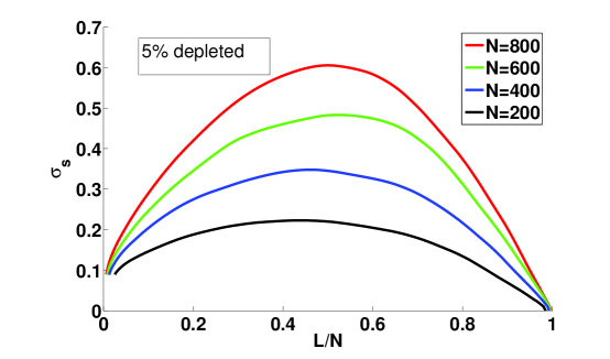
Figure 13: (Color online) The rescaled standard deviations for systems of various sizes, $\sigma_{s}(N,L;x)$, with 5% of levels depleted. Each line represents the average for 500 systems of a particular size.

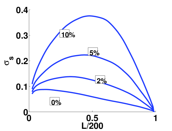
Figure 14: (Color online) The rescaled standard deviations for $N=200$, $\sigma_{s}(N,L;x)$, with varying degrees of depletion. Each line represents the average of 500 systems.

VI Level Spacing analysis

The nearest level spacing distribution can be used to test for missing levels, and mixing of different sequences. Here we will follow the work of Agvaanluvsan et al. Agvaanluvsan et al. (2003), where the maximum likelihood method is used to find the fraction of missing levels in a sequence. We will test the method on GOE spectra depleted by hand. Single sequence neutron resonance data will then be analyzed, and the results compared with those of a $\Delta_{3}$ analysis.

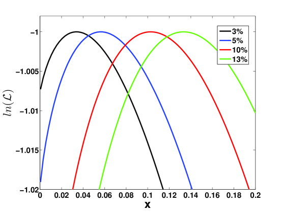
Figure 15: (Color online) The maximum likelihood method (MLM) is tested on a superposition of 200 GOE spectra, each of length $N=250$. A fraction $x$ of each spectrum was randomly removed, and the MLM was used to recover the number. Here are the results. The MLM slightly overestimates the fraction missing. The natural log of the likelihood function, $\ln({\mathcal{L}})$, is plotted against $x$.

The level spacing distribution for a complete GOE spectrum is given by the Wigner surmise,

$$P(s)=\frac{\pi}{2}se^{-\pi s^{2}/4},$$ (13)

where $s=S/D$, $S$ being the spacing between adjacent levels, and $D$ is the average spacing. We have unfolded all spectra involved, so $D=1$. If a level is missing, then two nearest neighbor spacings are unobserved, while one next-to-nearest spacing is included as a nearest level spacing, when it should not be. Furthermore, if $1-x$ is the fraction of the spectrum that is observed, then $D_{{\rm obs}}$, the experimental value for the average spacing, is related to the true value by $D=(1-x)D_{{\rm obs}}$. Agvaanluvsan et al. show that

$$P(s)=\sum_{k=0}^{\infty}(1-x)x^{k}P(k;s),$$ (14)

where $P(k;s)$ is the distribution function for the $k^{th}$ nearest neighbor spacing, $E_{k+i}-E_{i}$; for $k=0$ this reduces to the Wigner distribution, $P(0;s)=P(s)$.

The maximum likelihood method will be used to find the best value for $x$ that maximizes the likelihood function ${\mathcal{L}}=\prod_{i}P(s_{i})$; the product is over all the observed spacings. In practice it is easier to maximize $\ln({\mathcal{L}})=\sum_{i}\ln P(s_{i})$. The functions $P(k;s)$ are complicated to derive. For $k\neq 0$, the functions were fitted to the empirical distributions from the superposition of 5000 GOE spectra, each of length $N=5000$. The procedure was tested on 200 GOE spectra, each of length $N=250$, with 3%, 5%, 10% and 13% of levels randomly removed. The results are shown in Fig. 15. The method systematically overestimated $x$ by about 0.5%.

Table 2: The errors in $x$, the fraction of missed levels, using the maximum likelihood method. The tests were run for 1500 depleted spectra of size $N=100$ and 300. The mean value $\overline{x}$, and the standard deviation, $\sigma$ are given.

$x$	$\overline{x}\,(N=100)$	$\sigma\,(N=100)$	$\overline{x}\,(N=300)$	$\sigma\,(N=300)$
2.91%	3.32%	2.42%	3.44%	1.49%
4.76%	5.02%	2.56%	5.29%	1.43%
8.26%	8.45%	2.48%	8.74%	1.32%
9.91%	10.09%	2.33%	10.32%	1.18%

In order to get an estimate of the error in $x$ from this method, the procedure of the previous section was repeated, and the results are shown in Table 2. The agreement with the $\Delta_{3}(L)$ method is encouraging. The $\Delta_{3}(L)$ method seems to be slightly more accurate, but the uncertainty in $x$ is slightly smaller for the MLM.

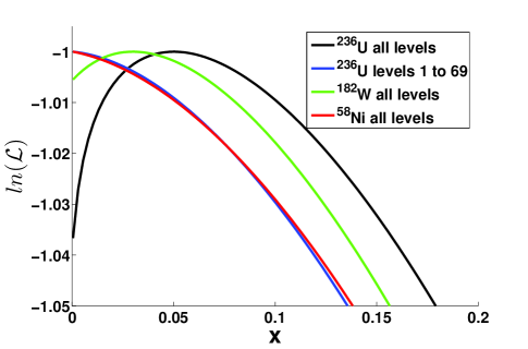
Figure 16: (Color online) MLM results are shown for some representative data sets. The indication is that the ${}^{236}\text{U}$ data is incomplete, with 5% of levels missing, but the subset of the data consisting of the first 69 levels looks complete. There appears to be 3% of levels missing from the ${}^{182}\text{W}$ data, with 0% missed from the ${}^{58}\text{Ni}$ data.

Next the procedure was applied to the real neutron resonance data. The data sets are described in the next section. In Fig. 16 we see some typical results of the MLM analysis. For the ${}^{236}\text{U}$ data, the full set of 81 levels looked incomplete, to the tune of about 5%, while the first 69 levels looked complete. The ${}^{182}\text{W}$ data looked like there were 3% of the 68 levels missing, while the 63 levels in the ${}^{58}\text{Ni}$ data looked like a complete set.

VII Neutron resonance data

The neutron resonance data for a wide range of isotopes are now widely available . Data sets with spin-0 target nuclei were chosen for analysis. They afforded the simplicity of not having the fractional densities $f_{1}$ and $f_{2}$ of a superposition of two independent spectra, as all levels have spin 1/2. There is a conventional assumption here that the capture is dominated by $s$-wave neutrons, so no higher angular momentum resonances intrude. Eleven isotopes were analyzed, and the data sets are described in Table 3.

The cumulative level number gives the first indication of the purity of the data. Kinks in ${\cal N}(E)$ leading to smaller slopes would suggest a section of data where levels were missing. Using this as a guideline, some data sets were split into subsets. For example, in Fig. 17 there is a kink in ${\cal N}(E)$ at the $70^{\text{th}}$ level, so we analyzed the subset of levels $E_{1}\rightarrow E_{70}$. The percentage of missing levels was estimated with the maximum likelihood method. $\Delta_{3}(L)$ was then calculated for each set, and compared with the MLM results. In Fig. 17 the three quantities are shown for two representative isotopes, ${}^{154}\text{Gd}$ (blue), and ${}^{152}\text{Gd}$ (red). The results are summarized in Table 3. The agreement between the two methods is promising.

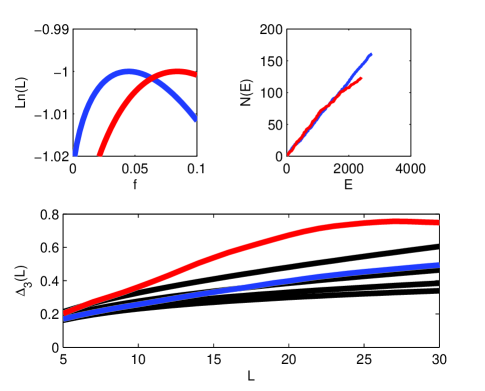
Figure 17: (Color online) $\Delta_{3}(L)$ vs. $L$ for the experimental data. The black lines are the GOE values for 0%, 2%, 5%, and 10%, starting from the lowest curve. The ${}^{154}\text{Gd}$ data is in blue, and the ${}^{152}\text{Gd}$ data is in red.

Table 3: The results for $x$, the percent of missing levels in the data.

Isotope	MLM	$\Delta_{3}(L)$	N (# levels)	subset
${}^{50}\text{Cr}$	2%	4%	64	$1\rightarrow 36$
${}^{50}\text{Cr}$	0%	8%	64	$37\rightarrow 64$
${}^{54}\text{Fe}$	3%	0%	63	$1\rightarrow 50$
${}^{58}\text{N}$	0%	0%	63	All
${}^{152}\text{Sm}$	3%	2%	91	$1\rightarrow 70$
${}^{152}\text{Gd}$	8%	12%	128	$1\rightarrow 70$
${}^{154}\text{Gd}$	4%	2%	161	All
${}^{158}\text{Gd}$	11%	7%	93	All
${}^{158}\text{Gd}$	0%	1%	93	$1\rightarrow 60$
${}^{158}\text{Gd}$	12%	15%	93	$61\rightarrow 93$
${}^{182}\text{W}$	3%	2%	68	All
${}^{234}\text{U}$	6%	4%	118	$1\rightarrow 75$
${}^{234}\text{U}$	7%	3%	118	$76\rightarrow 118$
${}^{234}\text{U}$	9%	8%	118	All
${}^{236}\text{U}$	0%	1%	81	$1\rightarrow 69$
${}^{236}\text{U}$	5%	8%	81	All
${}^{240}\text{Pu}$	0%	3%	267	$1\rightarrow 100$
${}^{240}\text{Pu}$	8%	12%	267	$171\rightarrow 267$
${}^{242}\text{Pu}$	11%	13%	67	All

There is a range of behaviors exhibited by $\Delta_{3}(L)$. It can be flatter than the RMT value, which suggests an artificially rigid spectrum. This type of behavior is typical when the unfolding procedure employs too specific a function for ${\cal N}(E)$, and all the fluctuations are washed out, leaving the unfolded spectrum too rigid. It can grow too rapidly, which could mean that there are more independent spectra present than thought. This would happen if, for example, $p$-wave neutrons were contributing to the data.

In the presence of sequences of energy levels with different spin labels, we would have a superposition of independent spectra. This is the case, for example, when $s$-wave neutrons are incident on a target nucleus with spin $j_{{\rm tar}}$, so that the resulting resonances have spin $j_{\pm}=j_{{\rm tar}}\pm\frac{1}{2}$. The level density is relatively constant over the small energy range of the data, and one would naively expect that the subspectra have fractional densities $f_{1}=\frac{2j_{-}+1}{(2j_{-}+1)+(2j_{+}+1)}$ and $f_{2}=1-f_{1}$. For $m$ independent spectra, with fractional densities $f_{1}\,,f_{2}\dots f_{m}$, and letting $\Delta_{3m}(L)$ be the spectral rigidity of the $m^{\rm{th}}$ sub-spectrum, we have $\Delta_{3}(L)=\sum_{i=1}^{m}\Delta_{3m}(f_{i}L)$.

A preliminary analysis of systems of mixed independent spectra was done on the ${}^{235}\text{U}$ data Leal et al. (1997). The $s$-resonances have spins $j=3$ and 4, making the data a superposition of two independent spectra, with $f_{1}=0.4325$. This data set exhibited all the behaviors described above. This data set, the biggest by far, was split into four sections corresponded to linear regions on the ${\cal N}(E)$ curve. The data was unfolded by fitting sections of ${\cal N}(E)$ to a straight line. The first section had 950 levels and the energy range from 0 to 510 eV. It exhibited excellent agreement with the GOE result for mixed ($f_{1}=0.4$) spectra with 4% depletion. The next sets were levels 1050 to 1450, with range $578~{}\text{eV}\rightarrow 920~{}\text{eV}$, 1700 to 2700 with range $1118~{}\text{eV}\rightarrow 1995~{}\text{eV}$, and the fourth set had levels 2750 to 3150, with range $2022~{}\text{eV}\rightarrow 2240~{}\text{eV}$. The results are summarized in Fig. 19. Although we do not have a MLM comparison for the case of two independent spectra, the $\Delta_{3}(L)$ analysis suggests that 4% of the levels were missing in the first 960 levels.

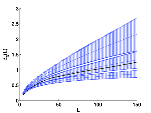
Figure 18: (Color online) $\Delta_{3}(L)$ vs. $L$ is plotted for the first 960 levels of the ${}^{235}\text{U}$ data. The uncertainties are empirical for mixed ($f_{1}=0.44$) GOE spectra, with 0%, 4%, and 10$ depleted. The data is consistent with there being 4% of levels missing.

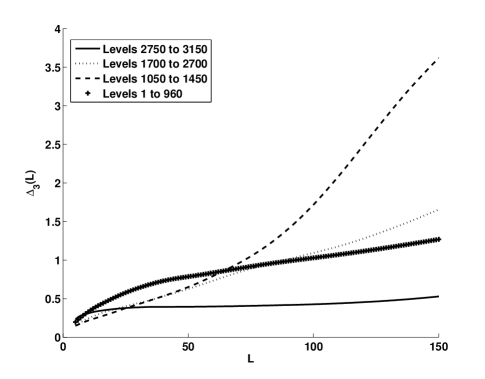
Figure 19: $\Delta_{3}(L)$ vs. $L$ is plotted for the four subsets of the ${}^{235}\text{U}$ data.The plot suggests that the middle sections of the data are less pure than the first set, but the highest energy set looks artificially rigid, like a harmonic oscillator spectrum.

VIII Conclusion

We have reexamined the possibility of using the Dyson-Mehta $\Delta_{3}(L)$ statistic as a diagnostic for the spectra of quantum systems in the chaotic regime, where the fluctuations can be modeled by Random Matrix Theory. Originally it was regarded as a tool of much more limited resolution, due to the large variance Dyson and Mehta (1963). This is not the full picture, and the definition of the statistic and the original results are reinterpreted. An examination of the ergodicity of the statistic lead to the spectral properties being separated from ensemble properties. We see that it is inappropriate to use the large and constant variance of the statistic as an uncertainty. Uncertainties in $\Delta_{3}(L)$ were found empirically for pure and depleted GOE spectra. In doing this, the Poisson estimate of Brody et al. was verified. The $\Delta_{3}(L)$ statistic was used to determine the percentage of missing levels in neutron resonance data. The results were compared with the maximum likelihood method of Agvaanluvsan et al Agvaanluvsan et al. (2003), and the agreement was good. The method was applied to ${}^{235}\text{U}$ data with curious results. Various sections of the data displayed different behavior, raising questions about the purity of the data, the accuracy of the angular momentum assignment, and the appropriateness of the modeling the data with RMT. The behavior of $\sigma_{s}$, the spectral spread of $\Delta^{i}_{3}(L)$, was examined, and new properties were described which need a more detailed study. It is hoped that the $\Delta_{3}(L)$ statistic will be considered as a useful diagnostic in the RMT arsenal for data analysis.