Breit type equation for mesonic atoms

Abstract

The finite size effects and relativistic corrections in pionic and kaonic hydrogen are evaluated by generalizing the Breit equation for a spin-0 - spin-1/2 amplitude with the inclusion of the hadron electromagnetic form factors. The agreement of the relativistic corrections to the energies of the mesonic atoms with other methods used to evaluate them is not exact, but reasonably good. The precision values of the energy shifts due to the strong interaction, extracted from data, are however subject to the hadronic form factor uncertainties.

More than fifty years after their first appearance camac , hadronic atoms continue to be important for a better understanding of fundamental interactions. One of the first speculations of their existence came from the historic papers of Fermi, Teller and Wheelerwheel , where they showed that the time required for a negative meson (they were actually referring to muons) to be trapped into an atomic orbit would be ($\sim 10^{-13}$ s) much less than its mean weak decay lifetime ($\sim 10^{-6}$ s). The negative hadron which is generally trapped into an excited state, undergoes transitions to lower states until it eventually enters the field of the nuclear strong interaction. The energy levels and widths of the hadronic atomic states are naturally affected by the strong interaction and hence experimental programmes to measure the shifts in the energies and widths in pionic piexp ; piothers , kaonic dear , $\Sigma$-hyperonic, antiprotonic and pionium sigexp atoms accurately are being carried out vigorously with the aim of pinning down the strong interaction parameters. However, the extraction of these parameters to a good accuracy, requires the determination of the electromagnetic corrections accurately too. For example, the availability of precision data on pionic hydrogen piexp and deuterium pidatom has led to calculations of various electromagnetic corrections to the hadronic scattering lengths to better than 1$\%$ sigg ; eric .

Whilst most of the calculations in recent literature aim at a high accuracy in evaluating corrections such as those due to vacuum polarization, relativistic recoil and other higher order corrections, the finite size of the pion and the proton is treated in a rather simplistic way. The correction to the binding energy of the pionic hydrogen, due to the extended charge of the pion and the proton is given in some works as lyubov ,

$$\Delta E={2\over 3}\,\mu^{3}\,\,\alpha^{4}\,\,\biggl{[}\langle r_{\pi}^{2}\rangle\,+\,\langle r_{p}^{2}\rangle\biggr{]}\,,$$ (1)

where, $\mu$ is the reduced mass of the $\pi p$ system, $r_{\pi}$ and $r_{p}$ the charge radii of the $\pi$ and $p$ respectively and $\alpha$ the usual fine structure constant. In sigg , the Coulomb potential was modified by introducing a Gaussian charge distribution which depended on the pion and proton charge radii. In the present work, we evaluate the relativistic and finite size corrections (FSC) by modifying the Breit equation lali4 to include the meson (pion or kaon) and the proton electromagnetic form factors. For similar Breit-like approaches, see breitlike . The results of this Breit type equation approach are compared with an ‘improved Coulomb potential’ austen which has been used in sigg ; piexp , to obtain corrections due to relativistic recoil and the anomalous magnetic moment of the proton, while extracting the strong energy shift in pionic hydrogen. Using the available parameterizations of the hadron form factors, we also investigate the uncertainty in the estimate of the FSC. Considering the high precision with which the strong energy shifts and widths for the $1s$ pionic hydrogen states, namely, $\epsilon_{1s}=-7.108\pm 0.013$ (stat) $\pm 0.034$ (syst) eV and $\Gamma_{1s}=0.868\pm 0.040$ (stat) $\pm 0.038$ (syst) eV piexp , as well as the hadronic $\pi N$ scattering length, $a_{\pi^{-}p}^{h}=0.0870(5)$ m${}_{\pi}^{-1}$ eric are being quoted and the accuracy with which the one loop calculations for the ground state energy of the pionic hydrogen are carried out gasser , the present results become relevant.

There is no unique approach to calculate relativistic corrections to level shifts of bound two-body systems breitlike ; austen ; pilkuhn1 . We shall employ the technique of the Breit equation as it is particularly suited to include form-factors effects in a rather transparent way. This way an equation emerges which combines relativistic and finite size (FSC) effects. A further motivation to use the Breit approach is to compare it with results obtained in a different way. Regarding the relativistic corrections, it is known that the Breit equation is consistent at the order $\alpha^{4}$ pilkuhn2 and using first order time-independent perturbation theory to calculate the energy corrections pilkuhn3 . The presence of negative energy states poses a problem in perturbation theory at higher orders pilkuhn3 . A detailed comparison between the results obtained in the Breit framework and an equation which correctly projects the positive energies has been performed in salp . The correction to the Breit energy in this work is given as, $\Delta E_{cc}=-2\alpha^{5}\mu^{3}/3\pi M_{\pi}M_{p}$ ($\mu$ is the reduced mass, $M_{\pi}$ the pion and $M_{p}$ the nucleon mass) which applied to pionic atoms gives $6\times 10^{-5}$ eV. This is too small to be of relevance here.

To evaluate the complete electromagnetic potential, we expand the amplitude for $\pi p$ elastic scattering, in $1/c^{2}$ terms, thereby generalizing the Breit type equation lali4 by the inclusion of the proton and pion electromagnetic form factors. This leads to non-local terms in the potential, whose contributions are not negligible weold . The $p\gamma p$ and the $\pi^{-}\gamma\pi^{-}$ vertices can be written in terms of the form factors $F_{1}^{p}$, $F_{2}^{p}$ (representing the charge and magnetization distributions in the proton) and $F^{\pi}$ (charge distribution in the pion) as,

$$\Gamma_{p}^{\mu} = F_{1}^{p}\,\gamma^{\mu}\,\,-\,\,{\sigma^{\mu\nu}\over 2M_{p}\,c}\,q_{\nu}\,F_{2}^{p}$$ (2)

$$\Gamma_{\pi}^{\nu} = F^{\pi}(q^{2})\,(P_{2}+P_{2}^{\prime})^{\nu}\,,$$

The photon four-momentum, $q=P_{1}^{\prime}-P_{1}=P_{2}-P_{2}^{\prime}$. In the non-relativistic limit ($q^{0}=0$) and $q^{2}=-\vec{Q}^{2}$, where, $\vec{Q}=\vec{p}_{1}^{\,\,\prime}-\vec{p}_{1}=\vec{p}_{2}-\vec{p}_{2}^{\,\,\prime}$.

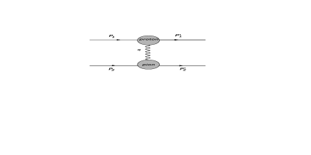
Figure 1: Feynman diagram for pion-proton scattering

The amplitude for the process $\pi^{-}+p\rightarrow\pi^{-}+p$ is given by weold ,

$$M_{fi}=-\alpha[\,(\bar{u}(\vec{p}_{1}^{\,\,\prime})\,\Gamma_{p}^{\mu}\,u(\vec{p}_{1}))\,\,D_{\mu\nu}(\vec{Q})\,\,\Gamma_{\pi}^{\nu}]\,(1/\sqrt{2E_{2}/c}\,)\,(1/\sqrt{2E_{2}^{\prime}/c}\,),$$ (3)

where, $D_{\mu\nu}(\vec{Q})$ is the photon propagator and $u(\vec{p}_{1})$, $u(\vec{p}_{1}^{\,\prime})$, the Dirac spinors given as, $u=\sqrt{2M}[(1-{\vec{p}^{\,2}\over 8M_{p}^{2}c^{2}})\,w),{\vec{\sigma}\cdot\vec{p}\over 2M_{p}c}\,w)]^{T}$. Substituting for the $u(\vec{p})$’s and the vertex factors, $\Gamma^{\mu}_{p}$ and $\Gamma^{\nu}_{\pi}$, the amplitude in (3) is evaluated and then rearranged to be written in the form,

$$M_{fi}=-2\,M_{p}\,[w_{1}^{\prime*}\,\,U(\vec{p}_{1},\vec{p}_{2},\vec{Q})\,w_{1}\,]\,,$$ (4)

thus obtaining the potential in momentum space: $U(\vec{p}_{1},\vec{p}_{2},\vec{Q})=-4\pi\,\alpha\,\sum_{i}\,\,U_{i}(\vec{p}_{1},\vec{p}_{2},\vec{Q})$, where,

$$U_{1} = {F_{1}^{p}(Q^{2})\,F^{\pi}(Q^{2})\over Q^{2}}\,,\,\,\,U_{2}=-\,{F^{\pi}(Q^{2})\,F_{2}^{p}(Q^{2})\over 4\,M_{p}^{2}\,c^{2}}\,,\,\,U_{3}=-\,{F_{1}^{p}(Q^{2})\,F^{\pi}(Q^{2})\over M_{p}\,M_{\pi}\,c^{2}\,Q^{2}}\,\biggl{[}\,\vec{p}_{1}\cdot\vec{p}_{2}\biggr{]}\,,$$

$$U_{4} = \,{F_{1}^{p}(Q^{2})\,F^{\pi}(Q^{2})\over M_{p}\,M_{\pi}\,c^{2}\,Q^{2}}\,\,\biggl{[}{(\vec{p}_{1}\cdot\vec{Q})\,(\vec{p}_{2}\cdot\vec{Q})\over Q^{2}}\,\biggr{]}\,,\,\,U_{5}=-\,{F^{\pi}(Q^{2})\,F_{1}^{p}(Q^{2})\over 8\,M_{p}^{2}\,c^{2}}$$ (5)

$$U_{6} = -\,{F_{1}^{p}(Q^{2})\,F^{\pi}(Q^{2})\over 2\,M_{p}\,M_{\pi}\,c^{2}\,Q^{2}}\,[\,i\,(\vec{\sigma}_{1}\times\vec{Q})\cdot\vec{p}_{2}\,]\,,\,\,\,U_{7}=-{F_{2}^{p}(Q^{2})\,F^{\pi}(Q^{2})\over 2\,M_{p}\,M_{\pi}\,c^{2}\,Q^{2}}\,[i\,(\vec{\sigma}_{1}\times\vec{Q})\cdot\vec{p}_{2}]$$

$$U_{8} = {F_{1}^{p}(Q^{2})\,F^{\pi}(Q^{2})\over 4\,M_{p}^{2}\,c^{2}\,Q^{2}}\,[i\,\vec{\sigma}_{1}\,\cdot(\vec{Q}\times\vec{p}_{1})]\,,\,\,\,U_{9}={F_{2}^{p}(Q^{2})\,F^{\pi}(Q^{2})\over 2\,M_{p}^{2}\,c^{2}\,Q^{2}}\,[i\,(\vec{p}_{1}\times\vec{\sigma}_{1})\cdot\vec{Q}]\,.$$

The potential in $r$-space is got by Fourier transforming each of the above terms lali4 , namely,

$$V_{i}(\vec{p}_{1},\vec{p}_{2},\vec{r})\,=\,\int\,e^{i\vec{Q}\cdot\vec{r}}\,\,U_{i}(\vec{p}_{1},\vec{p}_{2},\vec{Q})\,\,{d^{3}Q\over(2\,\pi)^{3}}\,\,.$$ (6)

The vectors $\vec{p}_{1}$ and $\vec{p}_{2}$ become differential operators in $r$-space lali4 . The FSC to the $1s$ state in pionic hydrogen can now be calculated as, $\Delta E={\alpha\over a}\,+\,\sum_{i}\Delta E_{i}$, where,

$$\Delta E_{i}=\int\Psi_{100}(r)\,\,V_{i}(\vec{p}_{1},\vec{p}_{2},r)\,\,\Psi_{100}(r)\,d\vec{r}$$ (7)

and $\Psi_{100}(r)=e^{-r/a}/(\sqrt{\pi\,a^{3}})$ with the Bohr radius $a=1/\alpha\mu$ and $\mu$ the $\pi p$ reduced mass. The factor $\alpha/a$ in $\Delta E$, arises from the fact that the potential $V_{1}(\vec{p}_{1},\vec{p}_{2},r)$ contains the usual ($1/r$) Coulomb potential too which must be subtracted while calculating $\Delta E_{1}$. The spin-dependent terms ($U_{6}$ to $U_{9}$) do not contribute to $\Delta E$ for the $1s$ state (see the appendix of weold ). Expressing $F_{1}^{p}$ and $F_{2}^{p}$, in terms of the Sachs form factors weold , $G_{E}^{p}(Q^{2})$ and $G_{M}^{p}(Q^{2})$ and using Eqs (Breit type equation for mesonic atoms, 6 and 7), the total $\Delta E$ is given as a sum of the terms:

$$\Delta E_{12} = \biggl{(}\,{\alpha\over a}\,+\,\Delta E_{1}\,\biggr{)}\,+\,\Delta E_{2}=-{32\,\alpha\over\pi\,a^{4}}\,\int_{0}^{\infty}\,{F^{\pi}(Q^{2})\,G_{E}^{p}(Q^{2})\,dQ\over(a^{\prime 2}+Q^{2})^{2}}\,+\,{\alpha\over a}$$ (8)

$$\Delta E_{34} = \Delta E_{3}+\Delta E_{4}={16\,\alpha\over\pi\,M_{p}\,M_{\pi}\,a^{5}}\,\int_{0}^{\infty}\,{F_{1}^{p}(Q^{2})\,F^{\pi}(Q^{2})\over Q^{2}}\,\biggl{[}\,{tan^{-1}(Qa/2)\over Q}\,-\,{a^{\prime}\over a^{\prime 2}+Q^{2}}\,\biggr{]}\,dQ$$

$$\Delta E_{5} = {4\,\alpha\over\pi\,M_{p}^{2}\,a^{4}}\,\int_{0}^{\infty}\,F_{1}^{p}(Q^{2})\,F^{\pi}(Q^{2})\,{Q^{2}\over(a^{\prime 2}+Q^{2})^{2}}\,dQ\,,$$

with, $a^{\prime}=2/a$. In the above, the individual contribution due to $\Delta E_{2}$ is found to be much smaller than $(\alpha/a)+\Delta E_{1}$ and in fact the two expressions can be combined to be written in the above compact form for $\Delta E_{12}$. The term $U_{3}$ in (Breit type equation for mesonic atoms) gives rise to the correction $\Delta E_{3}$ which cancels exactly with part of the term arising from $\Delta E_{4}$ and hence we write the total sum of these two terms above as $\Delta E_{34}$. Putting $F_{1}^{p}=G_{E}^{p}=F^{\pi}=1$ in (8), i.e. in the case of point hadrons, one gets from (8) the Coulomb term plus relativistic corrections.

We use two forms for the form factors of the proton. In the standard dipole form, $G_{E}^{p}(Q^{2})\simeq G_{M}^{p}(Q^{2})/\mu_{p}\simeq G_{D}(Q^{2})$, with, $G_{D}(Q^{2})=1/(1\,+\,Q^{2}/m^{2})^{2}$, $m^{2}=0.71$ GeV² and $\mu_{p}$ the magnetic moment of the proton. The other parameterization is one of the latest phenomenological fit walch , where, $G_{E}^{p}$ and $G_{M}^{p}$ are given by the ansatz, $G_{N}(Q^{2})=G_{S}(Q^{2})+a_{b}\,Q^{2}\,G_{b}(Q^{2})$. The explicit forms of $G_{S}(Q^{2})$ and $G_{b}(Q^{2})$ are given in walch and the parameters for the proton form factors are given in Table II of walch . The existing data amendolia ; piffdata on the pion form factor is well reproduced by a monopole form, namely,

$$F^{\pi}(Q^{2})\,=\,{1\over 1\,+\,(\langle r_{\pi}^{2}\rangle/6)\,Q^{2}}\,=\,{\Lambda_{\pi}^{2}\over\Lambda_{\pi}^{2}\,+\,Q^{2}}$$ (9)

such that, $\Lambda_{\pi}^{2}=6/\langle r_{\pi}^{2}\rangle$. The corrections (8) can be evaluated analytically, using the dipole form of the proton form factors. Since the analytic expressions for $\Delta E$ are lengthy, we give below, only the leading terms (in $\alpha$) of each of these terms. The sum of the corrections using $U_{1}$ and $U_{2}$ is denoted as $\Delta E^{lead}_{12}$, that coming from $U_{3}$ and $U_{4}$ in (Breit type equation for mesonic atoms) as $\Delta E^{lead}_{34}$ and one arising due to $U_{5}$ as $\Delta E^{lead}_{5}$.

$$\Delta E^{lead}_{12} = \biggl{(}{16\,\alpha\,m^{4}\,\Lambda_{\pi}^{2}\,\over a^{3}}\,\biggr{)}\,\,\biggl{[}{2\,M_{p}^{2}\,d_{1}\over m_{13}}\,+\,{3M_{p}^{2}\,d_{2}\over m_{13}^{2}}\,-\,{\Lambda_{\pi}^{2}\,d_{2}\over 4m_{13}^{2}}\biggr{]}\,,$$ (10)

$$\Delta E^{lead}_{34} = {8\,\alpha\,\Lambda_{\pi}^{2}\,m^{4}\,M_{p}\over M_{\pi}\,a^{3}}\,\,d_{3}\,-\,{4\,\alpha\,M_{p}\,m^{4}\,\Lambda_{\pi}^{2}\over M_{\pi}\,a^{3}}\,\biggl{[}{e_{1}\over\Lambda_{\pi}^{2}}+{e_{2}\over 4M_{p}^{2}}+{e_{3}\over m^{2}}+{e_{4}\over m^{4}}\biggr{]}\,,$$

$$\Delta E^{lead}_{5} = {2\,\alpha\,\Lambda_{\pi}^{4}\,m^{4}\over a^{3}}\,{d_{2}\over m_{13}^{2}}\,,$$

$$d_{1} = {-1\over m_{42}^{2}m_{12}^{2}}+{1\over m_{42}^{2}m_{14}^{2}}-{2\over m_{12}^{3}m_{42}}\,,\,\,\,d_{2}={-1\over m_{42}^{2}m_{12}}+{1\over m_{42}^{2}m_{14}}-{1\over m_{42}m_{14}^{2}}$$

$$d_{3} = {1\over m_{23}m_{43}^{2}m_{31}}+{1\over m_{23}m_{42}^{2}m_{12}}+{1\over m_{42}^{2}m_{43}m_{41}}+{1\over m_{42}m_{43}^{2}m_{41}}+{1\over m_{42}m_{43}m_{41}^{2}}$$

$$e_{1} = {1\over m_{43}^{2}m_{23}}\,,\,\,e_{2}={-1\over m_{42}^{2}m_{23}}\,,\,\,e_{3}={m_{42}+m_{43}\over(m_{42}m_{43})^{2}}\,,\,\,e_{4}={1\over m_{42}m_{43}}$$ (11)

where we denote, $m_{ij}=m_{i}-m_{j}$, with $m_{1}=a^{\prime 2}$, $m_{2}=4M_{p}^{2}$, $m_{3}=\Lambda_{\pi}^{2}$ and $m_{4}=m^{2}$. Recall that $a=1/\alpha\mu$, $a^{\prime}=2/a$ and hence each of the above $\Delta E$ terms are proportional to $\alpha^{4}$. Note that if one further expands the coefficients $d_{1}$ and $d_{2}$ to retain only the leading terms, one indeed recovers Eq. (1) from $\Delta E^{lead}_{12}$ above. The calculations using the recent parameterization of walch are performed numerically. In Table I, we list the corrections to the binding energy of pionic hydrogen, $\Delta E$, using the two parameterizations of the proton form factors as well as two different values of $\Lambda_{\pi}$ in the pion form factor. The value of $\langle r_{\pi}^{2}\rangle=0.439$ fm² is obtained from older $\pi e$ scattering experiments amendolia and $\langle r_{\pi}^{2}\rangle=0.5476$ fm² is taken from a recent measurement at the Mainz Microton facility mami . Although it is usually agreed that the true pion charged radius $\langle r^{2}_{\pi}\rangle=0.439\,\,{\rm fm}^{2}$, we have displayed the sensitivity of the energy correction to the pion radius by invoking the result of a second independent measurement mami . As noted in mami , the disagreement between the two measurements is supposedly due to a model dependence in the extraction of the value of the radius. The error on the value of $\Delta E_{12}$ is evaluated using standard error propagation methods (see below). The contributions $\Delta E_{34}$ and $\Delta E_{5}$ are not sensitive to these errors.

Table 1: Corrections $\Delta E$ in eV to pionic hydrogen using $\langle r_{\pi}^{2}\rangle=0.439$ fm². Numbers in brackets correspond to $\langle r_{\pi}^{2}\rangle=0.5476$ fm². The errors bars are due to the errors on the proton form factors.

	$F_{1}^{p}$, $F_{2}^{p}$ of Ref.walch	Dipole form
$\Delta E_{12}$ (eV)	0.102${\pm 0.009}$ (0.111 ${\pm 0.009}$)	0.095 (0.104)
$\Delta E_{34}$ (eV)	0.0388 (0.0388)	0.0388 (0.0388)
$\Delta E_{5}$ (eV)	0.0029 (0.0029)	0.0029 (0.0029)
Total $\Delta E$ (eV)	0.143${\pm 0.009}$ (0.153${\pm 0.009}$)	0.137 (0.146)

In what follows, we shall compare the relativistic corrections of the present approach with approaches in literature which have been used for the extraction of the strong interaction shift, $\epsilon_{1s}$, in pionic hydrogen, defined as, $\epsilon_{1s}=E^{e.m.}_{3p\to 1s}\,-\,E^{measured}_{3p\to 1s}$. $E^{measured}_{3p\to 1s}$ is the measured transition energy piexp and $E^{e.m.}_{3p\to 1s}$ is the calculated electromagnetic transition energy (here the strong interaction shift of the $3p$ state is assumed to be negligible). $E^{e.m.}_{3p\to 1s}$ consists of the energy due to the Coulomb potential between point particles and various electromagnetic corrections sigg . Let us first consider the relativistic correction to the standard non-relativistic Schrödinger equation. The Hamiltonian of the Breit equation (in the centre of mass system, where $\vec{p}_{1}=\vec{p}_{2}=-i\vec{\nabla}=\vec{p}$) is given as, $H_{Breit}=\vec{p}^{\,2}/2\mu\,-\,\vec{p}^{\,4}/8\,\mu^{3}\,c^{2}\,+\,V(\vec{p},\vec{r})$. Evaluation of the second term in the above equation, treating it as usual grif as a perturbation, leads to the relativistic correction to the Bohr energy ($E^{1s}_{B}=-\mu\alpha^{2}/2$) of the $1s$ state, namely, $\Delta E^{1s}_{rel}=-(5/8)\,\mu\,\alpha^{4}\,=\,-\,0.215\,{\rm eV}$. In the ‘Improved Coulomb Potential’ (ICP) approach of Ref. austen , starting from Eqs (9) and (10) in austen , one can find the total energy, $E^{1s}_{B}+E^{ICP}$, for the case of a spin-1/2 and spin-0 bound state, where,

$$E^{ICP} = -{5\over 8}\,\mu\,\alpha^{4}\,+\,2\kappa_{p}\biggl{(}{\mu\over M_{p}}\biggr{)}^{2}\biggl{(}{\mu\alpha^{4}\over 2}\biggr{)}\,-\,{\mu\alpha^{4}\over 2}\biggl{[}{\mu\over 4(M_{p}+M_{\pi})}-{2\mu\over M_{p}+M_{\pi}}-\biggl{(}{\mu\over M_{p}}\biggr{)}^{2}\,\biggr{]}\,$$ (12)

$$= -\,0.215\,{\rm eV}\,+\,0.01\,{\rm eV}\,+\,0.037\,{\rm eV}\,\,=\Delta E^{1s}_{rel}\,+\,0.047\,{\rm eV}\,.$$

Here, $\kappa_{p}=\mu_{p}-1$, with $\mu_{p}=2.793$ nm. The first term represents the relativistic correction, which is referred to as the standard Klein-Gordon result in austen . This term is identical to $\Delta E^{1s}_{rel}$ obtained from the Breit type equation. In the third approach, one could actually use the Klein-Gordon (KG) equation as was done in piexp ; sigg . Here the difference between the KG result, $E^{1s}_{KG}$ and the Bohr energy, $E^{1s}_{B}$ is, $E^{1s}_{KG}-E^{1s}_{B}=\Delta E^{1s}_{KG}=-0.211$ eV.

In order to compare the terms apart from $\Delta E_{rel}$ in the Breit type equation approach with those in austen , we assume point-like hadrons such that the energies in (8) become,

$$\Delta\tilde{E}_{34}^{1s}+\Delta\tilde{E}_{5}^{1s}={\alpha^{4}\,M_{p}\,M_{\pi}^{3}\over 2\,(M_{p}+M_{\pi})^{3}}\,\biggl{[}\,1\,+\,2{M_{p}\over M_{\pi}}\,\biggr{]}\,=\,0.0417{\rm eV}\,.$$ (13)

with the tilde indicating the fact that the energies correspond to point-like hadrons. From Table I, we can see that $\Delta E_{34}+\Delta E_{5}$ is not different from $\Delta\tilde{E}_{34}+\Delta\tilde{E}_{5}$ (up to the fourth digit after the decimal) and the effect of the hadron form factors on these two corrections is negligible. Besides this, we also note that in contrast to austen , the contribution of the proton magnetic moment in the present work is found to be negligible. This can be seen by examining Eqs (10) which are obtained analytically assuming dipole proton form factors. Though, $F_{1}^{p}$ in (8) contains both the electric and magnetic Sachs form factors, there appears no term with $\kappa_{p}$ in the corrections at leading order in $\alpha$ as in (10). To summarize the above, we have three different approaches of summing the relativistic corrections:

$$E_{Breit}^{3p\to 1s} = \Delta E^{3p\to 1s}_{rel}\,-\,0.0417\,{\rm eV}\,=\,0.171\,{\rm eV}$$

$$E_{ICP}^{3p\to 1s} = \Delta E^{3p\to 1s}_{rel}\,-\,0.047\,=\,0.166\,{\rm eV}$$

$$E_{Sigg}^{3p\to 1s} = \Delta E^{3p\to 1s}_{KG}\,-\,0.047\,=\,0.161\,{\rm eV}\,.$$ (14)

As can be seen there is a slight dependence on the approach used to calculate the relativistic corrections. It is somewhat inconsistent to use $E^{Sigg}$ piexp ; sigg as the sum of relativistic corrections, since $E^{Sigg}$ is a sum of $\Delta E^{3p\to 1s}_{KG}$ and $0.047$ eV, where $0.047$ eV is taken from $E^{ICP}$ (where $\Delta E^{3p\to 1s}_{rel}\neq\Delta E^{3p\to 1s}_{KG}$). Using a correction of $\Delta E_{rel}^{3p}=0.0239$ to the Bohr energy of the $3p$ state, namely, $E_{B}^{3p}=359.441$, in Table II we present a consistent deduction of the strong energy shift. The relativistic and FSC are taken from the Breit type equation approach and the remaining corrections are as in piexp . With the potential (6) being short-ranged, the finite size and relativistic corrections, $\Delta E_{12}+\Delta E_{34}+\Delta E_{5}$, to the energy of the $3p$ state are very small and hence neglected.

Table 2: Contributions in (eV) to $E^{e.m.}_{3p\to 1s}$, and the deduced strong interaction shift, $\epsilon_{1s}$ using $\langle r_{\pi}^{2}\rangle=0.439$ fm². Numbers in brackets correspond to ($\langle r_{\pi}^{2}\rangle=0.5476$ fm²).

Point Coulomb, $E_{B}^{3p\to 1s}$ + $\Delta E^{3p\to 1s}_{rel}$	2875.7196
Breit type equation (with finite size)	-0.143$\pm 0.009$ (-0.153$\pm 0.009$)
Vacuum Polarization, order $\alpha^{2}$ piexp	3.235$\pm 0.001$
Vacuum Polarization, order $\alpha^{3}$ piexp	0.018
Vertex correction piexp	-0.007$\pm 0.003$
Pionic atom recoil energy piexp	-0.004
Total calculated $E^{e.m.}_{3p\to 1s}$	2878.8186 $\pm 0.009$ (2878.8086 $\pm 0.009$)
$E^{measured}_{3p\to 1s}$ piexp	2885.916 $\pm 0.013({\rm stat})\pm 0.033({\rm syst})$
$\epsilon_{1s}=E^{e.m.}_{3p\to 1s}-E^{measured}_{3p\to 1s}$	-7.097 $\pm 0.009({\rm FSC})$ $\pm 0.013({\rm stat})\pm 0.033({\rm syst})$
	(-7.107 $\pm 0.009({\rm FSC})\pm 0.013({\rm stat})\pm 0.033({\rm syst})$)

As evident from Table II, the error due to the electromagnetic form-factors of the proton is of the same order as the statistical and systematic counterparts. Therefore some remarks on its determination are in order. The $6\times 6$ correlation matrix $\rho_{ij}={\rm Cov}(a_{i},a_{j})/\sigma_{i}\sigma_{j}$ ($a_{i}$ are the fitted parameters and $\sigma_{i}$ their respective errors) was supplied to us by the authors of walch . The error on $\Delta E$ due to uncertainties of hadronic form-factors is calculated by the standard method, i.e.

$$\left(\delta E\right)^{2}_{\rm FSC}=(\Delta\chi)^{2}\sum_{i,j}\frac{\partial\Delta E}{\partial a_{i}}\biggl{|}_{0}\,{\rm Cov}(a_{i},a_{j})\frac{\partial\Delta E}{\partial a_{j}}\biggr{|}_{0}$$ (15)

where the subscript $0$ denotes the central value. Taking $(\Delta\chi)^{2}=1$, we obtain the 1-$\sigma$ error on $\Delta E$, namely, $(\delta E)_{\rm FSC}^{1\sigma}=\pm 0.009$ eV. For 2-$\sigma$ variations in the parameters, $\Delta\chi^{2}$ increases by 4 and the error on $\Delta E$ is doubled.

Within the framework of the present work, the correction to the energy of the $1s$ state in kaonic hydrogen (using the proton form factors of walch and a monopole kaon form factor with $\langle r_{K}^{2}\rangle=0.34$ fm²) is, $E^{Breit}_{kaon}=\Delta E^{1s}_{rel}+\Delta E$ (FSC) $=0.573$ eV + $2.525$ eV = $3.098$ eV (using central values of form factor parameters). This correction would be relevant when better data on kaonic hydrogen would become available from the ongoing programme of the DEAR collaboration dear .

In summary, we can say that the present work investigates the relativistic and finite size corrections in hadronic atoms, using a Breit-type equation. These corrections have been shown in the present work to be important for the precision measurements of the strong energy shifts in pionic hydrogen. We find that the contribution of the magnetic moment of the proton to the corrections is negligible. In future, we plan to extend such calculations for the evaluation of a spin-0 - spin-1 amplitude which would be relevant for the pionic deuterium case. The full electromagnetic potential in the $\pi d$ case will involve the deuteron electric, magnetic and quadrupole form factors. In the $\pi d$ atom, the strong energy shift has been found to be repulsive, namely, $\epsilon_{1s}=2.43\pm 0.1$ eV pidatom , with the contribution of the FSC, $0.51$ eV (using the simple Eq. (1) with the proton radius replaced by the deuteron radius). The above approach could alter the precision values for pionic deuterium obtained so far.

Acknowledgment
The authors wish to thank Profs Th. Walcher and J. Friedrich for useful discussions related to evaluation of uncertainties due to errors on the proton form factor parameters.

References

• (1) M. Camac, A. D. McGuire, J. B. Platt and H. J. Schulte, Phys. Rev. 88, 134 (1952).
• (2) E. Fermi and E. Teller, Phys. Rev. 72, 399 (1947); J. A. Wheeler, Phys. Rev. 71, 320 (1947).
• (3) D. Sigg et al., Phy. Rev. Lett. 75, 3245 (1995); H.-Ch. Schröder et al., Eur. Phys. J. C 21, 473 (2001).
• (4) C. Bargholtz et al., Phys. Atom. Nucl. 68 (2005) 488; Yad. Fiz. 68, 517 (2005); H. Gilg et al., Phys. Rev. C 62, 025201 (2000); G. Backenstoss, Ann. Rev. Nucl. Part. Sci. 20, 467 (1970).
• (5) G. Beer et al., Phys. Rev. Lett. 94, 212302 (2005).
• (6) R. J. Powers et al., Phys. Rev. C 47, 1263 (1993); N. Zurlo et al., Phys. Rev. Lett. 97, 153401 (2006); D. Goldin (for the DIRAC collaboration), Int. J. Mod. Phys. A 20, 321 (2005).
• (7) D. Chatellard et al., Nucl. Phys. A 625, 855 (1997).
• (8) D. Sigg et al., Nucl. Phys. A 609, 310 (1996).
• (9) T. E. O. Ericson, B. Loiseau and S. Wycech, Phys. Lett. B 594, 76 (2004).
• (10) V. E. Lyubovitskij and A. Rusetsky, Phys. Lett. B 494, 9 (2000).
• (11) V. B. Berestetskii, E. M. Lifshitz and L. P. Pitaevskii, Quantum Electrodynamics, Landau-Lifshitz Course on Theoretical Physics Vol. 4, 2nd edition, Oxford: Butterworth-Heinemann; see also, J. Malenfant, Phys. Rev. D 38, 3295 (1988).
• (12) S. N. Datta and A. Misra, Journ. Chem. Phys. 125, 084111 (2006); T. Tanaka, A. Suzuki and M. Kimura, Z. Phys. A 353, 79 (1995).
• (13) G. J. M. Austen and J. J. de Swart, Phys. Rev. Lett. 50, 2039 (1983).
• (14) J. Gasser et al., Eur. Phys. J. C 26, 13 (2002).
• (15) H. Pilkuhn, J. Phys. B 25, 299 (1992).
• (16) J. Frölich and H. Pilkuhn, J. Phys. B 17, 147 (1984).
• (17) H. Pilkuhn, Acta Physica Polonica B 30, 3429 (1999).
• (18) E. E. Salpeter, Phys. Rev. 87, 328 (1952).
• (19) M. Nowakowski, N. G. Kelkar and T. Mart, Phys. Rev. C 74, 024323 (2006).
• (20) J. Friedrich and Th. Walcher, Eur. Phys. J A 17, 607 (2003).
• (21) S. Amendolia et al., Nucl. Phys. B 277, 168 (1986).
• (22) J. Volmer et al., Phys. Rev. Lett. 86, 1713 (2001); V. M. Aulchenko et al., JETP Lett. 82, 743 (2005); Pisma Zh. Eksp. Teor. Fiz. 82, 841 (2005).
• (23) A. Liesenfeld et al., Phys. Lett. B 468, 20 (1999).
• (24) J. Friedrich and Th. Walcher, private communication (the correlation matrix of the fit parameters of the proton form factor and the corresponding errors were provided by the above authors).
• (25) D. J. Griffiths, Introduction to Quantum Mechanics, 2nd Ed., Pearson Prentice Hall, 2005.