Freezing distributed entanglement in spin chains

Abstract

We show how to freeze distributed entanglement that has been created from the natural dynamics of spin chain systems. The technique that we propose simply requires single-qubit operations and isolates the entanglement in specific qubits at the ends of branches. Such frozen entanglement provides a useful resource, for example for teleportation or distributed quantum processing. The scheme can be applied to a wide range of systems – including actual spin systems and alternative qubit embodiments in strings of quantum dots, molecules or atoms.

Over the past few years there has been significant interest in the propagation of quantum information through spin chains, which has been stimulated by potential realizations in systems such as large molecules, quantum dot arrays and trapped atoms. It is fundamentally interesting to determine just what the natural dynamics of these systems permits – and from a practical point of view the controlled propagation of quantum information is likely to be an essential part of any quantum computing device. For macroscopic distances quantum states of light are almost certain to form the best medium for quantum communication – but for shorter, microscopic, distances it is equally likely that other media, such as spin chains, could make a very useful contribution. For example, in future solid state devices there could be a need to provide quantum communication links over microscopic distances, between separate quantum processors or registers, or between processors and memory, analogous to the conventional communication that goes on within the computer chips of today.

Distributed entangled states can be used in order to improve the fidelity of a quantum state transmission, which then proceeds through teleportation. The entanglement can be prepared off line, and then purified pur96 prior to its application. A distributed resource can also facilitate quantum repetition repeater98 , quantum gates between separated systems or the construction of extended entangled resources such as cluster states cluster . Previous work has focussed on the production and distribution of entanglement but, in order to use it as a resource, it is essential that the entanglement can be stored or frozen for future operations. In this Letter we present a technique for doing exactly this, using the natural dynamics of spin chain systems. We will use ‘spin chain’ to cover any physical system whose dynamics can be predicted using a Hamiltonian isomorphic to that of a coupled spin chain. This could be strings of actual spins (produced chemically, or fabricated) connected through interactions, or it could be a string of quantum dots or molecules (like fullerenes), containing exciton or spin qubits. Strings of trapped atoms form another possibility.

Production of a useful, frozen, entangled resource requires production and good fidelity distribution of entanglement, followed by intervention to freeze it. There has been significant study of the propagation of quantum states through spin chains or networks. Originally it was shown that a single spin qubit could transfer with decent fidelity along a constant nearest-neighbour exchange-coupled chain bose03 . The fidelity can approach unity if the qubit is encoded into a packet of spins osb04 . Perfect state transfer can also be achieved in more complicated systems, with different geometry or chosen unequal couplings chr04 ; chr05 . Parallel spins chains also enable perfect transfer bur05 , as does a chain used as a wire, with controlled couplings at the ends woj05 . Related studies have also been made on chains of quantum dots damico05 ; spi06 , chains of quantum oscillators ple05 and spin chains connected through long range magnetic dipole interactions avel06 . State transfer and operations through spin chains using adiabatic dark passage has also been proposed gre05 . We will discuss the creation of high fidelity spatially separated entanglement—in a form suitable for freezing—from the natural dynamics of branched spin chain systems, and then show how it can be frozen. The consequences of branching were first studied in the context of divided bosonic chains, composed of coupled harmonic oscillators plenio04 ; perales05 - and have since been studied in systems of propagating electrons yang06 . In both of these cases, the dynamics of Gaussian wave packet type excitations have been investigated. Our work deals with the propagation of a single spin-down excitation localized on a single site, and how this moves through a network of spin-up states

To introduce our formalism, we first consider a one-dimensional chain of $N$ spins, each coupled to their nearest neighbours. The Hamiltonian for the system is

$$H=-\sum_{i=1}^{N}\frac{E_{i}}{2}\sigma_{z}^{i}+\sum_{i=1}^{N-1}\frac{J_{i,i+1}}{2}\left(\sigma_{+}^{i}\sigma_{-}^{i+1}+\sigma_{-}^{i}\sigma_{+}^{i+1}\right)\;,$$ (1)

where $\sigma_{z}^{i}$ is the $z$ Pauli spin matrix for the spin at site $i$ and similarly $\sigma_{\pm}^{i}=\sigma_{x}^{i}\pm i\sigma_{y}^{i}$. For actual spins, $E_{i}/2$ is the local magnetic field (in the $z$-direction) at site $i$ and $J_{i,i+1}/2$ is the local $XY$ coupling strength between neighbouring sites $i$ and $i+1$. For a coupled chain of quantum dots where each qubit is represented by the presence or absence of a ground state exciton, $E_{i}$ is the exciton energy and $J_{i,i+1}$ is the Förster coupling between dots $i$ and $i+1$ damico05 . The spin chain formalism applies to both such physical systems, and to any others which can be described by an isomorphic Hamiltonian. The computational basis notation for the spin states at each site is $|0\rangle_{i}\equiv|\uparrow_{z}\rangle_{i}$ and $|1\rangle_{i}\equiv|\downarrow_{z}\rangle_{i}$. The total $z$-component of spin (magnetization), or total exciton number, is a constant of motion as it commutes with $H$. It is therefore instructive to consider a state of the system consisting of the ground state with the addition of a single flipped spin. This state is straightforward to prepare, assuming local control over a spin at, say, the end of a chain, and the flipped spin can be regarding as a (conserved) travelling qubit as it moves around under the action of the chain dynamics bose03 . An efficient way of representing such states in an $N$ spin network is the site basis defined as $\left|\mathsf{k}\right\rangle=\left|0_{1},0_{2},...,0_{k-1},1_{k},0_{k+1},...,0_{N}\right\rangle$. A system prepared in this subspace remains in it. Now the detailed dynamics depend on the local magnetic fields or exciton energies, but if these are independent of location $i$ then the dynamics favour quantum state transfer processes, as already mentioned. We adopt this limit for our work here.

The simplest system we consider is a Y structure—used to prepare bi-partite entanglement from a simple initial state—labelled as shown in the ten site example of Fig. 1. There is a deliberate asymmetry in the coupling of the outside sites to the hub of the Y. We first focus on the smallest Y-example, which has only four sites: one ‘input’ site, coupled to a ‘hub’ site with strength $J_{1}$, and two ‘output’ sites, coupled to the hub with equal strength $J_{2}$. $\left|-\right\rangle\equiv 2^{-\frac{1}{2}}(\left|\mathsf{3}\right\rangle-\left|\mathsf{4})\right\rangle$ is an eigenstate of the system, so if we initialize in the state $\left|\mathsf{1}\right\rangle$ then $\left|-\right\rangle$ is decoupled and plays no part in the dynamics. We define the orthogonal state $\left|+\right\rangle\equiv 2^{-\frac{1}{2}}(\left|\mathsf{3}\right\rangle+\left|\mathsf{4}\right\rangle)$. The Hamiltonian in the $\{\left|\mathsf{1}\right\rangle,\left|\mathsf{2}\right\rangle,\left|+\right\rangle\}$ space is then: $H_{Y4}^{\prime}=J_{1}\left|\mathsf{1}\right\rangle\left\langle\mathsf{2}\right|+J_{2}\sqrt{2}\left|\mathsf{2}\right\rangle\left\langle\mathsf{+}\right|+H.c..$ The system is thus equivalent to a 1D three-site spin chain where the ‘output’ site is the symmetric entangled state $2^{-\frac{1}{2}}(|0\rangle_{3}|1\rangle_{4}+|1\rangle_{3}|0\rangle_{4})$. This effects perfect state transfer from the input site 1 to the entangled output so long as the couplings are equal – i.e. if $J_{1}=J_{2}\sqrt{2}$.

This entanglement creation and distribution extends to spin chain systems with longer arms. Using the method of analysis of Christandl et al. chr05 , perfect transfer along a longer chain is possible through the use of $N-1$ unequal couplings along an $N$ site chain, which satisfy

$$J_{i,i+1}=\alpha\sqrt{i(N-i)}.$$ (2)

where $\alpha$ is a constant that sets the size of the interaction and $J_{i,i+1}$ is the coupling between site $i$ and site $i+1$. As detailed in Ref. chr05 , an array of spins with equal couplings $j$ can also be projected onto a 1D chain that has couplings $J_{1},J_{2}\sqrt{2}$, exactly as before. According to the general properties of a three site linear chain chr05 , this structure allows for perfect transfer between the two extremes so long as $J_{1}=J_{2}\sqrt{2}$. In this case, the perfect transfer of an excitation in node 1 is allowed across the Y-shaped structure to the sites at the extremes 3 and 4, where it must be shared between the two ends, giving rise to entanglement. The same $\sqrt{2}$ hub branching factor prevents hub reflection for propagating wave packets in divided chains of harmonic oscillators perales05 , as well as Gaussian wave packets of propagating electrons or magnons yang06 .

Extending to larger structures, we define a Y-structure by $(l_{1},l_{2},l_{3})$ with $l_{1}$ being the number of sites in the input branch and the total site number $N=l_{1}+l_{2}+l_{3}+1$ . As an example, we have performed dynamical simulations using the Hamiltonian of (1), the condition (2) and the branching rule for the couplings at the hub spin. Fig. 1 shows how the hub branching rules applies to the $(3,3,3)$ structure, where $J_{1}=J_{6}=\alpha\sqrt{6},J_{2}=J_{5}=\alpha\sqrt{10},J_{3}=\alpha\sqrt{12},J_{4}=\alpha\sqrt{6}$ for perfect state transfer. Fig. 2 shows the result of the simulations for both the (3, 3, 3), $N=10$, and (10, 10, 10), $N=31$, structures. The initial condition is $c_{1}=1$ for the input spin (and all others zero), where $c_{i}$ indicates the amplitude coefficient for the state $\left|i\right\rangle$. The upper panel of Fig. 2 shows the temporal evolution of $|c_{1}|^{2}$ and the output spin $|c_{N}|^{2}$ for the two systems. We underline that, due to symmetry, both output spins have the same dynamics in this case, and our results show that the excitation is completely transferred from site $1$ to the output sites at time $\pi/2\alpha$ and periodically returns there at regular time intervals of $\pi/\alpha$. With respect to the rescaled time $\alpha t$, the peak corresponding to each revival narrows as the length $l_{k}$ of the branches increases. This is important when considering an optimal practical structure for distributing entanglement, since a narrower peak puts greater time constraints on any entanglement extraction protocol. The middle panel of Fig. 2 shows the corresponding fidelity nie00 with respect to the state $\left|+\right\rangle$ for the two output spins.

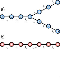
Figure 1: (Color online) (a) Ten site Y spin chain network. Its equivalent one-dimensional representation is shown in (b).

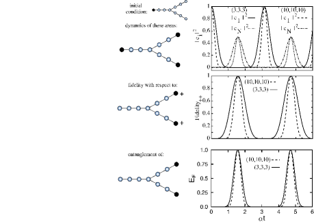
Figure 2: (Color online) Results of simulations on a (3,3,3) and a (10,10,10) Y spin chain system, with nearest neighbour couplings chosen to satisfy (2) and the hub branching rule. Initial condition: $c_{1}=1$ Upper panel: $|c_{1}|^{2}$ and $|c_{N}|^{2}$ with respect to the rescaled time $\alpha t$. Middle panel: corresponding fidelity with respect to the output state $\left|+\right\rangle$. Lower panel: entanglement of formation of chain ends state.

Note that maximally entangled states can also be produced if the length of the output branches is different from the length of the input branch, as long as the couplings satisfy (2) and the hub branching rule. Indeed, in the limit the length of the input branch can be reduced to zero, so the excitation is effectively made at the centre of an odd $N$ chain. This limit may be helpful for some physical realizations, although having an actual input branch may be more practical in some cases.

We can quantify the entanglement at the output using the entanglement of formation, $E_{F}$, which measures the number of Bell states required to create the state of interest. For a two qubit state it is given by: $E_{F}({\rho})=h\left(\frac{1+\sqrt{1-\tau}}{2}\right)$ where $h(x)=-x\log_{2}(x)-(1-x)\log_{2}(1-x)$ is the Shannon entropy function. $\tau$ is the “tangle” or “concurrence” squared: $\tau={\cal C}^{2}=\left[\max\{\lambda_{1}-\lambda_{2}-\lambda_{3}-\lambda_{4},0\}\right]^{2}$. The $\lambda$’s are the square roots of the eigenvalues, in decreasing order, of the matrix ${\rho}\tilde{{\rho}}={\rho}\;\sigma_{y}^{A}\otimes\sigma_{y}^{B}{\rho}^{*}\sigma_{y}^{A}\otimes\sigma_{y}^{B}$, where ${\rho}^{*}$ denotes the complex conjugation of ${\rho}$ in the computational basis $\left|00\right\rangle,\left|01\right\rangle,\left|10\right\rangle,\left|11\right\rangle$ munro01 . $E_{F}$ between qubits $n_{2}=7$ and $n_{3}=10$ of the (3, 3, 3) structure, and $n_{2}=21$ and $n_{3}=31$ of the (10, 10, 10) structure are shown in the lower panel of Fig. 2, as a function of time following initialization of the excitation on site 1. As expected, a maximally entangled state is obtained after a time $\pi/2\alpha$ and at intervals of $\pi/\alpha$ thereafter.

To provide a resource, having generated and distributed entanglement using a spin chain system, it should be isolated or frozen in some way. Clearly, as illustrated in Fig. 2, the arrival time at the output relative to the preparation time at the input is known. At this point, particularly if a number of such states are to be purified before use, the dynamics have to be halted. This could be done by extracting an entangled state (e.g. with swap operations) from the spin chain system and transferring it to a storage system of qubits, or to members of spatially separated quantum registers or processors. (see e.g. spi06 ). Another possibility is to physically isolate the two nodes at the end of the chain, after the entanglement has formed there. If fast local control of the couplings is possible, then the state could indeed be frozen at the ends of the output branches. To achieve this the couplings have to be switched, fast on a timescale set by the chain dynamics illustrated in Fig. 2, simultaneously on both output branches. Both of these methods present obvious difficulties, and are rather cumbersome, so we now discuss a new approach to freezing separated entanglement, which could be very effective for some realizations of the spin chain systems.

A very simple action that can be taken at the end-chain entanglement arrival time is to apply a phase flip to just one of the two output spins, transforming the state to $\left|-\right\rangle$. For extended chains this is not an eigenstate. However, from the symmetry of the Hamiltonian, its subsequent dynamics cannot involve the hub or the input branch, so the subsequent ‘revival time’ of the state $\left|-\right\rangle$ at the output is reduced. This in itself might be useful, but if the structure is modified slightly, coordinated action can provide complete freezing.

The required device has a Y structure, with the ultimate spin at each output branch replaced by a bifurcation into two final spins. These both couple to the penultimate spin with a strength reduced by $1/\sqrt{2}$, compared to the single coupling that they replace. In terms of the four end spins of the full device, the natural dynamics will generate a state of the form $\left|\psi_{s}\right\rangle=\frac{1}{2}(\left|0,0,0,1\right\rangle+\left|0,0,1,0\right\rangle+\left|0,1,0,0\right\rangle+\left|1,0,0,0\right\rangle)$. The structure and dynamics are shown in Fig. 3, where we plot the branch end spin probabilities $|c_{n_{i}}|^{2}$ as a function of rescaled time $\alpha t$. If at a probability peak a phase flip is applied to one spin out of each pair, a state of the form $\left|\psi_{a}\right\rangle=\frac{1}{2}(\left|0,0,0,1\right\rangle-\left|0,0,1,0\right\rangle+\left|0,1,0,0\right\rangle-\left|1,0,0,0\right\rangle)$ results. This is an eigenstate of the system and the entanglement is thus frozen. Although four spins are involved, the spatial separation is between two pairs of spins. Each pair can be viewed as a storage buffer for one qubit. The system contains spatially separated and stored bipartite entanglement, which could be released for future use by single qubit operations and/or coupling to other systems at the branch ends.

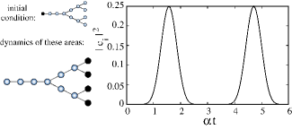
Figure 3: (Color online) Dynamics of $|c_{n_{i}}|^{2}$ (for the output branch end spins) versus the rescaled time $\alpha t$, for the bifurcation structure shown. This follows the initialization condition $c_{1}=1$.

To further quantify the entanglement freezing, we investigate the dependence on the timing of the coordinated phase flips. The upper panel of Fig. 4 shows the fidelity of the state as a function of time, measured against the desired frozen state $\left|\psi_{a}\right\rangle$, for five different choices of the (simultaneous) phase flip timing. This shows that even if the timing is not perfect a high proportion of the state is frozen. The middle panel shows the subsequent dynamics of the remains of the state, for the same five examples of phase flip timing, through plots of the fidelity against the un-flipped state $\left|\psi_{s}\right\rangle$. These amplitudes continue to propagate periodically through the spin chain system, with an overall normalization set by the timing of the phase flips. The lower panel quantifies the amount of bipartite entanglement frozen, showing the entanglement of formation $E_{F}$ as a function of the times $t_{1}$ and $t_{2}$ of each pulse. The encoded basis used for these calculations uses states of the pairs of spins at each chain end and takes the following form: $\left|0_{L}\right\rangle\equiv\left|00\right\rangle$ and $\left|1_{L}\right\rangle\equiv 2^{-1/2}(\left|01\right\rangle-\left|10\right\rangle)$. Clearly if the phase flips are fast compared to the system dynamics, and can be timed sufficiently accurately and simultaneously compared to the period of these dynamics, it is possible to freeze a high quality spatially separated Bell state, encoded in the two pairs of spins.

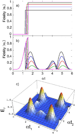
Figure 4: (Color online) Behaviour of the frozen entanglement as a function of phase flip timing, for the system of Fig. 3. (a) Time dependence of the fidelity against $\left|\psi_{a}\right\rangle$ for five different flip times, assumed to be simultaneous with each other. (b) Time dependence of the fidelity against $\left|\psi_{s}\right\rangle$ for the same five flip times. (c) Frozen bipartite entanglement of formation $E_{F}$ as a function of the times $t_{1}$ and $t_{2}$ at which the phase flips are applied.

To conclude, we have shown how entanglement—created and distributed in branching spin chain systems—can be frozen, encoded into pairs of spins located at the ends of Y networks. Such distributed entanglement provides a useful resource, for example for teleportation or distributed quantum processing. In contrast to the use of spin chains to propagate quantum states from one place to another with as high a fidelity as possible, we see some advantage in building up a high fidelity entangled resource off line. Real systems, with their inevitable imperfections, will almost certainly degrade transmission fidelities, even if in principle these approach unity. Certainly, with the ‘off-line’ resource approach, purification pur96 could be applied to build up a higher fidelity resource than can be achieved by direct transmission. This can then be used to transfer quantum states or some form of quantum communication. In effect, the concept of a quantum repeater repeater98 could be employed in a solid state, spin chain scenario. The key ingredient—entanglement distribution and freezing—results from the basic dynamics of the branched spin chain systems, simply prepared initial states and coordinated single qubit operations. This opens new possibilities for quantum communication in solid state systems, especially as fabrication or creation of solid state systems that can operate as spin chains continues to progress.

B. W. L. acknowledges support from the Royal Society and QIPIRC (No. GR/S82176/01).

References

- (1) C. H. Bennett, et al., Phys. Rev. Lett. 76, 722 (1996).
- (2) H.-J. Briegel, et al., Phys. Rev. Lett. 81, 5932 (1998).
- (3) R. Raussendorf and H. J. Briegel, Phys. Rev. Lett. 86, 5188 (2001).
- (4) S. Bose, Phys. Rev. Lett. 91, 207901 (2003).
- (5) T. J. Osborne and N. Linden, Phys. Rev. A 69, 052315 (2004).
- (6) M. Christandl, et al., Phys. Rev. Lett. 92, 187902 (2004); G. De Chiara, et al., Phys. Rev. A 72 012323 (2005).M.-H. Yung and S. Bose, Phys. Rev. A 71 032310 (2005); P. Karbach and J. Stolze, Phys. Rev. A 72, 030301(R) (2005).
- (7) M. Christandl, et al., Phys. Rev. A 71, 032312 (2005).
- (8) D. Burgarth and S. Bose, Phys. Rev. A 71, 052315 (2005); D. Burgarth and S. Bose, New J. Phys 7, 135 (2005).
- (9) A. Wójcik, et al., Phys. Rev. A 72, 034303 (2005).
- (10) I. D’Amico in Focus on Semiconductor Research (edited by Nova Science Publishers, 2006), (Preprint cond-mat/0511470).
- (11) T. P. Spiller, I. D’Amico and B. W. Lovett, New J. Phys. 9, 20 (2007).
- (12) M. B. Plenio and F.L. Semiao, New J. Phys. 6, 36 (2005); M. J. Hartmann, M. E. Reuter and M. B. Plenio, New J. Phys. 8, 94 (2005).
- (13) M. Avellino, A. J. Fisher and S. Bose, Phys. Rev. A 74, 012321 (2006).
- (14) A. D. Greentree, S. J. Devitt and L. C. L. Hollenberg, Phys. Rev. A 73, 032319 (2006); T. Ohshima, et al., Preprint quant-ph/0702019.
- (15) M. B. Plenio, J. Hartley and J. Eisert, New J. Phys. 7, 73 (2004).
- (16) A. Perales and M. B. Plenio, J. Opt. B 7, S601 (2005).
- (17) S. Yang, Z. Song and C. P. Sun, Eur. Phys. J. B 52, 377 (2006); S. Yang, Z. Song and C. P. Sun, Front. Phys. China 1, 1 (2007).
- (18) S. J. Devitt, A. D. Greentree and L. C. L. Hollenberg, Preprint quant-ph/0511084.
- (19) M. Paternostro, H. McAneney and M. S. Kim, Phys. Rev. Lett. 94, 070501 (2005).
- (20) For our calculations we adopt the fidelity definition of M. A. Nielsen and I. L. Chuang, Quantum Computation and Quantum Information p. 409 (Cambridge University Press 2000).
- (21) W. J. Munro, et al., Phys. Rev. A 64, 030302 (2001).