Measurement of $B\rightarrow D_{s}K\pi$ branching ratios

Abstract

We report a measurement of the exclusive $B^{+}$ meson decay to the final state $D_{s}^{-}K^{+}\pi^{+}$ using $520\times 10^{6}B\bar{B}$ pairs collected near the $\Upsilon(4S)$ resonance, with the Belle detector at the KEKB asymmetric-energy $e^{+}e^{-}$ collider. Using the $D_{S}^{-}\to\phi\pi^{-}$ decay mode to reconstruct $D_{s}^{-}$ mesons, we obtain the branching fraction ${\cal B}(B^{+}\to D_{s}^{-}K^{+}\pi^{+})=(1.77^{+0.12}_{-0.12}{\mathrm{(}stat)}\pm 0.16{\mathrm{(}syst)}\pm 0.23{\cal(B)})\times 10^{-4}$. We also present preliminary results of a study of the two-body $D_{s}K$, $D_{s}\pi$ and $K\pi$ subsystems observed in this final state.

I Introduction

We search for the exclusive decays of charged $B$ mesons into $D_{s}K\pi$ final states. These modes offer rich possibilities for studies of different two-body subsystems, such as $D_{s}K$. For the first decay mode studied, $B^{+}\to D_{s}^{-}K^{+}\pi^{+}$ FOOT , the dominant process is described by the Feynman diagram shown in Fig. 1. This process is mediated by the $b\to c$ quark transition and includes the production of an $s\bar{s}$ pair via a radiative gluon. The $D_{s}K\pi$ final state can also be a result of the $b\to c\to s$ decay chain, where the $D_{s}$ meson and the charged pions are produced in two $W$ boson decays. The Feynman diagram in Fig. 2 describes the dominant process responsible for the second decay mode, $B^{+}\to D_{s}^{+}\bar{D^{0}}$ with $\bar{D^{0}}\to K^{+}\pi^{-}$. Note that the two different processes lead to a similar three-body final state, but with opposite charges for the $D_{s}$ and $\pi$ mesons. We measure the branching fraction of the first decay mode and study two-body subsystems, while the second decay mode is a control channel to check the reliability of the method.

In the following the Belle detector and the data sample are briefly described. Next we discuss the reconstruction of the $D_{s}K\pi$ final states. Finally the determination of the branching fractions together with a preliminary study of the $D_{s}K\pi$ subsystems including $D_{s}K$, $D_{s}\pi$ and $K\pi$ are presented.

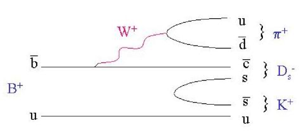
Figure 1: Diagram for the decay $B^{+}\to D_{s}^{-}K^{+}\pi^{+}$.

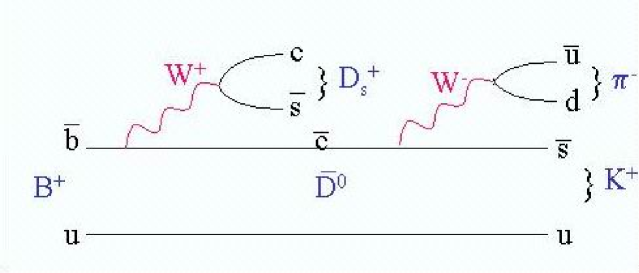
Figure 2: Diagram for the decay $B^{+}\to D_{s}^{+}\bar{D^{0}},\bar{D^{0}}\to K^{+}\pi^{-}$.

II Detector and data Sample

The results are based on a data sample that contains $(520.2\pm 6.8)\times 10^{6}B\bar{B}$ pairs, corresponding to an integrated luminosity of 479 fb^-1, collected with the Belle detector at the KEKB asymmetric-energy $e^{+}e^{-}$ (3.5 on 8 GeV) collider KEKB . KEKB operates at the $\Upsilon(4S)$ resonance ($\sqrt{s}=10.58$ GeV) with a peak luminosity that exceeds $1.7\times 10^{34}~{}{\rm cm}^{-2}{\rm s}^{-1}$. The $\Upsilon(4S)$ resonance is produced with a Lorentz boost of $\beta\gamma=0.425$ nearly along the electron beamline ($z$-axis). The production rates of $B^{+}B^{-}$ and $B^{0}\overline{B}{}^{0}$ pairs are assumed to be equal.

The Belle detector is a large-solid-angle magnetic spectrometer that consists of silicon vertex detector (SVD), a 50-layer central drift chamber (CDC), an array of aerogel threshold Čerenkov counters (ACC), a barrel-like arrangement of time-of-flight scintillation counters (TOF), and an electromagnetic calorimeter composed of CsI(Tl) crystals (ECL) located inside a super-conducting solenoid coil that provides a 1.5 T magnetic field. An iron flux-return located outside of the coil is instrumented to detect $K_{L}^{0}$ mesons and to identify muons (KLM). The detector is described in detail elsewhere BELLE . Two inner detector configurations were used. A 2.0 cm beampipe and a 3-layer silicon vertex detector was used for the first sample of $152\times 10^{6}B\bar{B}$ pairs, while a 1.5 cm beampipe, a 4-layer silicon detector and a small-cell inner drift chamber were used to record the remaining $368\times 10^{6}B\bar{B}$ pairs SVD .

III Reconstruction of $B^{+}\rightarrow D_{s}^{-}K^{+}\pi^{+}$ and $B^{+}\to D_{s}^{+}\bar{D^{0}}$

The reconstruction of $B^{+}\to D_{s}^{-}K^{+}\pi^{+}$ and $B^{+}\to D_{s}^{+}\bar{D^{0}}$ decays consists of the following steps: selection of charged tracks, discrimination between $B\bar{B}$ and continuum events, particle identification and reconstruction of all intermediate decays in $B\rightarrow D_{s}K\pi$ processes. Each of these steps is briefly described below.

III.1 Track selection

Charged tracks with $dr<$ 0.5 cm and $dz<$ 5 cm are selected, where $dr$ and $dz$ are impact parameters measured in the $r$-$\phi$ (transverse) plane and $z$ direction, respectively. Charged tracks are also required to have transverse momenta greater than $100~{}{\rm MeV}/c$.

III.2 Suppression of continuum events

We exploit the event topology to discriminate between spherical $B\bar{B}$ events and the dominant background from jet-like continuum events, $e^{+}e^{-}\rightarrow q\bar{q}$ ($q$ = $u$, $d$, $s$, $c$). We combine event shape variables using all particles in an event to calculate Fox-Wolfram moments FOX and define the $R_{2}$, ratio of second and zeroth moments, as

$$R_{2}=\frac{\sum_{i,j}|\vec{p}_{i}||\vec{p}_{j}|P_{2}(\cos\theta_{ij})}{\sum_{i,j}|\vec{p}_{i}||\vec{p}_{j}|}\,,$$

where $\vec{p}$ indicates the particle momentum, $P_{2}$ is the Legendre polynomial of second order, and $i$, $j$ enumerate all particles in the event. We require $R_{2}$ to be less than 0.4.

III.3 Particle identification

Hadron identification is based on information provided by the CDC, ACC and TOF. For kaons we require ${\cal L}_{K/\pi}>0.6$ and ${\cal L}_{p/K}<0.95$ (veto), where ${\cal L}_{x/y}=\frac{{\cal L}_{x}}{{\cal L}_{x}+{\cal L}_{y}}$ ($x$, $y$ = $\pi$, $K$, $p$) denotes the corresponding likelihood ratio. Pions are selected as non-kaons, satisfying veto conditions for $K$ and $p$: ${\cal L}_{p/K}<0.95$ and ${\cal L}_{K/\pi}<0.95$. In addition, we reject tracks that are consistent with an electron hypothesis. A selection imposed on this ratio results in a typical kaon (pion) identification efficiency ranging from 92% to 97% (94% to 98%) for various decay modes, while 2% to 15% (4% to 8%) of kaon (pion) candidates are misidentified pions (kaons).

III.4 Reconstruction of exclusive $D_{s}^{+}$ decays

The $D_{s}^{+}$ candidates are reconstructed in two final states: $\phi(\to K^{+}K^{-})\pi^{+}$ and $\bar{K^{*}}(892)^{0}(\to K^{-}\pi^{+})K^{+}$. We reconstruct $\phi$ mesons in the $K^{+}K^{-}$ final state. The $\phi$ mass is estimated to be ($1019.70\pm 0.153$) MeV/$c^{2}$, in agreement with the world average value $m_{WA}(\phi)=(1019.460\pm 0.019$) MeV/$c^{2}$  PDG . We accept $K^{+}K^{-}$ pairs satisfying the requirement $\left|m(K^{+}K^{-})-m_{WA}(\phi)\right|<10$ MeV/$c^{2}$. Similarly, the $K^{+}\pi^{-}$ mass spectrum exhibits a $K^{*}(892)^{0}$ signal at a mass of ($892.19\pm 1.80$) MeV/$c^{2}$ ($m_{WA}(K^{*0})=(896.00\pm 0.25$) MeV/$c^{2}$  PDG ); $K^{*0}$ candidates are thus selected with the requirement: $\left|m(K^{+}\pi^{-})-m_{WA}(K^{*0})\right|<100$ MeV/$c^{2}$.

A clear $D_{s}$ meson signal is observed in both channels considered (Figs. 4–4). The fitting procedure – described in the next section – is used to obtain the mean values of the $D_{s}$ mass in each channel. This mass, averaged over two decay channels studied, is estimated to be ($1968.1\pm 0.20{\mathrm{(}stat)}$) MeV/$c^{2}$, which is consistent with the world average value $m_{WA}(D_{s})=(1968.2\pm 0.5)$ MeV/$c^{2}$  PDG . The invariant mass of $D_{s}$ candidates is required to satisfy the criterion $\left|m(D_{s})-m_{WA}(D_{s})\right|<15$ MeV/$c^{2}$, corresponding to a window of approximately three standard deviations about the $D_{s}$ mass.

III.5 Reconstruction of $B$ mesons

$B$ mesons are reconstructed combining $D_{s}$ candidates with identified kaons and pions. In exclusive reconstruction of $B$ mesons two kinematic variables are used: the energy difference, $\Delta E$, and the beam-energy-constrained mass, $M_{\mathrm{bc}}$. These are defined as:

$$\Delta E=E_{B}-E_{\mathrm{beam}}$$ (1)

and

$$M_{\mathrm{bc}}=\sqrt{E_{\mathrm{beam}}^{2}-p_{B}^{2}}\,,$$ (2)

where $E_{B}$ and $P_{B}$ are the reconstructed energy and momentum of the $B$ candidate, and $E_{\mathrm{beam}}$ is the run-dependent beam energy, all expressed in the centre-of-mass (CM) frame. We use the dedicated Monte Carlo (MC) sample of $B\rightarrow D_{s}K\pi$ decays to define signal regions in $\Delta E$ and $M_{\mathrm{bc}}$ as $|\Delta E|<0.03$ GeV and $M_{\mathrm{bc}}>5.27$ GeV/$c^{2}$. For all $B$ candidates, a loose requirement on the goodness of the $D_{s}K\pi$ vertex fit – with the $D_{s}$ mass constrained to the world average value – is also applied ($\chi^{2}_{B}<50$).

From MC simulation we determine that the background contribution from $B^{+}\to((c\bar{c})\to K^{+}K^{-}\pi^{+}\pi^{-})K^{+}$ decays, where $(c\bar{c})$ are charmonium states such as the $J/\psi$ or $\eta_{c}$, is removed by discarding all events that satisfy the requirement: 2.88 GeV/$c^{2}<M(K^{+}K^{-}\pi^{+}\pi^{-})<$ 3.18 GeV/$c^{2}$.

For $B^{+}\rightarrow D_{s}^{+}\bar{D^{0}}$ candidate events a requirement on $K^{+}\pi^{-}$ invariant mass is imposed: $|m(K^{+}\pi^{-})-m_{WA}(D^{0})|<0.015$ GeV/$c^{2}$ PDG . This condition is determined by using $D_{s}^{+}K^{+}\pi^{-}$ combinations for events from the ($\Delta E,M_{\mathrm{bc}}$) signal region and plotting the invariant mass of $K^{+}\pi^{-}$ pairs as shown in Fig. 5.

After selection requirements, 8.8%(10.6%) of events with reconstructed $D_{s}\to\phi\pi$ ($D_{s}\to K^{*0}K$) decays have more than one $B$ candidate. In these cases we select the $B$ candidate having the smallest value of $\chi_{B}^{2}$. If there are two or more combinations with the same value of $\chi^{2}_{B}$, the one containing a kaon – originating directly from the $B$ decay – with the highest likelihood ratio ${\cal L}_{K/\pi}$ is selected.

For events passing all selection criteria mentioned above the $\Delta E$ distributions (requiring $M_{\mathrm{bc}}>5.27$ GeV/c²) and $M_{\mathrm{bc}}$ distributions (requiring $|\Delta E|<0.03$ GeV) are examined. The plots shown in Figs. 6–9 exhibit clear signals from the corresponding $B$ meson decays. In addition, an excess of events can be seen in the range $\Delta E\in(-0.2,-0.08)$ GeV, probably due to events with one unreconstructed particle, such as a $\pi^{0}$ or $\gamma$, in the final state.

IV Determination of $B\rightarrow D_{s}K\pi$ branching fraction

The branching fractions are calculated using the formula:

$${\cal B}(B\rightarrow D_{s}K\pi)=\frac{N_{S}/\varepsilon}{N_{B\bar{B}}\cdot{\cal B}_{int}}$$ (3)

where $N_{B\bar{B}}$ is the number of produced $B\bar{B}$ pairs, $N_{S}$ is the number of reconstructed $B\rightarrow D_{s}K\pi$ events, $\varepsilon$ denotes the reconstruction efficiency and ${\cal B}_{int}$ is the product of branching fractions of intermediate resonances, present in the respective $B\rightarrow D_{s}K\pi$ processes (values summarised in Table 1 are taken from the Ref. PDG ).

Table 1: Branching fractions of intermediate resonances present in $B^{+}\rightarrow D_{s}^{-}K^{+}\pi^{+}$ and $B^{+}\rightarrow D_{s}^{+}\bar{D^{0}}$ decays (from the PDG).

Decay	Branching fraction [%]
$D_{s}^{+}\rightarrow\phi\pi^{+},\;\;\phi\rightarrow K^{+}K^{-}$	2.16 $\pm$ 0.28
$D_{s}^{+}\rightarrow\bar{K^{*}}(892)^{0}K^{+},\;\;\bar{K^{*}}(892)^{0}\rightarrow K^{-}\pi^{+}$	2.5 $\pm$ 0.5
$D^{0}\rightarrow K^{-}\pi^{+}$	3.80 $\pm$ 0.07

IV.1 Determination of the number of $B\rightarrow D_{s}K\pi$ events

The yields of $B\rightarrow D_{s}K\pi$ events are determined from an unbinned extended maximum likelihood fit to $(\Delta E,M_{\mathrm{bc}},m_{D_{S}})$ distributions using the MINUIT MINUIT package. The likelihood function is given by:

$${\cal L}(\vec{\theta})=\prod_{i=1}^{N}f(\vec{x}_{i}|\vec{\theta})\,,$$

where $\vec{x}_{i}$ is a vector of independently measured values of the probability density function $f(\vec{x}|\vec{\theta})$. The index $i$ ($i$ = 1, 2, $\ldots$, $N$) counts the number of reconstructed events used in the fit. The vector $\vec{\theta}=(\theta_{1},\ldots,\theta_{n})$ contains the parameters that are obtained by maximizing the likelihood function:

$$\hat{\vec{\theta}}=\max_{\vec{\theta}}{\cal L}(\vec{\theta})$$

The probability density function $f$ contains a Poisson factor to include the relation between the estimated number of all events ($N_{S}+N_{B}$) and the number of reconstructed events $N$, and is defined as:

$$f(\vec{x}|\vec{\theta})={g(\vec{x}|\vec{\theta})}\cdot\frac{1}{N!}(N_{S}+N_{B})^{N}e^{-N_{S}-N_{B}}\,,$$

while

$$g(\vec{x}|\vec{\theta}) =\frac{N_{S}}{N_{S}+N_{B}}\cdot\frac{1}{\sigma_{\Delta E}\sqrt{2\pi}}\exp\biggl{[}-\frac{\Delta E^{2}}{2{\sigma_{\Delta E}}^{2}}\biggr{]}\cdot$$ (a)

$$\qquad\qquad\frac{1}{\sigma_{M_{\mathrm{bc}}}\sqrt{2\pi}}\exp\biggl{[}-\frac{\left(M_{\mathrm{bc}}-m_{WA}(B)\right)^{2}}{2{\sigma_{M_{\mathrm{bc}}}}^{2}}\biggr{]}\cdot$$ (b)

$$\frac{1}{\sqrt{2\pi}}\left(\frac{1}{\sigma_{m_{D_{S}1}}}\exp\biggl{[}-\frac{\left(m_{D_{S}}-m_{WA}(D_{s})\right)^{2}}{2{\sigma_{m_{D_{S}1}}}^{2}}\biggr{]}+\frac{1}{\sigma_{m_{D_{S}2}}}\exp\biggl{[}-\frac{\left(m_{D_{S}}-m_{WA}(D_{s})\right)^{2}}{2{\sigma_{m_{D_{S}2}}}^{2}}\biggr{]}\right)$$ (c)

$$+\frac{N_{B}}{N_{S}+N_{B}}\cdot\frac{1}{\mathcal{N}}\left(w_{0}+w_{1}\Delta E+w_{2}{\Delta E}^{2}\right)\cdot$$ (d)

$$\qquad\frac{M_{\mathrm{bc}}}{\sqrt{s}/2}\cdot\sqrt{1-\left(\frac{M_{\mathrm{bc}}}{\sqrt{s}/2}\right)^{2}}\exp\left\{arg\biggl{[}1-\left(\frac{M_{\mathrm{bc}}}{\sqrt{s}/2}\right)^{2}\biggr{]}\right\}$$ (e)

$$\qquad\left(p_{0}+p_{1}m_{D_{S}}+p_{2}{m_{D_{S}}}^{2}\right)\,.$$ (f)

The first three contributions in this formula ((a),(b) and (c)) describe the signal parameterized by four Gaussian functions: one for $\Delta E$, one for $M_{\mathrm{bc}}$ and two Gaussians with the same mean and different widths for the ${m_{D_{S}}}$ distributions. The last three terms describe the background: second-order polynomials for $\Delta E$ and ${m_{D_{S}}}$ variables ((d) and (f)), and the so-called ARGUS function ARGUS in (e) for the $M_{\mathrm{bc}}$ variable.

In this notation $\vec{x}=(\Delta E,M_{\mathrm{bc}},m_{D_{S}})$ and $\vec{\theta}=(N_{S},N_{B},w_{0},w_{1},w_{2},p_{0},p_{1},p_{2},arg,\sigma_{\Delta E},\\ \sigma_{M_{\mathrm{bc}}},\sigma_{m_{D_{S}1}},\sigma_{m_{D_{S}2}}$). Here $N_{S}$ and

Table 2: Values of the $M_{\mathrm{bc}}$, $\Delta E$ and $m_{D_{S}}$ parameters, as extracted from the fits described in the text.

Decay	$M_{bc}$ [MeV/c2]	$\Delta E$ [MeV]	$m_{D_{S}}$ [MeV/c2]
$B^{+}\rightarrow D_{s}^{-}(\to\phi\pi^{-})K^{+}\pi^{+}$	$5279.4\pm 0.2$	$-1.3\pm 0.7$	$1967.8\pm 0.3$
$B^{+}\rightarrow D_{s}^{-}(\to K^{*}(892)^{0}K^{-})K^{+}\pi^{+}$	$5279.2\pm 0.2$	$-2.1\pm 0.9$	$1968.7\pm 0.4$
$B^{+}\rightarrow D_{s}^{+}(\to\phi\pi^{+})\bar{D^{0}}$	$5279.2\pm 0.1$	$-0.3\pm 0.5$	$1968.2\pm 0.2$
$B^{+}\rightarrow D_{s}^{+}(\to\bar{K^{*}}(892)^{0}K^{+})\bar{D^{0}}$	$5279.1\pm 0.1$	$-0.2\pm 0.6$	$1967.9\pm 0.2$

$N_{B}$ denote the number of signal events and the number of background events, respectively, while $w_{0},w_{1},w_{2},p_{0},p_{1},p_{2}$ are the parameters of the polynomials, $arg$ is a parameter of the ARGUS function and $\sigma_{\Delta E}$, $\sigma_{M_{\mathrm{bc}}}$, $\sigma_{m_{D_{S}1}}$, $\sigma_{m_{D_{S}2}}$ are the respective widths of the Gaussian functions. The factor $\mathcal{N}$ provides a normalization.

When performing the fit, all $\vec{\theta}$ parameters are allowed to float. The mean values of $\Delta E$, $M_{\mathrm{bc}}$ and $m_{D_{S}}$ obtained from the fit are collected in Table 2. The quoted $M_{\mathrm{bc}}$ ($m_{D_{S}}$) values are mutually consistent and also in agreement with the world average value $m_{WA}(B)$ ($m_{WA}(D_{S})$) PDG .

The determination of the number of reconstructed decays ($N$) proceeds in two steps:

• The fit to the ($\Delta E$, ${M_{\mathrm{bc}}}$, $m_{D_{S}}$) distribution is evaluated in the signal region (with requirements on all intermediate resonances), resulting in $N_{0}$ events.

• For decays containing $K^{*}(892)^{0}$ meson, a fit to the sample of events from the $K^{*}(892)^{0}$ mass sidebands ([0.746,0.796] GeV/$c^{2}$ and [0.996,1.046] GeV/$c^{2}$) is also performed. It yields the number of background events, $N_{1}$, peaking in the signal region and therefore contributing to the $N_{0}$ value. The same procedure is applied also for the efficiency calculation. This step is motivated by a MC study, where such a background contribution was found. The study also revealed that for the $D_{s}\to\phi\pi$ decay mode this background contribution is negligible.

Finally, the number of $B\rightarrow D_{s}K\pi$ events is calculated as:

$$N=N_{0}-N_{1}.$$ (4)

The values of $N_{0}$, $N_{1}$ and $N$ for the analysed decays are listed in Table 3.

Table 3: Numbers of the signal and background events for analysed decays and efficiencies of their reconstructions. The errors are statistical only.

Decay	$N_{0}$	$N_{1}$	$N$	$\varepsilon$ [%]
$B^{+}\rightarrow D_{s}^{-}(\phi\pi)K^{+}\pi^{+}$	$276.5\;^{+19.3}_{-18.6}$	-	$276.5\;^{+19.3}_{-18.6}$	$13.89\pm 0.13$
$B^{+}\rightarrow D_{s}^{-}(K^{\star 0}K^{-})K^{+}\pi^{+}$	$299.5\;^{+26.0}_{-25.1}$	$48.2\;^{+18.6}_{-13.7}$	$251.3\;^{+32.0}_{-28.6}$	$9.05\pm 0.11$
$B^{+}\rightarrow D_{s}^{+}(\phi\pi)\bar{D^{0}}$	$512.3\;^{+23.4}_{-22.8}$	-	$512.3\;^{+23.4}_{-22.8}$	$14.09\pm 0.13$
$B^{+}\rightarrow D_{s}^{+}(\bar{K}^{\star 0}K^{+})\bar{D^{0}}$	$508.0\;^{+24.1}_{-23.4}$	$47.8\;^{+10.4}_{-7.6}$	$460.2\;^{+26.2}_{-24.6}$	$10.03\pm 0.12$

Table 4: Values of contributions (in %) to the overall systematic uncertainty in the branching fraction for the $B^{+}\rightarrow D_{s}^{-}K^{+}\pi^{+}$ decay.

Individual	Values [%] for studied decays:
contribution	$B^{+}\rightarrow D_{s}^{-}(\phi\pi^{-})K^{+}\pi^{+}$	$B^{+}\rightarrow D_{s}^{-}(K^{\star 0}K^{-})K^{+}\pi^{+}$
$\Delta{\cal B}^{\varepsilon}$	5.05	4.16
$\Delta{\cal B}^{rng}$	1.26	2.39
$\Delta{\cal B}^{\Gamma}$	1.57	8.04
$\Delta{\cal B}^{sel}$	2.43	0.72
$\Delta{\cal B}^{id}$	5	5
$\Delta{\cal B}^{trck}$	5	5
$\Delta{\cal B}^{B\bar{B}}$	1.3	1.3
total	9.34	11.83

IV.2 Determination of the reconstruction efficiency

The reconstruction efficiency ($\varepsilon$) of each channel in question is determined using MC samples of $10^{5}$ $e^{+}e^{-}\rightarrow\Upsilon(4S)\rightarrow B^{+}B^{-}$ decays. These samples are generated in two subsets corresponding to the two inner detector configurations that were used in Belle experiment (denoted as SVD1 and SVD2). Each subset contains $5\times 10^{4}$ events. In each event, one of the charged $B$ mesons decays to the appropriate $D_{s}^{\mp}K^{\pm}\pi^{\pm}$ ($D_{s}^{+}\bar{D^{0}}$/$D_{s}^{-}D^{0}$) final state. These dedicated MC samples are subjected to the same analysis as the data, yielding the number of reconstructed events, $N_{MC_{1}}$ and $N_{MC_{2}}$, which corresponds to the SVD1 and SVD2 samples, respectively. These values divided by the number of all simulated events, gives partial reconstruction efficiencies for the studied decays:

$$\varepsilon_{1}=\frac{N_{MC_{1}}}{50000},\qquad\varepsilon_{2}=\frac{N_{MC_{2}}}{50000}$$

The final efficiences for all studied decays are obtained by calculating the weighted averages of the values defined above:

$$\varepsilon=\frac{N_{B\bar{B}1}\cdot\varepsilon_{1}+N_{B\bar{B}2}\cdot\varepsilon_{2}}{N_{B\bar{B}1}+N_{B\bar{B}2}}$$

where $N_{B\bar{B}1}$ and $N_{B\bar{B}2}$ are the numbers of $B\bar{B}$ events collected during the SVD1 and SVD2 running periods, respectively. Values of efficiencies for studied decays are presented in Table 3.

IV.3 Studies of systematic uncertainties

The following sources of systematic uncertainties are taken into account (cf. Table 4):

• $\Delta{\cal B}^{\varepsilon}$ - uncertainty of efficiency determination estimated as a statistical error of its measurement, i.e.

  $$\Delta\varepsilon=\sqrt{\left(\frac{N_{B\bar{B}1}}{N_{B\bar{B}1}+N_{B\bar{B}2}}\right)^{2}\cdot(\Delta\varepsilon_{1})^{2}+\left(\frac{N_{B\bar{B}2}}{N_{B\bar{B}1}+N_{B\bar{B}2}}\right)^{2}\cdot(\Delta\varepsilon_{2})^{2}}$$

  where $\Delta\varepsilon_{1}$ and $\Delta\varepsilon_{2}$ are statistical uncertainities on partial efficiencies.
  Considering the control channel and taking into account a mismatch between branching fractions calculated for the MC sample (cf. IV.D subsection), an additional contribution to the efficiency systematics can be assigned. The shift (with an error) between the obtained branching fraction value and the generator value is calculated and the corresponding systematic error is determined. This factor is summed in quadrature with the above $\Delta\varepsilon$ value to evaluate the final $\Delta{\cal B}^{\varepsilon}$ contribution.

• $\Delta{\cal B}^{sel}$ - uncertainty due to the selection procedure. To estimate this error, the requirement for the $R_{2}$ parameter is varied: $R_{2}<0.40\rightarrow R_{2}<0.35$.

• $\Delta{\cal B}^{rng}$ - error from changing the range of the fit to the $\Delta E$ variable. For $B^{+}\rightarrow D_{s}^{-}K^{+}\pi^{+}$ decays this range is changed from $(-0.08,0.2)$ GeV to $(-0.12,0.2)$ GeV. For each case the number of signal events $N_{0}^{rng}$ is determined, and the deviation from the $N_{0}$ value is calculated.

• $\Delta{\cal B}^{\Gamma}$ - uncertainty in the signal width. The width of the signal peak, as obtained from the fit to the $\Delta E/M_{\mathrm{bc}}$ using MC sample, is then used as a fixed parameter in the same fit to data. The fixing procedure is applied sequentially: for $\Delta E$, for $M_{\mathrm{bc}}$ and for both the $\Delta E$ and $M_{\mathrm{bc}}$ signal peaks. Finally, the maximum deviation from the $N_{0}$ value is chosen.

• $\Delta{\cal B}^{id}$ - uncertainty of particle identification in Belle experiment. A standard value of 1% per charged particle is assumed and uncertainties from kaons and pions are combined linearly, thus giving an overall contribution of 5 %.

• $\Delta{\cal B}^{trck}$ - uncertainty of track reconstruction. A standard value of 1% per charged track is assumed giving an overall contribution of 5 %.

• $\Delta{\cal B}^{B\bar{B}}$ - uncertainty of the number of $B\bar{B}$ mesons used as data sample. Value of 1.3% is assumed in each studied decay.

All contributions are assumed to be independent, hence the overall systematic error is obtained by summing those contributions in quadrature. The last three sources of systematic uncertainties are assumed to be common to all decays studied. All information about systematic uncertainties is collected in Table 4.

Table 5: Branching fraction of studied decays.

studied	${\cal B}$	uncertainties				signif.
decays	$\times 10^{-4}$	stat.(+)	stat.(-)	syst.	${\cal B}_{int}$	[$\sigma$]
$B^{+}\rightarrow D_{s}^{-}(\phi\pi)K^{+}\pi^{+}$	1.77	0.12	0.12	0.16	0.23	27.5
$B^{+}\rightarrow D_{s}^{-}(K^{\star 0}K^{-})K^{+}\pi^{+}$	2.15	0.27	0.24	0.25	0.43	23.1
$B^{+}\rightarrow D_{s}^{+}(\phi\pi)\bar{D^{0}}$	85.17	3.89	3.77	-	11.15	46.4
$B^{+}\rightarrow D_{s}^{+}(K^{\star 0}K^{+})\bar{D^{0}}$	92.89	5.29	4.97	-	18.66	42.1

IV.4 Discussion of the results

The values of branching fraction for the decays $B^{+}\rightarrow D_{s}^{-}K^{+}\pi^{+}$ and $B^{+}\rightarrow D_{s}^{+}\bar{D^{0}}$ are collected in Table 5. Here the ’${\cal B}_{int}$’ error is due to uncertainties in the branching fractions for the decays of intermediate resonances present in the decay in question (Table 1). The significance of the signal (Table 5) is evaluated according to the formula $\sqrt{-2ln({\cal L}_{0}/{\cal L})}$, where ${\cal L}$ is the likelihood calculated for the nominal fit and ${\cal L}_{0}$ is the respective likelihood function for a fit with the number of signal events fixed to zero.

The final results for the branching fractions for the channels studied, according to Table 5, are as follows:

For $D_{s}\to\phi(\to K^{+}K^{-})\pi$ decay modes:

$${\cal B}(B^{+}\to D_{s}^{-}K^{+}\pi^{+})=(1.77^{+0.12}_{-0.12}({\mathrm{s}tat})\pm 0.16({\mathrm{s}yst})\pm 0.23({\mathrm{\cal B}_{int})})\times 10^{-4}~{}~{}$$ (5)

$${\cal B}(B^{+}\to D_{s}^{+}\bar{D^{0}})=(8.52^{+0.39}_{-0.38}({\mathrm{s}tat}))\times 10^{-3}~{}~{}~{}~{}~{}~{}~{}~{}~{}~{}~{}~{}~{}~{}~{}~{}~{}~{}~{}~{}~{}~{}~{}~{}~{}~{}~{}~{}~{}~{}~{}~{}~{}~{}~{}~{}~{}~{}~{}~{}~{}~{}$$ (6)

and for $D_{s}\to\bar{K^{*}}(892)^{0}(\to K^{-}\pi^{+})K$ decay modes:

$${\cal B}(B^{+}\to D_{s}^{-}K^{+}\pi^{+})=(2.15^{+0.27}_{-0.24}({\mathrm{s}tat})\pm 0.25({\mathrm{s}yst})\pm 0.43({\mathrm{\cal B}_{int})})\times 10^{-4}$$ (7)

$${\cal B}(B^{+}\to D_{s}^{+}\bar{D^{0}})=(9.29^{+0.53}_{-0.50}({\mathrm{s}tat}))\times 10^{-3}~{}~{}~{}~{}~{}~{}~{}~{}~{}~{}~{}~{}~{}~{}~{}~{}~{}~{}~{}~{}~{}~{}~{}~{}~{}~{}~{}~{}~{}~{}~{}~{}~{}~{}~{}~{}~{}~{}$$ (8)

The results presented here are compatible with the values reported by the BaBar collaboration BABAR . The branching fraction for the $B^{+}\rightarrow D_{s}^{+}\bar{D^{0}}$ decay is consistent with the world average value given by Particle Data Group (PDG): ${\cal B}_{PDG}(B^{+}\rightarrow D_{s}^{+}\bar{D^{0}}$) = ($1.09\pm 0.27\%$) PDG .

The same study is also performed for a large statistics MC samples simulating the following processes: $e^{+}e^{-}\to B^{+}B^{-},B^{0}\bar{B^{0}}$ and $q\bar{q}$($q=u,d,s,c$). These samples are subjected to the same analysis procedure as data; the signal from the decay $B^{+}\to D_{s}^{+}\bar{D^{0}}$ is fitted as described in subsection IV.A. The resulting branching fractions for the decays $B^{+}\to D_{s}^{+}(\rightarrow\phi\pi^{+})\bar{D^{0}}$ and $B^{+}\to D_{s}^{+}(\rightarrow K^{*0}K^{+})\bar{D^{0}}$ are $(9.28^{+0.23}_{-0.22})\times 10^{-3}$ and $(8.92^{+0.23}_{-0.22})\times 10^{-3}$, respectively. They are compatible with the values assumed in the MC generator: ${\cal B}(B^{+}\to D_{s}^{+}\overline{D^{0}})=9.06\times 10^{-3}$ (Differences within statistical errors of the extracted MC values are used as conservative estimates of systematic uncertainties for the reconstruction efficiencies, as described above.)

IV.5 Studies of two-body subsystems $D_{s}K$, $D_{s}\pi$ and $K\pi$

The study of two-body subsystems in the $D_{s}K\pi$ final states is driven by two facts. The first one is the lack of resonances in the $D^{+}\pi^{-}$ invariant mass above the value of 2.55 GeV/c² observed by Belle BDPIPI , where the respective three-body decay is $B^{+}\to D^{+}\pi^{-}\pi^{-}$. Second, the $D_{s}^{-}\pi^{+}$ and $K^{+}\pi^{+}$ pairs cannot form ’standard’ $q\bar{q}$ resonances, so any signal observed in these subsystems would indicate the presence of some exotic states such as hybrid mesons, tetraquarks, etc.

Below we concentrate on the $D_{s}^{-}K^{+}\pi^{+}$ final state. Figures 10–12 show the Dalitz plots of all possible combinations of invariant-mass squared: $M^{2}(D_{s}K)$, $M^{2}(D_{s}\pi)$ and $M^{2}(K\pi)$. All distributions are shown both for the signal region and the $\Delta E$ sidebands. The structure visible in the invariant mass of the $D_{s}\pi$ subsystem in the mass region around 3 GeV/c² corresponds to the decays $B^{+}\to(c\bar{c})K^{+}$. Preliminary studies of these Dalitz plots do not confirm contributions of any exotic states in the two-body subsystems. However, further studies might reveal some enhancements such as that observed by BaBar in the $m(D_{s}^{-}K^{+})$ spectrum BABAR . Detailed analyses of the two-body subsystems are therefore still in progress.

V Acknowledgments

We thank the KEKB group for the excellent operation of the accelerator, the KEK cryogenics group for the efficient operation of the solenoid, and the KEK computer group and the National Institute of Informatics for valuable computing and Super-SINET network support. We acknowledge support from the Ministry of Education, Culture, Sports, Science, and Technology of Japan and the Japan Society for the Promotion of Science; the Australian Research Council and the Australian Department of Education, Science and Training; the National Science Foundation of China and the Knowledge Innovation Program of the Chinese Academy of Sciences under contract No. 10575109 and IHEP-U-503; the Department of Science and Technology of India; the BK21 program of the Ministry of Education of Korea, the CHEP SRC program and Basic Research program (grant No. R01-2005-000-10089-0) of the Korea Science and Engineering Foundation, and the Pure Basic Research Group program of the Korea Research Foundation; the Polish State Committee for Scientific Research; the Ministry of Education and Science of the Russian Federation and the Russian Federal Agency for Atomic Energy; the Slovenian Research Agency; the Swiss National Science Foundation; the National Science Council and the Ministry of Education of Taiwan; and the U.S. Department of Energy.

Figure 3: Invariant mass distribution for $\phi\pi^{-}$ pairs (points) together with the curve representing the fit result in the range of the $D_{s}^{-}$ meson mass (red dashed line) for $B^{+}\rightarrow D_{s}^{-}K^{+}\pi^{+}$ decay. The signal is parameterized by two Gaussians, while the background is described by a second-order polynomial. The spectrum corresponds to the ($\Delta E,M_{\mathrm{bc}}$) signal box.

Figure 4: Invariant mass distribution for $K^{*}(892)^{0}K^{-}$ pairs (points) together with the curve representing the fit result in the range of the $D_{s}^{-}$ meson mass (red dashed line) for $B^{+}\rightarrow D_{s}^{-}K^{+}\pi^{+}$ decay. The signal is parameterized by two Gaussians, while the background is described by a second-order polynomial. The spectrum corresponds to the ($\Delta E,M_{\mathrm{bc}}$) signal box.

Figure 5: Invariant mass distribution for $K^{+}\pi^{-}$ pairs (points) together with the curve representing the fit result in the range of the $\bar{D}^{0}$ meson for the $B^{+}\rightarrow D_{s}^{+}\bar{D}^{0}$ decay. The signal is parameterized by a single Gaussian, while the background is described by a first-order polynomial. The spectrum corresponds to the ($\Delta E,M_{\mathrm{bc}}$) signal box.

Figure 6: Distributions of the $\Delta E$ (top) and $M_{\mathrm{bc}}$ variables (bottom) for the decay $B^{+}\rightarrow D_{s}^{-}K^{+}\pi^{+}$, $D_{s}^{-}\to\phi\pi^{-}$. Points correspond to data and the dashed (red) line represents results of the fit described in the text.

Figure 7: Distributions of the $\Delta E$ (top) and $M_{\mathrm{bc}}$ variables (bottom) for the decay $B^{+}\rightarrow D_{s}^{-}K^{+}\pi^{+}$, $D_{s}^{-}\to K^{*}(892)^{0}K^{-}$. Points correspond to data and the dashed (red) line represents results of the fit described in the text.

Figure 8: Distributions of the $\Delta E$ (top) and $M_{\mathrm{bc}}$ variables (bottom) for the decay $B^{+}\rightarrow D_{s}^{+}\bar{D^{0}}$, $D_{s}^{+}\to\phi\pi^{+}$. Points correspond to data and the dashed (red) line represents results of the fit described in the text.

Figure 9: Distributions of the $\Delta E$ (top) and $M_{\mathrm{bc}}$ variables (bottom) for the decay $B^{+}\rightarrow D_{s}^{+}\bar{D^{0}}$, $D_{s}^{-}\to\bar{K^{*}}(892)^{0}K^{+}$. Points correspond to data and the dashed (red) line represents results of the fit described in the text.

Figure 10: The Dalitz plots of $M_{D_{s}K}^{2}$ vs $M_{D_{s}\pi}^{2}$ for the signal box (upper plot) and $\Delta E$ sidebands (lower plot).

Figure 11: The Dalitz plots of $M_{D_{s}\pi}^{2}$ vs $M_{K\pi}^{2}$ for the signal box (upper plot) and $\Delta E$ sidebands (lower plot).

Figure 12: The Dalitz plots of $M_{D_{s}K}^{2}$ vs $M_{K\pi}^{2}$ for the signal box (upper plot) and $\Delta E$ sidebands (lower plot).

References

(1)
Throughout this paper, the inclusion of the charge conjugate mode
decay is implied unless otherwise stated.
(2)
S. Kurokawa and E. Kikutani, Nucl. Instr. and. Meth. A 499, 1 (2003),
and other papers included in this volume.
(3)
A. Abashian et al. (Belle Collab.), Nucl. Instr. and Meth. A 479, 117 (2002).
(4)
Z. Natkaniec et al. (Belle SVD2 Group), Nucl. Instr. and Meth. A 560, 1 (2006).
(5)
G. C. Fox and S. Wolfram, Phys. Rev. Lett. 41, 1581 (1978).
(6)
W.-M. Yao et al. (Particle Data Group), J. Phys. G 33, 1 (2006).
(7)
F. James, CERN Program Library Long Writeup D506.
(8)
H. Albrecht et al. (ARGUS Collab.), Phys. Lett. B 241, 278 (1990).
(9)
B. Aubert et al. (BaBar Collab.), arXiv:0707.1043v1 [hep-ex].
(10)
A. Satpathy et al. (Belle Collab.), Phys. Lett. B 553 159 (2003).