General quantum phase estimation and calibration of a timepiece in a quantum dot system

Abstract

We present a physical scheme for implementing quantum phase estimation via weakly coupled double quantum-dot molecules embedded in a microcavity. During the same process of implementation, we can also realize the calibration of timepiece based on the estimated phase. We use the electron-hole pair states in coupled double quantum-dot molecules to encode quantum information, where the requirement that two quantum dots are exactly identical is not necessary. Our idea can also be generalized to other systems, such as atomic, trapped ion and linear optics system.

I introduction

Relative phase plays an important role in quantum information. The encoding of information into the relative phase of quantum systems has been extensively used in quantum cryptographic 1 , quantum cloning 2 , geometric quantum computation 3 and so on. Phase estimation based on discrete quantum Fourier transform (QFT) is a comparatively good method to resolve some phase problems. The phase estimation is a procedure of measuring an certain unknown phase with high precision, which is also the key ingredient for resolving some complex quantum algorithms 4a ; 4b ; 4c , e.g. factoring problem and order-finding problem. Therefore quantum phase estimation is a very important tool in quantum communication and quantum computation.

In order to estimate an unknown phase $\phi$ ($\phi\in(0,2\pi])$, we must use an oracle in the process because the phase estimation procedure is not a complete quantum algorithm in its own right. At the same time, the generation of a state $|u\rangle$ with an eigenvalue $e^{i\phi}$ is necessary. In addition, we should also find a unitary transformation $U$, which satisfies

$$U|u\rangle=\exp({i\phi})|u\rangle.$$

Controlled unitary transformations $C-U^{2^{j}}$ ($j\in\mathbb{N}^{+}$) will be performed in the process of the oracle 5 . The main elements of quantum phase estimation are the oracle transformation and a inverse QFT, the sketch of which is shown in Fig. 1. The No.1 register contains $m$ qubits initially prepared in the state $|0\rangle^{\otimes m}$ while the eigenstate $|u\rangle$ was encoded into No.2 register. The detailed process of phase estimation can be described as following: firstly, perform a Hadamard gate operation on each of the $m$ qubits in No.1 register. Secondly, apply appropriate $C-U^{2^{j}}$ operations on the whole system with the $m$ qubits in the No.1 register used as controlled bits while $|u\rangle$ as target bit. Then apply a inverse QFT on the qubits in No.1 register. Finally, measure the output of No.1 register. According to the measurement result, we can estimate the unknown phase $\phi\simeq\widetilde{\phi}$. The successful probability and the number of digits of accuracy we wish to have in the estimation are depend on $m$.

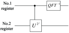
Figure 1: The sketch map for the procedure of phase estimation.

Recently, many researches on phase estimation have been presented including the lower bound for phase estimation 6 , optimal phase estimation for qubits in mixed states 7 , optimal phase measurements with pure Gaussian states 8 and optimal quantum circuits for general phase estimation 9 . However, the implementation of quantum phase estimation in physical systems is not a easy task since an unknown phase is involved in the procedure. To overcome this difficulty, we can introduce a fungible magnitude $T$ into the procedure of phase estimation. Solid-state system would be the best promising candidate for quantum computer considered by scientists. Recently one of the solid-state systems— quantum dot system attracts much attention because of its intrinsic properties. In the realm of quantum dot, electronic charge states 10a ; 10b , single-electron spin states 11a ; 11b , the spin singlet state and triple states of double electrons 12a ; 12b can all be used as qubit to encode quantum information. Especially, schemes combining cavity technology become very useful for quantum information processing because the cavity mode can be used as date-bus for long-distance information transfer or long-distance fast coupling between two arbitrary qubits. In comparison with other transmission medium, the parallel operations on two arbitrary different qubits can be more easily realized by using cavity technology. Moreover the spatial separation of electronic charge state can enhance quantum coherent 13 . Therefore we investigate the implementation of quantum phase estimation via the interaction between weakly coupled double quantum-dot molecules and microcavity in this paper. Because we introduce the new fungible magnitude, we can calculate time $T$ in terms of the final measurement result, which corresponds to the phase $\widetilde{\phi}$. Then we can calculate the error of time comparing with an ideal clock, if the error is within the range of the precision $\eta$ ($\eta=\widetilde{\phi}/\phi\times 100\%$) of phase estimation, the error will be neglected, otherwise, the frequency of time should be regulated.

II implementation of phase estimation and calibration of timepiece

In this section, we discuss a scenario for implementing quantum phase estimation in detail. During this process, we also can check a timepiece whether it is precise or not by comparing with an ideal timepiece.

II.1 Interaction between weakly coupled double quantum-dot molecule with laser fields and microcavity

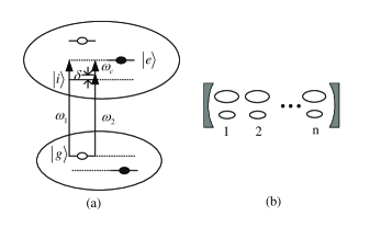
Figure 2: (a) Configuration of a weakly coupled double quantum-dot molecule. Two ellipses present two arbitrary quantum dots, the ground state denoted by $|g\rangle$ is used for the qubit logic state $|\widetilde{0}\rangle$, the excited state $|e\rangle$ for logic state $|\widetilde{1}\rangle$, and $|i\rangle$ is an intermediate state. $\omega_{1}$ and $\omega_{2}$ are two frequencies of pulse lasers, and $\omega_{c}$ is the frequency of cavity photon. (b) $n$ quantum-dot molecules are embedded in a microcavity. Assume that the distance between two neighboring quantum-dot molecules is large enough to neglect Coulomb correlations.

In our scheme, we use electronic charge (electron-hole pair) states to store information, the configuration diagram of a qubit is shown in Fig. 2 (a). The state $|g\rangle$, $|e\rangle$ and $|i\rangle$ are resulted from the conduction and valence band states of the two individual quantum dots with different sizes 10a . All of the quantum-dot molecules are embedded in a microcavity. Assume that there is no intermediate state between the two lowest conduction and the highest valance band state. If we perform a pulse laser on a coupled double quantum-dot molecule with frequency $\omega_{1}$, the Rabi transition $|g\rangle\leftrightarrow|e\rangle$ can be governed by the following interaction Hamiltonian ($\hbar=1$) 10a

$$H_{I}=\Omega_{1}(|e\rangle\langle g|e^{i\phi_{1}}+|g\rangle\langle e|e^{-i\phi_{1}}),$$ (1)

where $\Omega_{1}$ is the Rabi frequency, and $\phi_{1}$ is the laser phase. We can obtain the evolution after a duration time $t$

$$|g\rangle\rightarrow-ie^{-i\phi_{1}}\sin(\Omega_{1}t)|g\rangle+\cos(\Omega_{1}t)|e\rangle,$$ (2a)

$$|e\rangle\rightarrow\cos(\Omega_{1}t)|g\rangle-ie^{i\phi_{1}}\sin(\Omega_{1}t)|e\rangle,$$ (2b)

from which we can realize arbitrary single-qubit transformations by adjusting $\Omega_{1}$, $t$ and $\phi_{1}$.

If we switch on a pulse laser with frequency $\omega_{2}=E_{e}-E_{g}-\omega_{c}$, then the $\omega_{2}$ laser photon and the $\omega_{c}$ cavity photon will participate a resonant transition $|g\rangle\leftrightarrow|e\rangle$, the interaction Hamiltonian can be written as 10a

$$H_{II}=\Omega_{eff}(|e\rangle\langle g|ae^{i\phi_{2}}+|g\rangle\langle e|a^{{\dagger}}e^{-i\phi_{2}}),$$ (3)

where $\Omega_{eff}=\Omega_{c}\Omega_{2}/\delta$; $\delta=\omega_{2}-(E_{i}-E_{g})$ is the detuning between laser frequency and transition energy from $|g\rangle$ to $|e\rangle$ during this transition; $\Omega_{2}$ and $\Omega_{c}$ are the coupling strengths between $|g\rangle\leftrightarrow|i\rangle$ and $|i\rangle\leftrightarrow|e\rangle$, respectively. There is no occupation on the intermediate state $|i\rangle$ because of the existing large detuning $\delta$. We can obtain the time evolution corresponding to $H_{II}$ as

$$|g\rangle|0\rangle\rightarrow|g\rangle|0\rangle,$$ (4a)

$$|g\rangle|1\rangle\rightarrow\cos(\Omega_{eff}t)|g\rangle|1\rangle-ie^{i\phi_{2}}\sin(\Omega_{eff}t)|e\rangle|0\rangle,$$ (4b)

$$|e\rangle|0\rangle\rightarrow\cos(\Omega_{eff}t)|e\rangle|0\rangle-ie^{-i\phi_{2}}\sin(\Omega_{eff}t)|g\rangle|1\rangle,$$ (4c)

$$|e\rangle|1\rangle\rightarrow|e\rangle|1\rangle.$$ (4d)

This process of evolution is the essential ingredient to realized arbitrary two-qubit operations in this system, such as Controlled-not gate 10a and Controlled-phase-flip, where the photonic state ($|0\rangle$ or $|1\rangle$) is used to mediate the coupling between arbitrary two qubits.

II.2 Implementation of general quantum phase estimation

To implement quantum phase estimation, we prepare two clocks (clock 1 is a precise one, the frequency of clock 2 is unknown but it’s scale is well-proportioned), a vacuum microcavity mode state $|0\rangle$, and $m+1$ coupled double quantum-dot molecules without excess electron in their conduction bands, where $m$ molecules are all initialized in $|g\rangle^{\otimes m}=|\widetilde{0}\rangle^{\otimes m}$, and the $(m+1)$th molecule is in $|e\rangle_{m+1}=|\widetilde{1}\rangle_{m+1}$. The detailed scenario for implementing general quantum phase estimation can be described as the following in three steps:

(I) Firstly, perform a Hadamard gate operation on each of the quantum-dot molecules from molecule 1 to molecule $m$, respectively, which can be realized by the interaction as that in Eq. (1). Here we choose $\phi_{1}=2k\pi+\pi/2$ and $\Omega_{1}t/\hbar=2n\pi+\pi/4$, ($k,n\in\mathbb{N}$). The time $t$ is detected by clock 1. Then we should perform a controlled phase $C-U$ gate on quantum-dot molecules $m$ and $m+1$ (molecule $m$ is used as control bit while molecule $m+1$ as target bit) by the interaction as that in Eq. (3). However, molecule $m+1$ is remain in the state $|\widetilde{1}\rangle$ at all time, so we only need to operate a single-qubit $\phi$ phase gate on molecule $m$ to achieve above task ($C-U$ gate) by using the interaction as that in Eq. (1) by choosing $\Omega_{1}t/\hbar=2n\pi+\pi/2$ and $\phi_{1}=\phi+\pi/2$ (the $\phi$ is unknown and can be controlled by an unknown length $l$ of an electro-optic crystal, so it also can be controlled by the time $T$ of going through the electro-optic crystal). The time $T$ is detected by clock 2. Similarly, we perform 2 times $\phi$ phase transformations on molecule $m-1$, perform 4 times $\phi$ phase transformations on molecule $m-2$, $\cdots$, and perform $2^{m-1}$ times $\phi$ phase transformations on molecule 1. After that, the state of total system becomes

$$|\psi\rangle = \frac{1}{2^{m/2}}(|\widetilde{0}\rangle_{1}+e^{i2^{m-1}\phi}|\widetilde{1}\rangle_{1})(|\widetilde{0}\rangle_{2}+e^{i2^{m-2}\phi}|\widetilde{1}\rangle_{2})$$ (5)

$$\cdots(|\widetilde{0}\rangle_{m}+e^{i2^{0}\phi}|\widetilde{1}\rangle_{m})|\widetilde{1}\rangle_{m+1}$$

$$= \frac{1}{2^{m/2}}\sum_{k=0}^{2^{m}-1}e^{i\phi k}|k\rangle.$$

(II) Setting $\phi=2\pi\varphi$, assume that $\varphi$ can be expressed exactly in $m$ qubits, so $\varphi=0.\varphi_{1}\cdots\varphi_{m}$ ($\varphi_{i}=0$ or $1$), where $0.\varphi_{1}\cdots\varphi_{m}=\varphi_{1}/2+\varphi_{2}/4+\cdots+\varphi_{m}/2^{m}$. The state of quantum-dot molecules from molecule $1$ to molecule $m$ can be rewritten as

$$|\psi\rangle = \frac{1}{2^{m/2}}(|\widetilde{0}\rangle_{1}+e^{2\pi i0.\varphi_{m}}|\widetilde{1}\rangle_{1})(|\widetilde{0}\rangle_{2}+e^{2\pi i0.\varphi_{m-1}\varphi_{m}}|\widetilde{1}\rangle_{2})$$ (6)

$$\cdots(|\widetilde{0}\rangle_{m}+e^{2\pi i0.\varphi_{1}\cdots\varphi_{m}}|\widetilde{1}\rangle_{m}).$$

Then perform a inversed QFT on the No.1 register, the detailed process can be described as following. (1) we perform a Hadamard transform on quantum-dot molecule 1, the state of quantum-dot molecule 1 becomes $|\varphi_{m}\rangle$. (2) we perform a series of operations on quantum-dot molecules 1 and 2: we perform a single-qubit $-\theta$ ($\theta=\pi/4$) phase gate operation on quantum-dot molecule 1, a Controlled-not gate operation on quantum-dot molecules 1 and 2 (molecule 1 is used as control bit while molecule 2 as target bit), a single-qubit $\theta$ phase gate operation on molecule 2, a Controlled-not gate operation on quantum-dot molecules 1 and 2 again, and a single-qubit $-\theta$ phase gate operation on molecule 2. These operations on molecules 1 and 2 can be expressed by a total transformation $U_{12}=U_{2}(-\theta)U_{12}(cnot)U_{2}(\theta)U_{12}(cnot)U_{1}(-\theta)$. Then we perform a Hadamard transform on quantum-dot molecule 2. The state of quantum-dot molecule 2 becomes $|\varphi_{m-1}\rangle$. (3) Similarly, we apply the transformation $U_{13}$ on molecules 1 and 3 with $\theta=\pi/8$, and the transformation $U_{23}$ on molecules 2 and 3 with $\theta=\pi/4$ as the step (2). Then we perform a Hadamard transform on quantum-dot molecule 3. The state of quantum-dot molecule 2 becomes $|\varphi_{m-2}\rangle$; $\cdots$; (m) We apply the transformation $U_{1m}$ on molecules 1 and $m$ with $\theta=\pi/2^{m-2}$, the transformation $U_{2m}$ on molecules 2 and $m$ with $\theta=\pi/2^{m-3}$, $\cdots$, and the transformation $U_{m-1,m}$ on molecules $m-1$ and $m$ with $\theta=\pi/4$ as the step (2). Finally, we perform a Hadamard transformation on quantum-dot molecule $m$. The state of quantum-dot molecule $m$ becomes $|\varphi_{1}\rangle$.

(III) We detect the quantum-dot molecules 1, 2, $\cdots$, $m$ by detectors, and read out the result in reversed order. The measurement result is $|\varphi_{m}\varphi_{m-1}\cdots\varphi_{1}\rangle$, but readout is $|\varphi_{1}\varphi_{2}\cdots\varphi_{m}\rangle$, so the estimated phase $\widetilde{\phi}=\phi=2\pi 0.\varphi_{1}\cdots\varphi_{m}$, which is precise.

II.3 Remarks on phase estimation and calibration of timepiece

In above process, we have assumed that $\varphi$ can be expressed exactly in $\kappa=m$ qubits, but it is only an ideal case. For an arbitrary value of $\varphi$, and $\kappa<m$, if we wish to approximate $\varphi$ up to an accuracy of $1/2^{n}$, then the successful probability should be about $1-1/(2^{m-n+1}-4)$ with $m\geq n+1$. The unknown phase $\varphi$ can be created by modulating the length $l=vT$ of an electro-optic crystal (such as KDP crystal), so we can estimate the time $T$ in terms of $\phi_{1}=2\pi\varphi+\pi/2=\varpi n^{3}_{0}vr_{63}ET/2c=\varpi n^{2}_{0}nr_{63}ET/2$, where $\varpi$ is the frequency of electric field, $r_{63}$ is electro-optic tensor, $v$ is the velocity of laser through the electro-optic crystal, and $n$ and $n_{0}$ are refractive rates for vacuum and electro-optic crystal, respectively. In the process of implementing phase estimation, the time $T$ is detected by clock 2, if the clock 2 undergoes $h$ scales of total $O$ scales, we can calculate the total time by $T_{total}=OT/h$ around a circle in clock 2. In the ideal case, we compare the $T_{total}$ with the time $T_{i}$ around a circle for the idea clock. If $T_{total}=T_{i}$, clock 2 is an accurate one, otherwise, the frequency of clock 2 should be regulated. In the general case, we should first determinate the error of phase $\eta=\widetilde{\phi}/\phi\times 100\%$, then we can calculate the error $\eta^{\prime}=T_{total}/T_{i}\times 100\%$ of clock 2. If $\eta^{\prime}\leq\eta$, we can treat clock 2 as an accurate one, otherwise, the frequency of clock 2 has to be regulated. In the case of $T_{total}<T_{i}$, the frequency of clock 2 should be increased, otherwise, the frequency should be decreased. In a word, calibrate of timepiece includes two aspects: one is checking whether the clock 2 is precise or not, the other is if the clock 2 is not precise, we will regulate the frequency of clock 2 according to the error of estimated phase. Similarly, we also can estimate the length $l$ of electro-optic crystal based on the procedure of quantum phase estimation.

III discussions and conclusions

We then discuss the feasibility of the current scheme with experimental parameters reported in current experiments. For general weakly coupled double quantum-dot molecule, the coupling strength $t$ between $|e\rangle$ and $|i\rangle$ is about $0.01meV$, and the energy difference $\Delta=E_{e}-E_{i}$ is about $10meV$, thus the spatial separation factor $\gamma=t^{2}/(\Delta^{2}+t^{2})\simeq 10^{-6}$ 10a . In our scheme, we use two laser pluses with different coupling strength $\Omega_{1}$, $\Omega_{2}$, which will satisfy the condition $\Omega_{1}\sim 10^{-3}\Omega_{2}$ according to the above value of $\gamma$. For the process of the interaction involves two photons, the coupling strength $\Omega_{c}$ caused by cavity field is $300MHz$ 10b ; 11b , where we have assumed that $\Omega_{2}=0.1meV$ and $\delta=1meV$ as done in Ref. 10a , resulting in $\Omega_{eff}=\Omega_{2}\Omega_{c}/\delta\simeq 30KHz$ and $\Omega_{1}\simeq 10^{-4}meV$. Therefore completion of a single-qubit operation and a two-qubit operation will cost about several hundreds nanosecond and $10^{-4}s$, respectively. We can calculate the total time for completing the current scheme, which is about $T=n(n-1)/2\times 10^{-4}s$. The coherent time of the spatial separate charge qubits can reach tens of second 13 (we can assume $T_{c}=10s$). Comparing the time $T$ with $T_{c}$, it is shown that the number of qubit will be $n\simeq 450\gg 100$ if $T=T_{c}$, so our scheme is suitable for large-scale quantum computation in quantum dot system.

In conclusion, we present a scenario for implementing general quantum phase estimation via weakly coupled double quantum-dot molecules embedded in a microcavity. The involved two quantum dots are not necessarily to be exactly identical, which reduces the experimental difficulty. In the same process of our implementation of quantum phase estimation, we can also realize the calibration of timepiece or estimation of length. The key ingredient for our scheme is to implement the $C-U$ transformation and the reversed QFT. In addition, the error of time (length) can be calculated by the fidelity of quantum phase. In other words, arbitrary classical quantity related to the estimated quantum phase can be estimated by the same method. These classical estimation results (time $T$, length $l$, et al) are useful for our lives. The phase estimation would be also an important step for fabricating quantum computer since it is the key ingredient for complex quantum algorithms. It also deserves to note that our idea can be generalized to other systems, such as atom system, trapped ion system and linear optic system.

- (1) C. H. Bennett and G. Brassard, in Proceedings of the IEEE International Conference on Computers, System, and signal Processing, Bangalore, India, 1984.
- (2) V. Karimipour and A. T. Rezakhani, Phys. Rev. A 66, 052111 (2002).
- (3) R. G. Unanyan and M. Fleischhauer, Phys. Rev. A 69, 050302 (2004).
- (4) P. W. Shor, Algorithms for quantum computation: discrete logarithms and factoring, in Proceedings, 35th Annual Symposium on Foundations of Computer Science, IEEE Press, Los Alamitos, CA, 1994.
- (5) P. Jaksch and A. Papageorgiou, Phys. Rev. Lett. 91, 257902 (2003).
- (6) D. S. Abrams and S. Lloyod, Phys. Rev. Lett. 83, 5162 (1999).
- (7) M. A. Nielsen and I. L. Chuang, Quantum Computation and Quantum Information, Cambridge University Press, Cambridge, England, 2000.
- (8) A. J. Bessen, Phys. Rev. A 71, 042313 (2005).
- (9) G. M. D’riano, C. Macchiavello, and P. Perinotti, Phys. Rev. A 72, 042327 (2005).
- (10) A. Monras, Phys. Rev. A 73, 033821 (2006).
- (11) W. v. Dam, G. M. D’Ariano, A. Ekert, C. Macchiavello, and M. Mosca, Phys. Rev. Lett. 98, 090501 (2007).
- (12) X. Q. Li, and Y. Yan, Phys. Rev. B 65, 205301 (2002).
- (13) M. S. Sherwin, A. Imamoglu, and T. Montroy, Phys. Rev. A 60, 3508 (1999).
- (14) D. Loss, and D. P. DiVincenzo, Phys. Rev. A 57, 120 (1998).
- (15) A. Imamoglu, D. D. Awschalom, G. Burkard, D. P. DiVincenzo, D. Loss, M. Sherwin and A. Small, Phys. Rev. Lett. 83, 4204 (1999).
- (16) D. Stepanenko, and G. Burkard, Phys. Rev. B 75, 085324 (2007).
- (17) R. Hanson, and G. Burkard, Phys. Rev. Lett. 98, 050502 (2007).
- (18) X. Q. Li and Y. Arakawa, Phys. Rev. A 63, 012302 (2000).