The spin-1/2 Ising model on the bow-tie lattice
as an exactly soluble free-fermion model

Abstract

The spin-1/2 Ising model on the bow-tie lattice is exactly solved by establishing a precise mapping relationship with its corresponding free-fermion eight-vertex model. Ground-state and finite-temperature phase diagrams are obtained for the anisotropic bow-tie lattice with three different exchange interactions along three different spatial directions.

05.50.+q, 68.35.Rh

1 Introduction

The planar Ising models represent a prominent class of exactly soluble lattice-statistical models, which exhibit remarkable phase transitions [1]. Despite the universality of their critical behaviour, it is still of great research interest to analyze accurately the critical behaviour of a specific lattice with particular interactions. As a matter of fact, the competition between particular interactions might for instance lead to an existence of reentrant phase transitions, which have been precisely confirmed in the spin-1/2 Ising model on the anisotropic union jack (centered square) lattice [2]. In the present work, we shall provide the exact solution for the spin-1/2 Ising model on the anisotropic bow-tie lattice.

2 Model and its exact solution

Consider the spin-1/2 Ising model on the bow-tie lattice schematically shown in Fig. 1. The model under investigation is given by Hamiltonian

$${\cal H}=-J_{1}\sum_{(i,j)}\sigma_{i}\mu_{j}-J_{2}\sum_{(k,l)}\sigma_{k}\mu_{l}-J_{3}\sum_{(m,n)}\sigma_{m}\sigma_{n},$$ (1)

where the Ising spins $\sigma_{i}=\pm 1/2$ and $\mu_{j}=\pm 1/2$ are used to distinguish two kinds of inequivalent lattice sites depicted in Fig. 1 as full and empty circles, respectively,

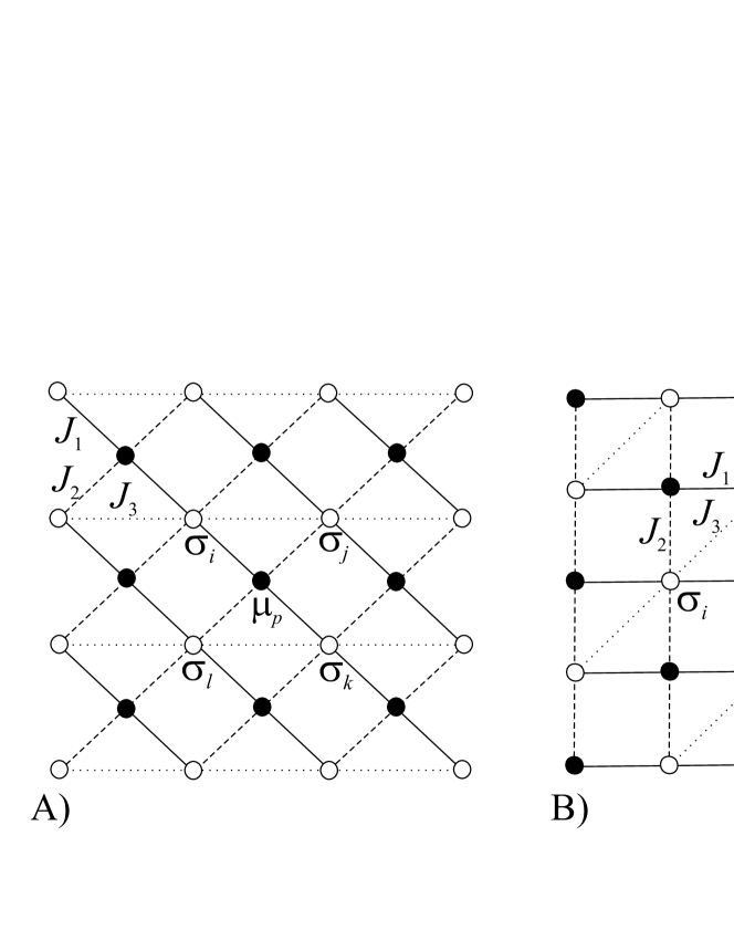
Figure 1: A) The magnetic structure of the spin-1/2 Ising model on the bow-tie lattice. The full and empty circles illustrate lattice positions of two inequivalent $\sigma_{i}$ and $\mu_{j}$ spin sites, respectively. Solid, dashed and dotted lines schematically represent pairwise spin-spin interactions $J_{1}$, $J_{2}$ and $J_{3}$ along three different spatial directions. B) The bow-tie lattice and its relation with the square lattice.

while the parameters $J_{i}$ ($i=1-3$) denote pairwise spin-spin interactions along three different spatial directions. For further convenience, the total Hamiltonian (1) can be rewritten as a sum of plaquette Hamiltonians, ${\cal H}=\sum_{p=1}^{N}{\cal H}_{p}$, where each plaquette Hamiltonian

$${\cal H}_{p}=-J_{1}\mu_{p}(\sigma_{i}+\sigma_{k})-J_{2}\mu_{p}(\sigma_{j}+\sigma_{l})-J_{3}\left(\sigma_{i}\sigma_{j}+\sigma_{k}\sigma_{l}\right)/2,$$ (2)

involves all interactions terms of one square plaquette with the Ising spin $\mu_{p}$ in its centre (the factor 1/2 in the last expression avoids a double counting of the interaction $J_{3}$). In the consequence of that, the partition function of the spin-1/2 Ising model on the bow-tie lattice can be partially factorized

$${\cal Z}=\sum_{\{\sigma_{i}\}}\prod_{p=1}^{N}\sum_{\mu_{p}=\pm 1/2}\!\!\!\!\!\exp(-\beta{\cal H}_{p})=\sum_{\{\sigma_{i}\}}\prod_{p=1}^{N}\omega_{p}(\sigma_{i},\sigma_{j},\sigma_{k},\sigma_{l}).$$ (3)

Above, $\beta=1/(k_{\rm B}T)$, $k_{\rm B}$ labels the Boltzmann’s constant, $T$ is absolute temperature and the Boltzmann’s factor $\omega(\sigma_{i},\sigma_{j},\sigma_{k},\sigma_{l})$ is given by

$$\omega(a,b,c,d)=2\exp\left[\frac{\beta J_{3}}{2}\left(ab+cd\right)\right]\cosh\left[\frac{\beta J_{1}}{2}\left(a+c\right)+\frac{\beta J_{2}}{2}\left(b+d\right)\right].$$ (4)

Due to the spin reversal symmetry, there are at best eight different Boltzmann’s weights to be obtained from Eq. (4) by substituting sixteen allowed spin configurations of four corner spins of each square plaquette

$$\omega_{1}(+,+,+,+)\!\! = \!\!2\exp\left(\frac{\beta J_{3}}{4}\right)\cosh\left[\frac{\beta}{2}\left(J_{1}+J_{2}\right)\right],$$

$$\omega_{2}(+,-,+,-)\!\! = \!\!2\exp\left(-\frac{\beta J_{3}}{4}\right)\cosh\left[\frac{\beta}{2}\left(J_{1}-J_{2}\right)\right],$$

$$\omega_{3}(+,-,-,+)\!\! = \!\!2\exp\left(-\frac{\beta J_{3}}{4}\right),\quad\omega_{4}(+,+,-,-)=2\exp\left(\frac{\beta J_{3}}{4}\right),$$

$$\omega_{5}(+,-,+,+)\!\! = \!\!\omega_{6}(+,+,+,-)=2\cosh\left(\frac{\beta J_{1}}{2}\right),$$

$$\omega_{7}(+,+,-,+)\!\! = \!\!\omega_{8}(-,+,+,+)=2\cosh\left(\frac{\beta J_{2}}{2}\right).$$ (5)

In this respect, the Boltzmann’s weights (5) can readily be regarded as the effective Boltzmann’s weights of the corresponding eight-vertex model on a square lattice. It can be easily proved, moreover, that the Boltzmann’s weights (5) satisfy the free-fermion condition ($\omega_{1}\omega_{2}+\omega_{3}\omega_{4}=\omega_{5}\omega_{6}+\omega_{7}\omega_{8}$) and thus, the spin-1/2 Ising model on the bow-tie lattice is effectively mapped to the free-fermion eight-vertex model solved by Fan and Wu [3]. The critical condition of the free-fermion eight-vertex model $\omega_{1}+\omega_{2}+\omega_{3}+\omega_{4}=2{\rm max}\{\omega_{1},\omega_{2},\omega_{3},\omega_{4}\}$ then determines the criticality of the spin-1/2 Ising model on the bow-tie lattice provided that the Boltzmann’s weights are chosen according to Eq. (5). In our case, the largest Boltzmann’s weight is either $\omega_{1}$ or $\omega_{2}$. Accordingly, if $\omega_{1}>\omega_{2}$ then the critical condition reads

$$\exp\left(\frac{\beta_{\rm C}J_{3}}{2}\right)=\frac{\cosh\left[\frac{\beta_{\rm C}}{2}\left(J_{1}-J_{2}\right)\right]+1}{\cosh\left[\frac{\beta_{\rm C}}{2}\left(J_{1}+J_{2}\right)\right]-1},$$ (6)

otherwise

$$\exp\left(\frac{\beta_{\rm C}J_{3}}{2}\right)=\frac{\cosh\left[\frac{\beta_{\rm C}}{2}\left(J_{1}-J_{2}\right)\right]-1}{\cosh\left[\frac{\beta_{\rm C}}{2}\left(J_{1}+J_{2}\right)\right]+1},$$ (7)

where $\beta_{\rm C}=1/(k_{\rm B}T_{\rm C})$ and $T_{\rm C}$ is the critical temperature.

3 Results and discussions

The most interesting numerical results for the spin-1/2 Ising model on the bow-tie lattice are displayed in Fig. 2. Fig. 2A) illustrates the ground-state phase diagram

Figure 2: A) Ground-state phase diagram in the $J_{2}-J_{3}$ plane for $J_{1}>0$. Squares show a typical spin configuration of the basic unit cell of bow-tie lattice within each sector of the phase diagram. The phase diagram for $J_{1}<0$ case can be obtained by making mirror image of Fig. 2A) with respect to $J_{2}=0$ axis. B) Critical temperature as a function of $J_{3}/|J_{1}|$ for several values of the ratio $J_{2}/|J_{1}|$.

with all possible spin configurations that might appear in the model under investigation. Furthermore, Fig. 2B) shows variations of the critical temperature with the ratio $J_{3}/|J_{1}|$ at several fixed values of $J_{2}/|J_{1}|$. It is quite obvious from this figure that the finite-temperature phase diagram consists of two wings of critical lines (each corresponds to one ordered phase), which merge together with infinite gradient at the $T_{\rm C}=0$ axis whenever $|J_{2}|\neq|J_{1}|$. Owing to this fact, the spin-1/2 Ising model on the anisotropic bow-tie lattice cannot exhibit similar reentrant phase transitions as does the analogous spin-1/2 Ising model on the union jack lattice with a high probability because of its over-frustration [2]. It is noteworthy that single critical lines, which are shown in Fig. 2B) as broken lines, represent the critical lines for two special cases with $|J_{2}|=|J_{1}|$. Under this condition, the competing interactions give rise to the disordered phase, which appears in the whole parameter space $|J_{3}|>2|J_{1}|$ due to a strong geometric frustration inherent in the topology of bow-tie lattice.

References

• [1] R. J. Baxter, Exactly solved models in statistical mechanics, 3rd ed., Academic Press, London, 1989.
• [2] T. Chikyu and M. Suzuki, Progr. Theor. Phys. 22, 1242 (1987) and references cited therein.
• [3] C. Fan and F. Y. Wu, Phys. Rev. B 2, 723 (1970).