Biexciton stability in carbon nanotubes

Abstract

We have applied the quantum Monte Carlo method and tight-binding modelling to calculate the binding energy of biexcitons in semiconductor carbon nanotubes for a wide range of diameters and chiralities. For typical nanotube diameters we find that biexciton binding energies are much larger than previously predicted from variational methods, which easily brings the biexciton binding energy above the room temperature threshold.

Size-dependent optical excitations in nano-structures are at the heart of fundamental studies as well as conceivable applications scholes:06 . Carbon nanotubes (CNTs) make no exception, showing very sensitive electronic and optical properties to the atomic structure and spanning a wide range of wavelengths bachilo:02 . The stability of the excitonic states, neutral or charged optically excited electron-hole complexes, is determined by their binding energy with respect to thermal fluctuations. In quasi-1D systems, the binding energy can be much larger than in systems of higher dimensionality. In inorganic semiconductor heterostructures, for instance, the exciton binding energy $E_{b}^{\mbox{\tiny X}}$ is substantially larger than someya:96 ; ogawa:91 ; rossi:97 the binding energy $4\,Ry^{*}$ in a strictly 2D system bastard:82 , where $Ry^{*}$ is the Rydberg energy of the host material. Analogously, the biexciton binding energy $E_{b}^{\mbox{\tiny XX}}$ of two electron-hole pairs, optically excited in a two-photon process, is not limited banyai:87 ; baars:98 to its 2D value of $0.77\,Ry^{*}$ usukura:99 ; hohenester:05 .

Since CNTs are quasi-1D systems, obtained by rolling up a graphene sheet saito:98 , they are characterized by rather large binding energies wang:05 ; maultzsch:05 , analogously to conjugated polymers rohlfing:99 ; ruini:02 . On the other hand, in CNTs one expects strongly diameter-dependent binding energies. Indeed, in addition to the increase of the ratio $E_{b}^{\mbox{\tiny X(XX)}}/Ry^{*}$ with decreasing diameter, due to the transition from a quasi-2D system to a quasi-1D system, also electron and hole effective masses, which determine $Ry^{*}$, change with the CNT diameter. Furthermore, due to the involved energy scales, in CNTs not only excitons but also biexcitons might be stable against thermal fluctuations at room temperature; also, the energy separation can be larger then the linewidth, and optical detection of biexcitons should be possible. Contrary to inorganic semiconductors and semiconductor nanostructures, where biexcitons have received considerable interest, there is only very little work devoted to biexcitons in CNTs. Following the pioneering work of Ando ando:97 , the exciton binding energy has been calculated for several nanotubes, with different diameter and chirality, both within ab initio approaches chang:04 ; spataru:04 and semiempirical methods perebeinos:04 ; zhao:04 ; pedersen:03 ; kane:03 ; capaz:06 ; jiang:07 . On the contrary, the biexciton binding energy, which is presently not accessible to the more accurate first principles methods, has been computed only via an approximate variational approach pedersen:05 .

In this paper we use the quantum Monte Carlo (QMC) method to calculate the exact (dimensionless) binding energy $E_{b}^{\mbox{\tiny XX}}/Ry^{*}$ of biexcitons confined to the surface of a cylinder of diameter $D$. We find that the biexciton is much more stable and its binding energy much larger than estimated from variational methods, particularly for intermediate to large $D/a_{B}^{*}$. Assuming homogeneous dielectric screening and tight-binding estimates for the CNT effective masses, we also estimate $E_{b}^{\mbox{\tiny XX}}$ for several families of CNTs. We find that for realistic values of the dielectric constant, $E_{b}^{\mbox{\tiny XX}}$ can be comparable or larger than $k_{B}T_{\mbox{\tiny room}}$ even for the larger CNT diameters.

Let us consider electrons and holes confined to the surface of an infinitely long cylinder of diameter $D$, as indicated in Fig. 1. It is convenient to use dimensionless exciton units, where $\hbar=1$, and in which masses are measured in units of the reduced electron-hole mass $\mu$, distances in units of the effective Bohr radius $a_{B}^{*}=(\epsilon/\mu)a_{B}$, and energies in units of the effective Rydberg $Ry^{*}=e^{2}/(2\epsilon a_{B}^{*})$. With the approximation of equal electron and hole effective masses pedersen:03 ; perebeinos:04 ; comment.mass , the biexciton Hamiltonian in dimensionless units reads

$$H = -\frac{1}{2}(\nabla_{1}^{2}+\nabla_{2}^{2}+\nabla_{a}^{2}+\nabla_{b}^{2})$$ (1)

$$-\frac{2}{r_{1a}}-\frac{2}{r_{1b}}-\frac{2}{r_{2a}}-\frac{2}{r_{2b}}+\frac{2}{r_{12}}+\frac{2}{r_{ab}}\,,$$

Here, $\bm{r}_{1}$,$\bm{r}_{2}$ ($\bm{r}_{a}$,$\bm{r}_{b}$) are the positions of the two electrons (holes),and $r_{ij}$ is the distance between particles $i$ and $j$. We choose electrons (holes) with opposite spin orientations and consider the optically active spin-singlet biexciton ground state.

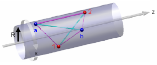
Figure 1: Biexciton complex on a cylindrical surface. $x$ is the circumferential and $z$ the longitudinal direction of the tube with diameter $D=2R$. Particles $1,2$ (electrons) and $a,b$ (holes) are confined to the surface and form a spin singlet state.

Variational QMC.—In the following we sketch our numerical approach. In addition to exact QMC calculations, to be discussed below, we have performed variational QMC (VQMC) calculations. We have exploited the (unnormalized) Hylleraas–Ore trial wavefunction hylleraas:46 in a slightly modified version

$$\Psi_{T}=e^{-\frac{1}{2}(s_{1a}+s_{1b}+s_{2a}+s_{2b})}\cosh[\frac{\beta}{2}(s_{1a}-s_{1b}+s_{2b}-s_{2a})]\,.$$ (2)

Here, the $s_{ij}$’s are relative distances scaled by variational parameters. As we employ cylindrical coordinates, the expression for $s_{ij}$ reads

$$s_{ij}=\sqrt{\left(\frac{D\sin{(x_{ij}/D)}}{q}\right)^{2}+\left(\frac{z_{ij}}{k}\right)^{2}}\,,$$ (3)

where $x$ and $z$ are oriented along the circumference and the symmetry axis of the cylinder, respectively (see Fig. 1). Variational parameters $q$ and $k$ allow for different scaling for both directions pedersen:03 . $\beta$ is an additional variational parameter determining the strength of the coupling between the two excitonic complexes of a biexciton, where $\beta=1$ corresponds to two separate excitons, and for $\beta=0$ there is equal binding within all electron-hole pairs. The variational parameters $q$, $k$ and $\beta$ have to be determined such that the total energy $E_{T}=\langle\Psi|H|\Psi\rangle/\langle\Psi|\Psi\rangle$ becomes minimized.

Quite generally, after separation of the biexciton center-of-mass motion, the calculation of $E_{T}$ involves six-fold integrals, which constitutes a formidable computational task. The calculation of $E_{T}$ is performed by the VQMC approach thijssen:99 , whose main elements can be summarized as follows: since the trial wavefunction (2) of the optically active spin-singlet biexciton groundstate is always positive (thereby avoiding the fermionic sign problem), it can be represented by an ensemble of “walkers”, each one characterized by the particle positions $\bm{r}_{1}$, $\bm{r}_{2}$, $\bm{r}_{a}$, $\bm{r}_{b}$. Starting from a suitable initial configuration, one generates a Markov chain for the walkers where the probability for a specific configuration is given by $\Psi_{T}^{2}(\bm{r}_{1},\bm{r}_{2},\bm{r}_{a},\bm{r}_{b})$. Upon sampling of the “local energy” $E_{L}=H\Psi_{T}/\Psi_{T}$ one then obtains the energy $E_{T}$ associated to the trial wavefunction thijssen:99 . Let us denote the ensemble of walkers with $\rho(\bm{r}_{1},\bm{r}_{2},\bm{r}_{a},\bm{r}_{b},t)$, where $t$ is a fictitious time. The Fokker-Planck equation, which in our dimensionless units reads

$$\frac{\partial\rho}{\partial t}=\frac{1}{4}\sum_{i=1,2,a,b}{\nabla_{i}\left(\nabla_{i}-\bm{F}_{i}\right)}{}\rho,$$ (4)

in time-discretized form defines a scheme to proceed from a configuration $\rho(t)$ to $\rho(t+\delta t)$ according to the drift and diffusion process given on the right-hand side comment.drift . Thus, the VQMC simulation consists of the three main steps of (i) initialization of the ensemble of walkers, (ii) drift and diffusion of all particles in each walker according to Eq. (4), and (iii) sampling of the local energy $E_{L}$ once the stationary distribution is reached.

Guide Function QMC.—A slight variant of the VQMC approach allows for the exact solution of the Schrödinger equation. Let $\rho=\Psi\overline{\Psi}_{T}$ denote a function composed of the exact wavefunction $\Psi$ and the guide function $\overline{\Psi}_{T}$. The Fokker-Planck-type equation

$$\frac{\partial\rho}{\partial t}=\frac{1}{4}\sum_{i=1,2,a,b}{\nabla_{i}\left(\nabla_{i}-\bm{F}_{i}\right)}{}\rho-\left[E_{L}-E\right]\rho$$ (5)

in time-discretized form again defines a scheme that can be solved by means of Monte-Carlo sampling. It can be easily proven thijssen:99 that under stationary conditions Eq. (5) reduces to the exact Schrödiger equation. Thus, once the invariant $\rho$ is obtained the exact wavefunction is at hand. We represent $\rho$ by an ensemble of walkers, and account on the right-hand side of Eq. (5) for the first term through drift and diffusion and for the second term through a Monte-Carlo branching with probability $p=\exp[-(E_{L}-E)\delta t]$. Depending on the value of $p$, the walker dies, survives, or gives birth to other walkers thijssen:99 . In the simulation the energy $E$ is chosen such that the total number of walkers remains approximately constant and a constant distribution $\rho$ is reached. This invariant distribution and $E$ then determine the biexciton wavefunction and energy, respectively. Therefore, the main steps of this so-called guide function QMC approach are (i) initialization of the ensemble of walkers, (ii) drift and diffusion of all particles in each walker, (iii) branching of the walkers, and (iv) sampling of the wavefunction once the stationary distribution is reached.

Technically, one needs to choose $\delta t$ sufficiently small to allow for the separate drift-diffusion and branching steps accounting for the two different terms on the right-hand side of Eq. (5) tech-note ; $\overline{\Psi}_{T}$ has to be chosen such that the local energy $E_{L}$ in Eq. (5) remains finite when two particles in a walker approach each other. While this is guaranteed for the true wavefunction, $\overline{\Psi}_{T}$ is usually taken as a Jastrow-type wavefunction with the correct cusp condition jastrow:55 ; thijssen:99 . In practice we use $\overline{\Psi}_{T}=\Psi_{T}$ with $q=k=\frac{1}{4}$, $\beta=0$. We finally emphasize that both the VQMC and the exact QMC simulations can be applied in a straightforward manner to excitons, in which case the trial wavefunction is of the form $\Psi_{T}(\bm{r}_{1},\bm{r}_{a})=\exp[-s_{1a}]$ and $\overline{\Psi}_{T}=\exp[-2r_{1a}]$, respectively.

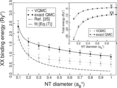
Figure 2: Biexciton binding energies as a function of CNT diameter, calculated with exact guide function QMC (black dots) and VQMC method (grey triangles). Statistical error bars of both methods are shown. The solid, black line is the result of using our fitting functions in Eq. (7). Inset: total energy of exciton and biexciton. Note that here $E^{\mbox{\tiny X}}=-E_{b}^{\mbox{\tiny X}}$.

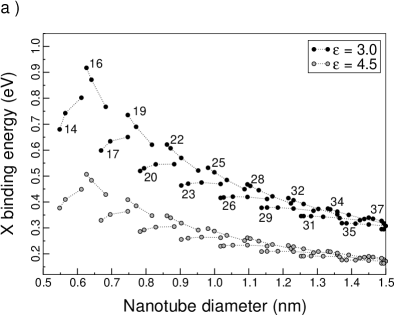
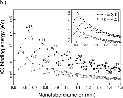
Figure 3: Exciton (a) and biexciton (b) binding energies as a function of CNT diameter and chirality. Inset: biexciton energies ($-E^{\mbox{\tiny XX}}$) in absolute units. The labels indicate the (2n+m) families, where (n,m) are the chiral indices of the NT.

Results.—In the inset of Fig. 2 we show the dimensionless total energies $E^{\mbox{\tiny X}}$ and $E^{\mbox{\tiny XX}}$ with respect to the band gap ($E_{g}=0$), calculated exactly by the guide function QMC method. As can be seen, the exciton energy $E^{\mbox{\tiny X}}$ shows the correct behaviour at infinite diameter, that is the 2D limit, where it converges to $-4\,Ry^{*}$ bastard:82 , while it is strongly red-shifted as the diameter is decreased due to the larger binding of the electron-hole pair, showing the transition from a quasi-2D to a quasi-1D system. Analogously, the biexciton energy $E^{\mbox{\tiny XX}}$ red-shifts as a result of the increased interaction of the two electron-hole pairs.

In order to investigate the stability of the biexciton complex with respect to the formation of separated excitons, we show in Fig. 2 the exact biexciton binding energy $E_{b}^{\mbox{\tiny XX}}$ for arbitrary dimensionless diameter $D/a^{*}_{B}$, along with the VQMC results and the fitting function of Ref. pedersen:05, . The biexciton results to be stable ($E_{b}^{\mbox{\tiny XX}}>0$) at any diameter, and it shows the expected limiting behaviour at infinite diameter, that is the 2D limit $0.77\,Ry^{*}$ usukura:99 . The binding energy increases with decreasing diameter, showing again the transition from a quasi-2D to a quasi-1D system. As can be noted, both variational results severely underestimate the binding energy in the whole range of diameters except for very small values. Moreover, they do not show the correct 2D limiting behavior. Such shortcoming of Hylleraas-Ore-type wavefunctions is in agreement with corresponding calculations for two-dimensional quantum wells heller:97 ; usukura:99 . To give a rough estimate, for typical CNT diameters of $D=0.8\div 1.2$ nm and using the dielectric constant $\epsilon=3.5$ given in Ref. pedersen:05, the excitonic units are $a^{*}_{B}=2.5\div 5.5$ nm and $Ry^{*}=0.04\div 0.08$ eV. This brings $E_{b}^{\mbox{\tiny XX}}$ into the $0.06\div 0.12$ eV range, which is $1.5\div 2.5$ larger than the variational results reported in Fig. 2.

In order to calculate exciton (X) and biexciton (XX) absolute energies explicitly, we assume that excitonic effects (X or XX binding) can be decoupled from band structure effects. We can therefore write the energies as

$$E^{\chi}=f^{\chi}(D/a_{B}^{*})Ry^{*}(D)\,,$$ (6)

where $\chi\in\{\mbox{\scriptsize X},\mbox{\scriptsize XX}\}$ and $f^{\chi}(x)$ is the exact dimensionless excitonic or biexcitonic energy shown in the inset of Fig. 2. We provide below a fitting function for $f^{\chi}(x)$, which allows us to calculate absolute binding energies for an arbitrary diameter,

$$f^{\chi}(x)=\left(a_{\chi}x^{-1}+b_{\chi}x^{-2}+c_{\chi}x^{-3}\right)\exp(-d_{\chi}x)+f^{\chi}_{\mbox{\tiny 2D}}\,,$$ (7)

where $f^{\chi}_{\mbox{\tiny 2D}}$ is the correct 2D limit, and $a_{\chi},b_{\chi},c_{\chi},d_{\chi}$ are the fitting parameters summarized in table I. The quality of the fit is proven by calculating the biexciton binding energy with $2f^{\mbox{\tiny X}}-f^{\mbox{\tiny XX}}$, see solid black line in Fig. 2.

We calculate the Rydberg energy $Ry^{*}$ from the tight-binding model of Ref. jorio:05, , which provides explicit fitting functions [Eq. (2) of Ref. jorio:05, ] for the electron and hole effective masses of semiconducting CNTs of arbitrary chirality and diameter. For the dielectric screenig entering $Ry^{*}$, we adopt the simplest screening model, in which all Coulomb interactions are reduced to an effective static dielectric constant $\epsilon$, following current literature pedersen:03 ; perebeinos:04 ; zhao:04 ; maultzsch:05 . This approximation, which proved to be successful in comparison with both experiments wang:06 and ab-initio calculations capaz:06 , is particularly suitable for embedding media with large dielectric constant, i.e. $\epsilon\gtrsim 3$, where the dielectric response is dominated by that of the medium rather then by the CNT polarizability jiang:07 .

Figure 3 shows Kataura-like plots for both exciton (a) and biexciton (b) binding energies in absolute units, in the $0.5\div 1.5$-nm diameter range, calculated from Eq. (6) and for different value of $\epsilon$. As expected, both X and XX energies decrease with increasing tube diameter, as follows from the behaviour of $f^{\chi}(x)$. The chirality effects, entering through the effective masses, introduce a modulation in the binding energy dependence on the diameter, significantly spreading out the binding energies for the range of diameters considered. As shown in Fig. 3(b), however, the biexciton binding energy is predicted to be above the $k_{B}T_{\mbox{\tiny room}}$ threshold (26 meV) even for the largest CNTs.

In summary, we have performed QMC calculations of the singlet optically active biexciton binding energy for CNTs of arbitrary diameter and chirality. The biexciton has been found to be always stable at room temperature in typical dielectric environments. We have also developed a scheme which allows us to calculate the exact exciton and biexciton binding energies through a simple fitting function approach, which includes the strong correlation effects exactly and the band-structure effects within a tight-binding approach.

Table 1: Fitting parameters in Eq. (7) for exciton (X) and biexciton (XX) energies in dimensionless exciton units.

	$a_{\chi}$	$b_{\chi}$	$c_{\chi}$	$d_{\chi}$	$f^{\chi}_{\mbox{\tiny 2D}}$
X	-2.62	0.3024	-0.01504	2.795	-4.00
XX	-5.08	0.56	-0.02832	2.345	-8.77

References

- (1) G. D. Scholes and G. Rumbles, Nature Mat. 5, 683 (2006).
- (2) S. M.Bachilo, M. S. Strano, C. Kittrell, R. H.Hauge, R. E. Smalley, and R. Weisman, Science 298, 2361 (2002).
- (3) T. Someya, H. Akiyama, and H. Sakaki, Phys. Rev. Lett. 76, 2965 (1996).
- (4) T. Ogawa and T. Takagahara, Phys. Rev. B 43, 14325 (1991); 44, 8138 (1991).
- (5) F. Rossi, G. Goldoni, and E. Molinari, Phys. Rev. Lett. 78, 3527 (1997).
- (6) G. Bastard, E. E. Mendez, L. L. Chang, and L. Esaki, Phys. Rev. B, 26, 1974 (1982).
- (7) L. Bányai, I. Galbraith, C. Ell, and H. Haug, Phys. Rev. B 36, 006099 (1987).
- (8) T. Baars, W. Braun, M. Bayer, and A. Forchel, Phys. Rev. B 58, R1750 (1998).
- (9) J. Usukura, Y. Suzuki, and K. Varga, Phys. Rev. B 59, 5652 (1999).
- (10) U. Hohenester, G. Goldoni, and E. Molinari, Phys. Rev. Lett. 95, 216802 (2005).
- (11) R. Saito, G. Dresselhaus, M. S. Dresselhaus, Physical properties of carbon nanotubes, Imperial College Press (London, 1998)
- (12) F. Wang, G. Dukovic, L. E. Brus, and T. F. Heinz, Science 308, 838 (2005).
- (13) J. Maultzsch, R. Pomraenke, S. Reich, E. Chang, D. Prezzi, A. Ruini, E. Molinari, M. S. Strano, C. Thomsen, and C. Lienau, Phys. Rev. B 72, 241402(R) (2005).
- (14) M. Rohlfing and S. G. Louie, Phys. Rev. Lett. 82, 1959 (1999).
- (15) A. Ruini, M. J. Caldas, G. Bussi, and E. Molinari, Phys. Rev. Lett. 88, 206403 (2002).
- (16) T. Ando, J. Phys. Soc. Jpn. 66, 1066 (1997).
- (17) E. Chang, G. Bussi, A. Ruini, and E. Molinari, Phys. Rev. Lett. 92, 196401 (2004).
- (18) C. D. Spataru, S. Ismail-Beigi, L. X. Benedict, and S. G. Louie, Phys. Rev. Lett. 92, 077402 (2004).
- (19) V. Perebeinos, J. Tersoff, and P. Avouris, Phys. Rev. Lett. 92, 257402 (2004).
- (20) H. Zhao and S. Mazumdar Phys. Rev. Lett. 93, 157402 (2004).
- (21) T. G. Pedersen, Phys. Rev. B 67, 073401 (2003).
- (22) C. L. Kane and E. J. Mele, Phys. Rev. Lett. 90, 207401 (2003).
- (23) R. B. Capaz, C. D. Spataru, S. Ismail-Beigi, and S. G. Louie, Phys. Rev. B 74, 121401(R) (2006).
- (24) J. Jiang, R. Saito, G. G. Samsonidze, A. Jorio, S. G. Chou, G. Dresselhaus, and M. S. Dresselhaus, Phys. Rev. B 75, 035407 (2007).
- (25) T. G. Pedersen, K. Pedersen, H. D. Cornean, and P. Duclos, Nano Lett. 5, 291 (2005).
- (26) A. Jorio, C. Fantini, M. A. Pimenta, R. B. Capaz, G. G. Samsonidze, G. Dresselhaus, M. S. Dresselhaus, J. Jiang, N. Kobayashi, A. Gruneis, and R. Saito, Phys. Rev. B 71, 075401 (2005).
- (27) We performed additional QMC calculations for different electron and hole masses (mass difference of ten percent) and found that the resulting changes of the biexciton binding energy fall well within the error bars given in Fig. 2.
- (28) E. A. Hylleraas and A. Ore, Phys. Rev. 71, 493 (1946).
- (29) J. M. Thijssen, Computational Physics (Cambridge University Press, Cambridge, 1999).
- (30) In the drift and diffusion step, each particle in a walker is displaced by the “force” and finally a random displacement, which in dimensionless units reads , is added, where is drawn from a Gaussian distribution with variance one. It can be easily checked in Eq. (4) that for the force term the invariant distribution , i.e., the distribution that does not change with time, is given by .
- (31) We use typical values of walkers, , and Monte-Carlo steps, where the first steps are used to reach equilibrium. We checked that our results are not noticeably modified for smaller values of .
- (32) R. Jastrow, Phys. Rev. 98, 1479 (1955).
- (33) O. Heller and P. Lelong and G. Bastard, Phys. Rev. B 56, 4702 (1997).
- (34) Z. Wang, H. Zhao, and S. Mazumdar Phys. Rev. B 74, 195406 (2006).