The variable mass loss of the AGB star WX Psc as traced by the CO $J$ = 1$-$0 through 7$-$6 lines and the dust emission.

Abstract

Context. Low and intermediate mass stars lose a significant fraction of their mass through a dust-driven wind during the Asymptotic Giant Branch (AGB) phase. Recent studies show that winds from late-type stars are far from being smooth. Mass-loss variations occur on different time scales, from years to tens of thousands of years. The variations appear to be particularly prominent towards the end of the AGB evolution. The occurrence, amplitude and time scale of these variations are still not well understood.

Aims. The goal of our study is to gain insight into the structure of the circumstellar envelope (CSE) of WX Psc and map the possible variability of the late-AGB mass-loss phenomenon.

Methods. We have performed an in-depth analysis of the extreme infrared AGB star WX Psc by modeling (1) the CO $J$ =  1$-$0 through 7$-$6 rotational line profiles and the full spectral energy distribution (SED) ranging from 0.7 to 1300 $\mu$m. We hence are able to trace a geometrically extended region of the CSE.

Results. Both mass-loss diagnostics bear evidence of the occurrence of mass-loss modulations during the last $\sim$2000 yr. In particular, WX Psc went through a high mass-loss phase ($\dot{M}$$\sim 5\,10^{-5}$ $M_{\odot}$/yr) some 800 yr ago. This phase lasted about $600$ yr and was followed by a long period of low mass loss ($\dot{M}$$\sim 5\,10^{-8}$ $M_{\odot}$/yr). The present day mass-loss rate is estimated to be $\sim 6\,10^{-6}$ $M_{\odot}$/yr.

Conclusions. The AGB star WX Psc has undergone strong mass-loss rate variability on a time scale of several hundred years during the last few thousand years. These variations are traced in the strength and profile of the CO rotational lines and in the SED. We have consistently simulated the behaviour of both tracers using radiative transfer codes that allow for non-constant mass-loss rates.

1 Introduction

The interstellar medium (ISM) is slowly enriched in heavy elements through material ejected by evolved stars. Such stars lose mass through a stellar wind, which is slow and dusty for cool giants and supergiants, or through supernova explosions. The ejected material merges with the interstellar matter and is later incorporated into new generations of stars and planets (the so-called ‘cosmic cycle’). The gas and solid dust particles produced by evolved stars play a major role in the chemistry and energy balance of the ISM, and in the process of star formation.

Low and intermediate mass stars (M $\sim 0.6-8$ $M_{\odot}$) are particularly important in this process since their mass loss dominates the total ISM mass. About half of the heavy elements, recycled by stars, originate from stars of this mass interval (Maeder 1992). Moreover, these stars are the dominant source of dust in the ISM. When these stars leave the main sequence, they ascend the red giant and asymptotic giant branches (RGB and AGB). During these evolutionary phases, very large amplitude and long period pulsations (e.g. Bowen 1988) lift photospheric material to great heights. In these cool and dense molecular layers dust grains condense. Radiation pressure efficiently accelerates these dust grains outwards and the gas is dragged along. The resulting mass-loss rate is much larger than the rate at which the material is burned in the core and dominates the stellar evolution during this phase. Despite the importance of the mass-loss process in terminating the AGB stellar evolutionary phase and in replenishing the ISM with newly-produced elements, the nature of the wind driving mechanism is still not well understood (e.g. Woitke 2006).

Recent CO and scattered light observations of AGB objects show that winds from late-type stars are far from being smooth (e.g. Mauron & Huggins 2006). Density variations in the circumstellar envelope (CSE) occur on different time scales, ranging from years to tens of thousands of years. Stellar pulsations may cause density oscillations on a time scale of a few hundred days. A nuclear thermal pulse may be responsible for variations every ten thousand to hundred thousand years. Oscillations on a time scale of a few hundred years are possibly linked to the hydrodynamical properties of the CSE (see also Sect. 5.3).

The mass-loss variations appear to be particularly more prominent when these stars ascend the AGB and become more luminous. It is often postulated and in rare cases observed (e.g. Justtanont et al. 1996; van Loon et al. 2003) that the AGB evolution ends in a very high mass-loss phase, the so-called superwind phase (Iben & Renzini 1983). The superwind mass-loss determines the quick ejection of the whole envelope and the termination of the AGB phase.

To enlarge our insight in this superwind mass-loss phase, and in possible mass-loss variations occurring during this phase, we focus this research paper on the study of WX Psc (=IRC+10 011, IRAS 01037+1219, CIT 3), one of the most extreme infrared (IR) AGB objects known (Ulrich et al. 1966). WX Psc belongs to the very late-type AGB stars having a spectral type of M9 – 10 (Lockwood 1985). Given this spectral type and its very red color ($V-K\ga 18$), its effective temperature can be estimated to be $\la 2500$ K (Hofmann et al. 2001). WX Psc is an oxygen-rich, long-period variable (P ${\sim}$660 days; Le Bertre 1993).

The Infrared Space Observatory (ISO) data show that WX Psc is surrounded by an optically thick dusty shell, of which the presence of crystalline silicate features (Suh 2002) is indicative of a high mass-loss rate (Kemper et al. 2001). In the circumstellar envelope (CSE) SiO (Desmurs et al. 2000), H₂O (Bowers & Hagen 1984) and OH (Olnon et al. 1980) maser emission lines are detected with expansion velocities ranging from 18 to 23 km s^-1.

Estimates of the mass-loss rate, based on the modeling of CO rotational line intensities or (near)-infrared (dust) observations, span a wide range. Derived values lie between $1.4\times 10^{-7}$ and $1.3\times 10^{-4}$ $M_{\odot}$ yr^-1 (see Table 1). The quoted gas mass-loss rates are however often based on one diagnostics (e.g., the integrated intensity of one rotational transition of CO) and only trace a spatially limited region. To clarify our understanding on the mass-loss process, it is crucial to study different tracers of mass loss covering a geometrically extended part of the CSE. We therefore have performed an in-depth analysis of the CO $J$ = 1$-$0 through 7$-$6 rotational line profiles in combination with a modeling of the spectral energy distribution (SED). We demonstrate that this combined analysis gives us the possibility to pinpoint the (variable) mass loss of WX Psc.

In Sect. 2 we describe the data sets used in this paper. The method of analysis is outlined in Sect. 3, and the results from both the CO line profile modeling and SED modeling are presented in Sect. 4. The results are discussed in Sect. 5 and are compared with results obtained in other studies. The conclusions are formulated in Sect. 6.

2 Observations

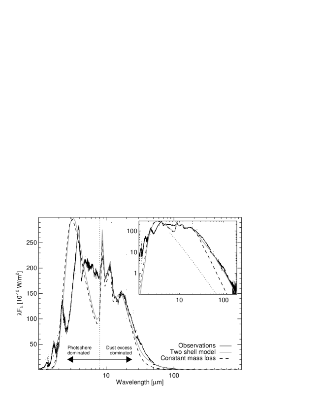
Figure 1: SED of WX Psc (black), together with the best fit dust model (gray) and the best fitting constant mass-loss rate model (dashed). The inset shows the same SEDs using logarithmic axes in order to emphasize the far-IR slope. Note that the large discrepancies between the observed and modeled SEDs between 1$-$8 $\mu$m are due to the representation of the stellar atmosphere by a blackbody. The wavelength range which is dominated by (unmodeled) photospheric features is to the left of the dotted line at 8 $\mu$m. The main absorption and emission features in the 1$-$8 $\mu$m range are due to H₂O, SiO and CO. The dust absorption and emission is best traced beyond 8 $\mu$m (see text for more details). The dotted line in the inset gives an indication of the level of the photospheric contribution to the total flux.

Table 1: Mass-loss rates for WX Psc as found in literature. Data used in this paper are indicated with the superscript ^†; the appropriate telescope diameter (in meter) and beam size (in ^′′) are listed in the last column.

Observ. data	$\dot{M}$ [$M_{\odot}$ yr-1]	Comments	Ref.	Diam. – beam
CO (1$-$0)	$1.2\times 10^{-5}$	from analytical expression	Knapp & Morris (1985)	7m – $100^{\prime\prime}$
CO (1$-$0)	$2.4\times 10^{-5}$	theor. model of Morris (1980)	Sopka et al. (1989)	20m – $42^{\prime\prime}$
CO (1$-$0)	–		Margulis et al. (1990)	14m – $45^{\prime\prime}$
CO (1$-$0)	–		Nyman et al. (1992)†	20m – $42^{\prime\prime}$
CO (1$-$0)	$8.5(\pm 2.39)\times 10^{-6}$	from analytical expression	Loup et al. (1993)
CO (1$-$0)	$1.0\times 10^{-5}$	self-consistent $T(r)$ + NLTE radiat. transfer	Justtanont et al. (1994)
CO (2$-$1)	$2.6\times 10^{-5}$	from analytical expression	Knapp et al. (1982)	10m – $30^{\prime\prime}$
CO (2$-$1)	$1.0\times 10^{-5}$	large difference between data and model	Justtanont et al. (1994)
CO (2$-$1)	$5.0\times 10^{-5}$	from analytical expression	Jura (1983)
CO (2$-$1),(3$-$2),	$0.14-8.0\times 10^{-6}$	from model Justtanont et al. (1994)	Kemper et al. (2003)†	15m – (see text)
(4$-$3),(6$-$5),(7$-$6)
L - [12$\mu$m]	$2.0\times 10^{-5}$	dust modeling	Kemper et al. (2002)
OH maser	$2\times 10^{-5}$	using Eq. (3) in Bowers et al. (1983)	Bowers et al. (1983)
$J$, $H$, $K^{\prime}$ +	$1.3-2.1\times 10^{-5}$	spherical dusty wind with	Hofmann et al. (2001)
SED + ISI (11 $\mu$m)		$\rho\propto r^{-1.5}$ from 137 $R_{\star}$ on
$J$, $H$, $K^{\prime}$ +	$1.3\times 10^{-4}$	spherical dusty wind	Tevousjan et al. (2004)
ISI (11 $\mu$m)
$J$, $H$, $K^{\prime}$ +	$9\times 10^{-6}$ last 550 yr	spherical dusty wind + cocoon	Vinković et al. (2004)
SED	$2\times 10^{-5}$, 550 – 5500  yr

The analysis is based on (i) rotational CO line profiles found in the literature and (ii) the SED in the range from 0.7 to 1300 $\mu$m. The applied CO-dataset is indicated with the superscript $\dagger$ in Table 1. Main emphasis is put on the high-quality data obtained by Kemper et al. (2003) on the 15 m JCMT telescope on Mauna Kea, Hawai. The half power beam width of the different receivers was $19.7^{\prime\prime}$ for CO (2$-$1), $13.2^{\prime\prime}$ for CO (3$-$2), $10.8^{\prime\prime}$ for CO (4$-$3), $8.0^{\prime\prime}$ for CO (6$-$5), and $6.0^{\prime\prime}$ for CO (7$-$6). The absolute flux calibration accuracy was estimated to be 10 % for the CO (2$-$1), (3$-$2) and (4$-$3), and ${\sim}$30 % for the CO (6$-$5) and (7$-$6) line because the flux standards, that are available for these higher excitation lines, are less reliable. We note that in principal pointing uncertainties, beam effects, atmospheric seeing, and systematics at these frequencies can conspire against you to produce an error that is larger than 30 %. Unfortunately we don’t have enough statistics information on standards etc. to know for sure how bad a problem this was for the RxE and RxW/D receivers at the time of the observations.

The SED of WX Psc is that of a strongly reddened Mira-type variable star with a period of 660 days and a K band amplitude of 3.4 mag (Samus et al. 2004). Two full spectral scans from both spectrometers (Short Wavelength Spectrometer (SWS) and Long Wavelength Spectrometer (LWS)) onboard the Infrared Space Observatory (ISO) satellite are available. Due to the pulsation of the star the flux levels of the SWS spectra differ by a factor $\sim$2. We opt to use the SWS spectrum taken on 15 Dec 1996 (tdt 39502217) and the LWS spectrum from 15 Jun 1997 (tdt 57701103). Although these spectra have not been obtained simultaneously, the flux levels in the overlapping region between SWS and LWS agree reasonably well because the observing dates correspond to phases 0.38 and 0.66, i.e. roughly symmetric compared to the minimum at 0.5. We have further used the 0.97$-$2.5 $\mu$m near-IR spectrum from Lançon & Wood (2000) scaled to the flux-level of the SWS spectrum. The IR spectroscopic data have been supplemented by optical and IR photometric data (Cutri et al. 2003; Dyck et al. 1974; Beichman et al. 1988; Smith et al. 2004; Morrison & Simon 1973; Hyland et al. 1972), sub-mm photometry (Sopka et al. 1989) and radio measurements (Walmsley et al. 1991; Dehaes et al. 2006) in order to construct the full SED (see Fig. 1).

In the wavelength region up to $\sim$8 $\mu$m, photospheric absorption features and emission features arising from density enhancements in the outer atmosphere caused by pulsational levitation are visible. Specifically, the CO first overtone and H₂O $\nu_{1}$ symmetric stretch and $\nu_{3}$ asymmetric stretch band features are arising between $\sim 2$ and $3.8$ $\mu$m, the small absorption peak around 4.05 $\mu$m is caused by the SiO first overtone, with the stronger absorption peak at slightly larger wavelengths (at $\sim$5 $\mu$m) mainly being due to the CO fundamental vibration-rotation band. From 6.27 $\mu$m onwards, the H₂O $\nu_{2}$ vibrational bending band is the main absorption feature. However, for the purpose of determining the mass-loss history of WX Psc, a detailed analysis of the atmospheric behaviour of this target is not a prime issue. In the framework of the dust modeling presented here, we simply represent the central star by a blackbody. The assumption of a blackbody for the underlying star does not influence the conclusions since dust emission and absorption dominates over photospheric effects beyond 8 $\mu$m (see Fig. 1). We focus on several dust characteristics of the SED and IR spectroscopy to estimate the mass loss. The most significant of these are 1) the average reddening of the star; 2) the self-absorption of the 10 $\mu$m silicate feature; 3) the relative strength of the 10 and 20 $\mu$m bands, and 4) the slope in the mid- to far-IR. These observables trace the relative amounts of dust near and further away from the star, i.e.  the columns of warm and cooler material along the line of sight.

3 Analysis

To constrain the dust-driven wind structure from its base out to several thousands of stellar radii, we use both molecular line fitting of the CO rotational $J=1-0$ through 7$-$6 line profiles and dust radiative transfer simulations of the global SED and IR spectrum. The spectral lines are modeled using GASTRoNOoM, the dust continuum using modust. We briefly discuss both programs in Sect. 3.1. Special emphasis is given on the model selection procedure and on the measure of the goodness-of-fit in Sect. 3.1.3. The results are presented in Sect. 4.

3.1 Theoretical code

3.1.1 GASTRoNOoM

The observed line profiles provide information on the thermodynamical structure of the outflow of WX Psc. For a proper interpretation of the full line profiles, we have developed a theoretical model (GASTRoNOoM - Gas Theoretical Research on Non-LTE Opacities of Molecules) which first (1) calculates the kinetic temperature in the shell by solving the equations of motion of gas and dust and the energy balance simultaneously, then (2) solves the radiative transfer equation in the co-moving frame (CMF, Mihalas et al. 1975) using the Approximate Newton-Raphson operator as developed by Schönberg & Hempe (1986) and computes the NLTE level-populations consistently, and finally (3) determines the observable line profile by ray-tracing. A full description of the code is presented in Decin et al. (2006). The main assumption is a spherically symmetric mass loss. The mass-loss rate is allowed to vary with radial distance from the star. Note that the gas and drift velocity are not changed accordingly. Adopting a value for the gas mass-loss rate, the dust-to-gas ratio is adjusted until the observed terminal velocity is obtained. For details on the thermal balance, the gas and dust velocity, and the treatment of variable mass loss we refer to Decin et al. (2006). We already note that for solving the radiative transfer equation in the CMF-frame in the case of WX Psc, we have used a value for the mass-loss rate, $\dot{M}$, equal to $1\times 10^{-5}$ $M_{\odot}$/yr.

3.1.2 MODUST

We have used the code modust (Bouwman et al. 2000) to model the transfer of radiation through the dusty outflow of WX Psc. This code has been applied extensively to model not only the dust in the outflows of supergiants and AGB stars (e.g. Voors et al. 2000; Kemper et al. 2001; Dijkstra et al. 2003; Hony et al. 2003; Dijkstra et al. 2006), but also solid state particles in proto-planetary disks and comets (e.g. Bouwman et al. 2003). In short, the code assumes a spherical distribution, such as an outflow or shell, of dust grains in radiative equilibrium that are irradiated by a central star. Here, we represent the photospheric energy distribution of WX Psc by a blackbody (see Sect. 2). A special circumstance in the modeling of WX Psc is that we account for two distinct dust shells (see Sect. 4.2). For the inner shell we do a consistent radiation transfer solution, for the outer shell we assume that the dust medium is optically thin and that it is irradiated by the light emerging from the inner shell. We have verified that indeed the outer shell of WX Psc is optically thin.

3.1.3 Parameter estimation, model selection, and the assessment of goodness-of-fit

The observational line data are subject to two kinds of uncertainties: (1) the systematic or absolute errors, with variance $\sigma^{2}_{{\rm abs}}$, arising e.g. from uncertainties in the correction for variations in the atmospheric conditions, and (2) the statistical or random errors $\varepsilon$, with variance $\sigma^{2}_{{\rm stat}}$, which reflect the variability of the points within a certain bin. Both kind of errors have to be taken into account when estimating the model parameters. In case of the CO line profiles, the statistical errors (rms) are smaller than the systematic errors. We hence will construct a statistical method giving a greater weight to the line profile than to the integrated line intensity. Moreover, as demonstrated in Decin et al. (2006), especially the line profiles yield strong diagnostics for the determination of the mass-loss history.

To determine the mass-loss history of WX Psc from the CO line profiles, a grid of ${\sim}$300 000 models was constructed. In a first step, the models for which the predicted line profiles did not fulfill the absolute-flux calibration uncertainty criterion were excluded. This absolute flux criterion does not only include the absolute flux uncertainty on the data as specified in Sect. 2, but also incorporates the noise on the data. From then on, the other models were treated equally when judging the quality of the line profile shape. To do so, a scaling factor based on the ratio of the integrated intensity of the observed data to the integrated intensity of the predicted data was introduced to re-scale the observational data. From a statistical standpoint, this scaling factor merely is an additional model parameter, accounting for the calibration uncertainties.

Assume a model for the re-scaled observed spectrum $y_{i}$ at velocity $i$, $i=1,2,\dots,n$ with expected mean value ${\rm{E}}(y_{i})=\mu_{i}$, representing the theoretical spectrum of the target. The statistical measurement errors are assumed to be normally distributed with mean 0 and variance taken to be constant at all frequency points $i$, i.e. $\sigma_{{\rm stat}_{i}}\equiv\sigma_{\rm stat}$. Hence, the model is assumed to follow a normal distribution

$$y_{i}=\mu_{i}+\varepsilon_{i},\ \ {\rm where\ }\varepsilon_{i}\sim N(0,\sigma^{2}_{\rm stat}).$$ (1)

A key tool in model selection and fitting, and in the assessment of goodness-of-fit, is the log-likelihood function which, for the normally distributed case, takes the form $\ell$, defined as:

$$\ell=\sum_{j=1}^{N_{\rm lines}}\left(\sum_{i=1}^{n_{j}}\left[-\ln(\sigma_{{\rm stat}_{j}})-\ln(\sqrt{2\pi})-\frac{1}{2}\left(\frac{y_{j,i}-\mu_{j,i}}{\sigma_{{\rm stat}_{j}}}\right)^{2}\right]\right),$$ (2)

where $N_{\rm lines}$ represents the total number of rotational lines being 6, and $n_{j}$ the number of frequency points in the $j$-th line profile (Cox & Hinkley 1990). The model which best fits the observed data maximizes the log-likelihood distribution.

Table 2: $(1-\alpha)\,100$ % quantile of the $\chi^{2}_{p}$-distribution, with $p$ degrees of freedom and a significance level $\alpha=0.05$.

$p$	$\chi^{2}_{p}(\alpha)$	$p$	$\chi^{2}_{p}(\alpha)$
1	3.8414588	11	19.675138
2	5.9914645	12	21.026070
3	7.8147279	13	22.362032
4	9.4877290	14	23.684791
5	11.070498	15	24.995790
6	12.591587	16	26.296228
7	14.067140	17	27.587112
8	15.507313	18	28.869299
9	16.918978	19	30.143527
10	18.307038	20	31.410433

One can derive three properties from the log-likehood distribution (see Welsh 1996). First, for a given parametric model, maximizing $\ell$ leads to the so-called maximum likelihood estimator $\widehat{{\mbox{\boldmath$\theta$}}}$ for the model parameters. Denote by $\ell_{m}$ the value of the log-likelihood function at maximum. Standard errors are deduced as the square root of the diagonal of the negative inverse information matrix. The information matrix is the matrix of second derivatives of the log-likelihood function w.r.t. the model parameters.

Second, the log-likelihood function can be used to determine $(1-\alpha)\,100\,\%$ confidence intervals for the model parameters, where $\alpha$ is the significance level. Precisely this is done through the method of profile likelihood, and the corresponding intervals are termed ‘profile likelihood confidence intervals’. Let us focus on one of the parameters, $\varphi$ say. The profile likelihood interval is defined as the values $\varphi$ for which $\ell_{\varphi}\equiv\ell(\varphi,\widehat{{\mbox{\boldmath$\theta$}}}(\varphi))$ is sufficiently close to $\ell_{m}$. We use $\widehat{{\mbox{\boldmath$\theta$}}}(\varphi)$ as the parameter that maximizes the log-likelihood function subject to the constraint that $\varphi$ is kept fixed. Sufficiently close is to be interpreted in the precise sense that $2(\ell_{m}-\ell_{\varphi})\leq\chi^{2}_{1}(\alpha)$, where $\chi^{2}_{1}(\alpha)$ is the $(1-\alpha)\,100\%$ quantile of the $\chi^{2}_{1}$ distribution. The same procedure can be used for a group of $p$ parameters simultaneously. In this case $\varphi$ is $p$-dimensional and the quantile is now of the $\chi^{2}_{p}(\alpha)$-distribution (see Table 2). In our case, the confidence intervals are influenced by the grid spacing, but they converge to the true intervals if the grid spacing becomes arbitrarily fine.

Third, the log-likelihood function can be used to compare two different models, with a different number of parameters, $p$ and $p+r$, as long as they are nested. The more elaborate model is preferred if $2(\ell^{p+r}_{m}-\ell^{p}_{m})\geq\chi^{2}_{r}(\alpha)$, otherwise preference points towards the simpler model.

One should realize that the outlined log-likelihood method does not force the accordance between observations and predictions to be better than a certain pre-specified level in order to be acceptable. This is in contrast with the often used reduced-$\chi^{2}$-method, which requires that for a good fit the value of the reduced-$\chi^{2}$ should be lower than 1 (or 2). Using the log-likelihood method, one is selecting the theoretical predictions (and corresponding confidence intervals for the model parameters) with the best fit to the data in the framework of the applied theoretical model.

As an example, we describe the selection of the best model and the determination of the 95 % confidence intervals of the stellar and mass-loss parameters as derived from the CO line fitting procedure (see Sect. 4.1). In Fig. 2 an example is shown of a mass-loss profile with 4 $\dot{M}$-phases and 3 small interfaces (each described by 2 parameters ($R_{i}$, $\dot{M}$_i)). This mass-loss profile is hence described by 6 pairs ($R_{i}$, $\dot{M}$_i), indicated with diamonds in Fig. 2. Other free parameters in the grid computation were the stellar temperature $T_{\star}$, dust condensation radius $R_{\rm{inner}}$, and outer radius of the CSE $R_{\rm{outer}}$, resulting in 15 free parameters in total. We note that for the modelling of WX Psc the value of $\dot{M}$ at $R_{\rm{inner}}$ was specified to stay constant till the first decrease in mass loss at $\sim$30 $R_{\star}$, and also from 1550 $R_{\star}$ on the mass-loss was kept constant until $R_{\rm{outer}}$. This is however not a prerequisite to the code, but has been introduced to reduce the grid computations. Our best-fitting model has a log-likelihood $\ell_{m}=-314.17$. The 95 % confidence intervals are determined by all models whose log-likelihood $\ell$ is $2(\ell_{m}-\ell)\leq\chi^{2}_{15}(\alpha)$, i.e. $2(\ell_{m}-\ell)\leq 24.99579$ or $-326.6\leq\ell\leq-314.17$. If we want to test if a model with 3 episodes of high mass loss yields a significantly better result than with 2 high-mass epochs, we are introducing 4 extra pairs ($R_{i}$, $\dot{M}$_i), i.e. 8 free parameters. Hence, the more elaborate model with 23 parameters is preferred when the maximum of the log-likelihood of the 3-shell model ($\ell_{m}^{23}$) obeys $2(\ell^{23}_{m}-\ell^{15}_{m})\geq\chi^{2}_{8}(\alpha)$ or $\ell_{m}^{23}\geq-306.41$.

4 Results

4.1 Modeling the CO rotational line profiles

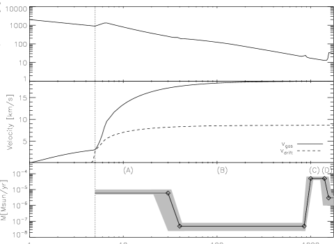
Figure 2: Upper: Estimated temperature profile, middle: estimated velocity structure, and bottom: estimated mass-loss rate $\dot{M}$$(r)$ for WX Psc as a function of radial distance to the star (black line). The shading region in the bottom panel displays the confidence intervals of the estimated mass-loss parameters.

Table 3: Parameters of the model with best goodness-of-fit for WX Psc. In the second column models parameters as derived from the CO rotational lines are listed, in the third column the parameters as estimated from the SED fitting are given. The numbers in italics are input parameters that have been kept fixed at the given values. There is, of course, an interdependence between $T_{\star}$, $R_{\star}$ and $L_{\star}$ and between $L_{\star}$, the distance, and $m_{bol}$ from which the distance has been derived.

parameter	from CO lines	from SED fitting
$T_{\star}$ [K]	2000	2000
$R_{\star}$ [$10^{13}$ cm]	5.5	5.5
$L_{\star}$ [$10^{4}$ $L_{\odot}$]	1	1
dust-to-gas ratio	0.004	0.004
$\varepsilon$(C) [$10^{-4}$]	3	$-$
$\varepsilon$(O) [$10^{-4}$]	8.5	$-$
distance [pc]	833	833
$R_{\rm{inner}}$ [$R_{\star}$]	5	5
$R_{\rm{outer}}$ [$R_{\star}$]	1750	1500†
$v_{\infty}$ [km s-1]	18	18
$\dot{M}$$(r)$ [$M_{\odot}$yr-1]   (A)	${\sim}6\,10^{-6}$ ($\sim$5$-$30 $R_{\star}$)	${\sim}4\,10^{-5}$ ($\sim$5$-$50 $R_{\star}$)
$\dot{M}$$(r)$ [$M_{\odot}$yr-1]   (B)	${\sim}5\,10^{-8}$ ($\sim$30$-$850 $R_{\star}$)	$-$
$\dot{M}$$(r)$ [$M_{\odot}$yr-1]    (C)	${\sim}5\,10^{-5}$ ($\sim$850$-$1450 $R_{\star}$)	${\sim}3\,10^{-4}$ ($\sim$800$-$1500 $R_{\star}$)
$\dot{M}$$(r)$ [$M_{\odot}$yr-1]    (D)	${\sim}3\,10^{-6}$ ($\sim$1450$-$1750 $R_{\star}$)	$-$

^† The outer radius mentioned in the SED fitting refers to the outer edge of the second shell, called region (C) in Fig. 2, and should be compared to the 1450 $R_{\star}$ value derived from the CO modeling.

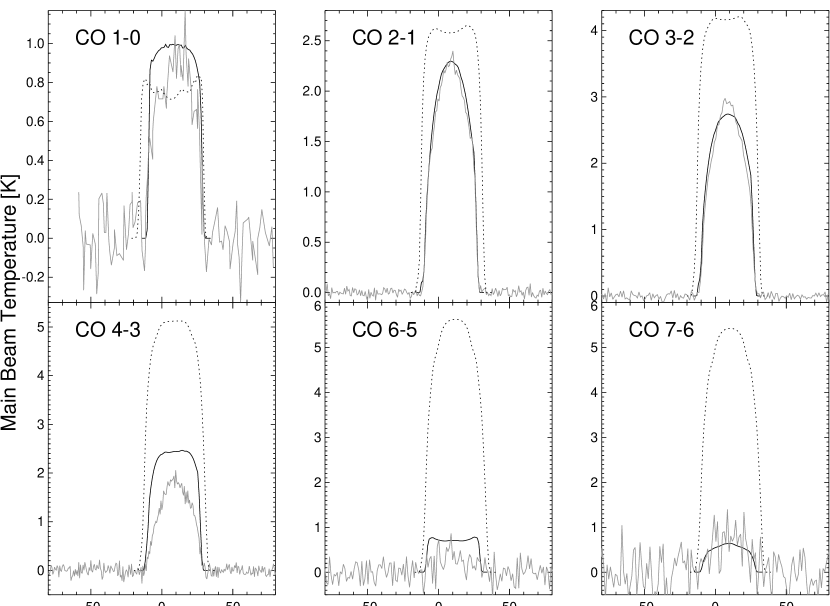
Figure 3: CO rotational line profiles of WX Psc (full grey line; Nyman et al. 1992; Kemper et al. 2003) compared with (i) black dotted line: the model predictions based on the parameters as given by Justtanont et al. (1994), who assumed a constant mass loss of $\dot{M}$ = $1\times 10^{-5}$ $M_{\odot}$ yr^-1 and a distance of 850 pc, and (ii) full black line: the best-fit model with parameters as specified in Table 3.

Comparing the observed CO line profiles with theoretical profiles predicted by a model assuming a constant mass loss confirms the hypothesis proposed by Kemper et al. (2003) that variable mass loss may play an important role in the shaping of the spectral line profiles (see dotted line in Fig. 3).

Using the procedure as outlined in Sect 3.1.3, a total amount of ${\sim}$300 000 models was run to estimate the mass-loss history of WX Psc. A luminosity of $1\times 10^{4}$ $L_{\odot}$ was assumed, which together with the integrated luminosity of the SED yields a distance of 833 pc. The expansion velocity traced by all line profiles is $v_{\infty}=18\pm 1$ km s^-1. For the carbon and oxygen abundances in the outer atmosphere of the target, we opt to use the cosmic abundance values of Anders & Grevesse (1989, see Table 3), and it is assumed that in case of the oxygen-rich target WX Psc all of the available carbon will be locked in CO. Other model parameters as stellar temperature $T_{\star}$ (or stellar radius $R_{\star}$), dust condensation radius $R_{\rm inner}$, outer radius of the envelope $R_{\rm outer}$ and the mass-loss profile were kept free in the grid running. In case of constant mass loss, the value of $R_{\rm outer}$ is set at the radius where the CO abundance drops to 1 % of its value at the photosphere, using the photodissociation results of Mamon et al. (1988) (see Decin et al. 2006). However, the CO photodissociation radius by Mamon et al. (1988) were obtained in case of constant mass loss, and it is questionable how this applies when dealing with variable mass loss. In case of variations in the mass loss, we therefore opt to have $R_{\rm outer}$ as free parameter, with the additional constraint that $R_{\rm outer}$ should be smaller than the $R_{\rm outer}$-value obtained using the formula of Mamon et al. (1988) for a value of the mass loss equal to the mass-loss rate at the outermost radius point. We hereby want to ensure not to go beyong the photodissociation radius as calculated by Mamon et al. (1988). Moreover, it is always checked that the full line forming region (as traced by $I(p)\times p^{3}$, see e.g. Fig. 5 and 6 in Decin et al. 2006) of all rotational CO lines lies within $R_{\rm{outer}}$.

Parameters characterizing the CSE of the model with the best goodness-of-fit are specified in the second column of Table 3. The derived temperature profile, velocity structure and mass-loss history are displayed in Fig. 2; a comparison between observed and theoretical line profiles is shown in Fig. 3. We note that the abruptness of changes in the mass-loss profile causes the small-scale ripples seen in the CO line profiles. The presence of the noise in the line profile does however not influence the conclusions in this paper. The dust-to-gas ratio is derived from the mass-loss rate and terminal velocity and equals 0.004. This value for the dust-to-gas ratio is quite uncertain. As described in Decin et al. (2006), this value is taken constant throughout the entire envelope. However, a higher mass-loss rate as in region (C) can drive a dusty wind with a different velocity than in a low-mass region and perhaps also with a different dust-to-gas ratio. In this respect, we note that the different CO lines, originating from various parts in the wind, do not exhibit different line widths (Fig. 3).

Before comparing with the results of the SED fitting (Sect. 4.2), we first discuss the derived $\dot{M}$-profile and associated uncertainties (see bottom panel in Fig. 2). Acceptable values for the mass-loss rate in region (A) range from $5\times 10^{-6}$ to $1\times 10^{-5}$ $M_{\odot}$ yr^-1, for region (B) from $2.5\times 10^{-8}$ to $8\times 10^{-8}$ $M_{\odot}$ yr^-1, for region (C) from $4\times 10^{-5}$ to $6.5\times 10^{-5}$ $M_{\odot}$ yr^-1, and for region (D) from $1\times 10^{-6}$ to $4\times 10^{-6}$ $M_{\odot}$ yr^-1. Especially region (C) with enhanced mass loss is constrained quite well since the (high-quality) low-excitation lines are mainly formed in this region. Notice that the temperature increase in region D (see top panel in Fig. 2) is quite uncertain: an altered temperature structure with a continuously decreasing temperature reaching 10 K at the outer radius, yields line intensity profiles which are better for all low-excitation transitions, and has a log-likelihood that is significantly better than that of our ‘best-fit’ model with an amount $\Delta\ell=105$. The main cause of uncertainty in $T(r)$ is that interactions between the different shells and with the ISM are not taken into account.

Inspecting Fig. 3, we see a good resemblance between the observations and model predictions for the CO (1–0), (2–1) and (3–2) lines. The predicted peak intensity of the CO (4–3) and (6–5) line is somewhat too high. This may indicate that the temperature in region C, where the dominant part of these lines is formed, may be somewhat lower than is inferred.

Almost half of the models was run with a third shell extending between $\sim$100 and $\sim$600 $R_{\star}$, and with mass-loss rates ranging between $2\times 10^{-8}$ and $3\times 10^{-5}$ $M_{\odot}$ yr^-1. The model with the best fit had $\dot{M}$ = $5\times 10^{-8}$ $M_{\odot}$ yr^-1 both in region (B) and in this extra third shell, i.e. the statistical analysis gives preference to a 2-shell model above a 3-shell model. Models still having an acceptable fit to the line profiles, all had $\dot{M}$ $\leq 2.5\times 10^{-7}$ $M_{\odot}$ yr^-1 in this third shell.

4.2 SED fitting

The SED of the best fitting model is presented in Fig. 1 and the implied model parameters are given in Table 3. As described above, the model consists of two shells that present two episodes of high mass loss. The intermediate period of significantly lower mass loss is not modeled. In general, we find that the wind structure that best reproduces the observed SED has very similar parameters to those derived from modeling the CO rotational lines. In particular, the two methods agree on the location of the inner edges of the two shells. The outer radii of the shells can be chosen to be roughly consistent with the values derived from the molecular modeling. It is impossible to derive statistical uncertainties on the derived parameters since the best fitted model is not obtained through a formal fitting procedure (like was done for the CO lines). Such a formal fitting procedure is inhibited by the very unequal weighting that is given to the various regions of the SED. For example, the region which is dominated by water vapour emission and absorption is virtually neglected. While the integrated photospheric component is used as a constraint, no single optical wavelength range is given priority. In contrast the 8 – 25 $\mu$m range, which exhibits the clearest dust spectral signatures, is inspected in detail. Furthermore, the IR-submm slope is used as a strong constraint eventhough it is determined by far fewer points than the mid-IR part. However we can determine by how much we can vary the parameters without significantly reducing the quality if the fit. Varying, e.g., the inner radii of the two shell model by $\sim$10 per cent, significantly degrades the quality of the fit. We also note that the dust model results are less sensitive to the precise extent of the dust shell than to the amount of mass contained in the shell. Therefore, the outer radii are less well constrained. An important conclusion that can be drawn is that the self-absorption and relative strengths of the 10 and 20 $\mu$m silicate features arise from a dense and compact shell close to the photosphere. To illustrate this point we also show in Fig. 1 the “best” fitting model using a single shell from a constant mass loss ($\dot{M}$= 1.5 10^-5 M_⊙; $R$=5$-$200 R_⊙). A more extended shell would yield too much cold dust and a less dense wind would not yield enough self-absorption. This compact shell is however not sufficient to explain the far-IR data. The slope of the SED in the far-IR is dominated by cool material (see inset in Fig. 1).

4.3 CO versus SED fitting

The fact that these very different tracers yield such similar parameters with respect to the location of the densest shells is remarkable and builds further confidence in the reality of the mass-loss variabilities. However, it should be noted that the mass-loss rates derived from fitting the SED (column 3 in Table 3) are higher than those found from modeling the CO emission (column 2 in Table 3), by roughly a factor 6. Partly, the discrepancy can be accounted for by considering the material contained in the regions that are not included in the dust model (B and D). Some experimenting with the dust modeling shows that the differences can not be reconciled by adapting the dust composition alone. Upon perusal of Table 1, it appears that those studies that take the thermal IR emission into account systematically derive a denser wind than those using gas tracers alone. The difference may be related to the assumed CO/H₂ ratio (see Table 3). Under the assumption that all carbon is locked in CO, the CO/H₂-ratio used in this paper is $3\,10^{-4}$. Zuckerman & Dyck (1986) used a value of $5\,10^{-4}$ for the CO/H₂-ratio in O-rich giants, while Knapp & Morris (1985) reported a value of $3\,10^{-4}$. This value differs from AGB star to AGB star, as it is dependent on the amount of dredge-up. We estimate the uncertainty on the used CO/H₂-ratio to be a factor 2. In addition, as described in Sect. 4.1, the derived dust-to-gas ratio as calculated from the CO modeling is somewhat uncertain. This value is not only taken constant throughout the whole envelope, but moreover it is assumed that all the dust particles participate in accelerating the wind to the observed outflow velocity. The discrepancy in dust content between the two types of models may signify that a sizable fraction of the dust, though present, does not contribute much to the acceleration of the wind. If some fraction of the dust particles is effectively shielded from illumination by the star, they will not feel the radiation force from the star and, by consequence, will not contribute to the acceleration of the wind. This kind of shielding can typically occur in randomly distributed density inhomogeneities (usually referred to as clumps) or can be due to deviations of spherical symmetry. Only some fraction of the dust is hence responsible for the driving; via collisions with the inert gas, the gas is accelerated, which in it turn may accelerate the inert dust. In the acceleration of the gas particles, it is not only assumed that all dust particles participate in this proces, but also that the dust grains transfer all of the momentum they acquire from the radiation field to the gas through collisions. Therefore, an alternative explanation could be that there is an incomplete momentum coupling between the dust and the gas in the wind (e.g. MacGregor & Stencel 1992). Lastly, an explanation could have been dust which is not partaking in the outflow but present in a stable configuration, i.e. a disk. However, the gaseous material present in such a slowly rotating disk would be detected via the presence of a very narrow line profile (typically line width less than 5 km s^-1) superimposed on a broad outflow component (e.g. as is the case of RV Boo, Bergman et al. 2000). Since such a narrow component is not detected in any of the line profiles this explanation is ruled out.

5 Discussion

The diagnostic power of estimating the mass-loss history from modeling the rotational CO line profiles and the full SED, is evident. Both our CO and SED modeling are however based on one common assumption, namely a spherically symmetric envelope. We comment on this assumption in Sect. 5.1. In Sect. 5.2 we compare our results to other studies. We discuss the time scale of the mass-loss variability and its implication on the possible mechanism driving this variability in Sect. 5.3.

5.1 Structure of the circumstellar envelope

The detailed structure of the CSEs of AGB stars and the physics driving this structure remain unknown after half a century of study. The main reason being that the cool material is a real challenge to high-resolution observations. From a survey of AGB envelopes using millimeter interferometry, Neri et al. (1998) concluded that most (${\sim}$70 %) AGB envelopes are consistent with spherical symmetry. WX Psc belongs to the small group of AGB stars whose CSE has already been studied using different techniques, and for which several indications are found for deviations from a spherically symmetric envelope. (1) Neri et al. (1998) fitted the CO (1–0) and (2–1) interferometric observations with a two-component Gaussian visibility profile consisting of a circular and an elliptical component. The circular flux-dominant component corresponds to a spherical envelope with a $29^{\prime\prime}.6$ diameter, the elliptical one to an axisymmetric envelope with major axis of $9^{\prime\prime}.8$ and minor axis of $6^{\prime\prime}.8$, and a position angle of $-45^{\circ}$ (E to N). (2) Broad-band near-infrared polarimetry performed by McCall & Hough (1980) revealed that WX Psc is highly polarized in the $I$ and $J$-band, while the polarization pattern is not dominant in the $H$ and $K^{\prime}$-band. This may either indicate an alignment of dust particles or an asymmetrical dust-shell structure. (3) Another technique of imaging the circumstellar dust is from bispectrum speckle-interferometry. Using this technique, Hofmann et al. (2001) showed that the $H$ and $K^{\prime}$-band images of WX Psc appear almost spherically symmetric, while the $J$-band shows a clear asymmetry. Two structures can be identified in the $J$-band image: a compact elliptical core and a fainter fan-like structure, along a symmetry axis of position angle $-28^{\circ}$, out to distances of ${\sim}$200 mas. (4) Mauron & Huggins (2006) imaged the circumstellar dust in scattered light at optical wavelengths. While the images of the extended envelope appear approximately circularly symmetric in the $V$-band, the Hubble Space Telescope (HST) images revealed that the inner region of the CSE consists of a faint circular arc at ${\sim}$0.8″to the NW and a highly asymmetric core structure, with a bright extension out to ${\sim}$0.4″(or 90 $R_{\star}$ at 833 pc) at position angle $-45^{\circ}$. Most likely, the HST image captures the extension of the core asymmetry seen in the $J$-band. They concluded that WX Psc is somewhat similar to IRC +10216 where approximate circular symmetry and shells in the extended CSE co-exist with a strong axial symmetry close to the star.

Nevertheless, we assume a spherically symmetric geometry for the whole wind structure when modeling the SED and CO line profiles. The different direct pieces of evidence for deviation of spherical symmetry all trace small scales ($\la 200$ mas). On larger scales, the shell does not appear to deviate significantly from spherical symmetry. Note that the beam profiles used in the CO observations are larger than $6^{\prime\prime}$, and thus measure the temperature, density and velocity averaged in all directions in the regions where the lines are mainly formed. Hence, the main stellar and mass-loss properties can be inferred from spherically symmetric models in fair approximation. In reality, these average properties are formed from a superposition of all these structures in this region.

5.2 Comparison with other studies

In Sect. 5.2.1, we compare our results with mass-loss parameters obtained in previous studies also tracing the mass-loss variability of WX Psc. In Sect. 5.2.2, we focus on the $V$, $J$, $H$, and $K^{\prime}$ images of Mauron & Huggins (2006) and Hofmann et al. (2001) probing both the dust-scattered stellar and galactic light and the thermal dust emission.

5.2.1 Mass-loss parameters

Hofmann et al. (2001) modeled the SED between 1 $\mu$m and 1 mm, together with the visibility functions at 1.24 ($J$ band), 1.65 ($H$), 2.12 ($K^{\prime}$) and 11 $\mu$m using dusty (Ivezić et al. 1997). The visibility data provide information on the innermost regions of the circumstellar environment, probing the scattering properties of the dust (at $J$) and thermal emission properties of the hot and warm dust (at $H$, $K$ and 11 $\mu$m). Assuming a spherical outflow, they found that both the near-IR visibilities as well as the mid-IR photometric points up to 100 $\mu$m could be well reproduced by a two-component outflow in which dust condenses at 900 K. The most recent mass loss, characterized by a constant velocity outflow (i.e. $\rho\propto r^{-2}$), is $\hbox{$\dot{M}$}\,=\,1.3-2.1\times 10^{-5}$ $M_{\odot}$ yr^-1. At distances beyond 135 $R_{\star}$ the density decrease is shallower, matching $\rho\sim r^{-1.5}$ (see the dashed black line in Fig. 4). At wavelengths beyond about 400 $\mu$m this model underestimates the observed flux.

The $J$-band data reveal an asymmetry, and the $H$-band visibility shows a puzzling drop in the $H$-band at spatial frequencies $\ga 14$ cycles per arcsec, corresponding to structure smaller than the condensation radius. The spherical model of Hofmann et al. (2001) can not address these observations. The above issues were taken up by Vinković et al. (2004). They explain the image asymmetries as originating from about 10^-4 $M_{\odot}$ of wind material that is swept-up in an elongated cocoon whose expansion is driven by bipolar jets and which extends out to a radial distance of ${\sim}$1100 AU (or 300 $R_{\star}$), with an opening angle of ${\sim}$30^∘. The two cocoons have a characteristic lifetime that is $\la 200$ yr. To explain the mid-IR spectrum they invoke a spherical envelope (in which the cocoons are embedded) containing ${\sim}$0.13 $M_{\odot}$ of material extending out to ${\sim}$35″ (or $\sim$8 000 $R_{\star}$). The size of the envelope corresponds to a dynamical flow time of 5 500 yr. Over time the mass loss rate has decreased. While $\hbox{$\dot{M}$}\sim 2\times 10^{-5}$ $M_{\odot}$ yr^-1 until 550 yr ago, the most recent mass-loss is estimated to be only ${\sim}$9$\times 10^{-6}$ $M_{\odot}$ yr^-1. Two-dimensional radiative transfer calculations demonstrate that this model can explain both the $J$-band asymmetry, being dominated by scattered light escaping through the cone, and the spherical symmetry seen in the $H$ and $K^{\prime}$-band images, being due to predominantly thermal dust emission. This model also fits the general structure of the SED quite well, but has some problems in explaining the silicate feature around $10$ $\mu$m and the photometric data at $\lambda>100\,\mu$m.

In general, the mass-loss rate in the spherical envelope derived by Hofmann et al. (2001) and Vinković et al. (2004) is much larger than what is implied by the CO lines (see Fig. 4) and is not consistent with the observed CO rotational line profiles (see Fig. 5). The CO (1$-$0) through (7$-$6) lines are a sensitive probe of a geometrically extended part of the CSE, save for the innermost region. This again may indicate that part of the dust does not participate in driving the wind.

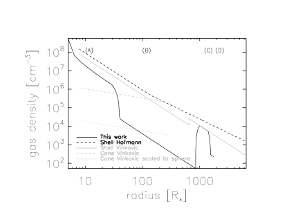
Figure 4: Number densities as a function of radial distance from the star as deduced by different authors. Full black line: spherical CSE of this study; dashed black line: spherical CSE of Hofmann et al. (2001); full grey line: spherical CSE of Vinković et al. (2004); dashed grey line: bipolar cone of Vinković et al. (2004); dotted grey line: number density of bipolar cone of Vinković et al. (2004) scaled to a sphere.

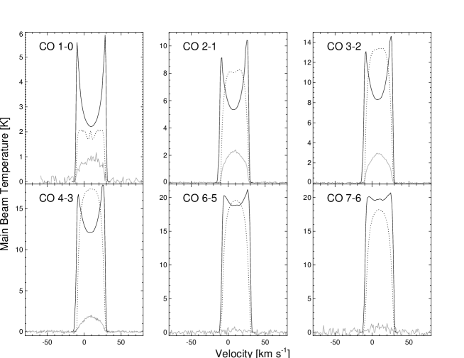
Figure 5: CO rotational line profiles of WX Psc (full grey line; Nyman et al. 1992; Kemper et al. 2003) compared with model predictions based on the parameters as proposed by Hofmann et al. (2001) (dotted black line) and Vinković et al. (2004) (full black line).

5.2.2 Dust scattered light

Besides the work by Hofmann et al. (2001) and Vinković et al. (2004), HST observations by Mauron & Huggins (2006) also trace mass-loss variability in the ambient environment of WX Psc. The HST-image shows part of a faint circular arc at ${\sim}$0.8″(or ${\sim}$180 $R_{\star}$) from the center. We performed additional simulations introducing a third shell, positioned at this location (see Sect. 4.1). These simulations demonstrate that it may be possible that a faint arc is present with a mass-loss rate $\la 2.5\times 10^{-7}$ $M_{\odot}$ yr^-1, although the log-likelihood of this more sophisticated model is not significantly better than for the simpler two-shell model. The presently available rotational CO line profiles can hence not be used to draw any conclusions on the presence of this faint arc.

Mauron & Huggins (2006) have obtained the $B$ and $V$-band scattered light profiles of WX Psc. The scattered light is predominantly due to external illumination of the shell. These images show a relatively smooth decrease of intensity as a function of distance and at face-value do not seem to necessitate the invocation of mass-loss variability to explain them. However, the observed scattered light profile is very sensitive to the location of the external illumination sources and the phase function of scatterers. Formally the expression that these authors have used to fit to the observed profiles under the assumption of uniform illuminations is incorrect. The expression that they apply concerns the scattered part of the observed intensity, while under uniform illumination this part exactly compensates the intensity which is scattered out of the beam. It is at present unclear how a variable mass-loss history would translate into an observed intensity profile on the sky as a function of these parameters. It is obvious that a forward peaked scattering function will tend to de-emphasise any mass-loss variations at large distances. But whether this effect is sufficient to explain the smooth brightness distribution remains to be seen. A proper model for the light scattering in the CSE of WX Psc, taking into account its position in the galaxy, should be constructed. This, however, is clearly beyond the scope of this paper.

5.2.3 Conclusion

To conclude, we use constraints from the dust and the CO molecules in the shell to determine the density profile within the few to few thousand stellar radii regime. The tracers we use are sensitive to these scales in a series of overlapping distance steps. The real power of our modeling comes from using both the spectral information and the absolute strength of the observed quantities, be-it the molecular lines or the dust excess. These are all explained to satisfactory detail by the model presented here. The limitations of the method are also clear. While this yields good estimates for the average density as a function of distance, neither the large-beam observations nor the spherical model have the power to draw conclusion about small-scale ($\Delta R/R\approx 0.5)$ structures or asymmetries.

5.3 Mass-loss variability

As already noted in Sect. 5.1, Mauron & Huggins (2006) concluded that WX Psc resembles IRC +10216 where approximate circular symmetry and discrete shells exist in the extended envelope. In case of IRC +10216, the shell spacing varies between 200 and 800 yr, although intervals as short as 40 yr are seen close to the star (Mauron & Huggins 2000). The time spacing between shell (A) and (C) in WX Psc is $\sim$800 yr. The total envelope mass is estimated to be 0.03 $M_{\odot}$, of which $\sim$95 % is located in region (C). Assuming WX Psc to be a typical (solar-type) AGB star losing some 0.5 $M_{\odot}$ during its AGB evolution lasting some 100 000 yr, WX Psc has already lost $\sim$6 % of the total mass that it will shed in its AGB-phase in a period of 600 yr (region C). Such a strong ejection event may indicate that WX Psc is currently in its superwind phase. Assuming that a typical oxygen-rich AGB star expels 0.1 $M_{\odot}$ during the last 1000 yr that it experiences a superwind mass-loss phase (Marigo & Girardi 2007), few such high mass-loss phases may occur during the superwind phase of WX Psc.

Various models have been proposed for the origin of discrete shells in CSEs. One type of models is based on the effects of a binary companion (see, e.g., Harpaz et al. 1997; Mastrodemos & Morris 1999). A different scenario is invoked by Simis et al. (2001), who suggested that such shells are formed by a hydrodynamical oscillation due to instabilities in the gas-dust coupling in the CSE while the star is on the AGB. Soker (2000) invoked another mechanism, being a solar-like magnetic activity cycle in the progenitor AGB star. Soker (2006) raised the possibility that semi-periodic oscillations in the photospheric molecular opacity may be another candidate mechanism for the formation of multiple semi-periodic arcs.

6 Conclusions

In this paper, we have analyzed the rotational CO (1$-$0) through (7$-$6) line profiles of WX Psc in combination with the dust characteristics in the full SED from 0.7 to 1300 $\mu$m. This combined analysis yields strong constraints on the density and temperature structure over a geometrically large extent of the circumstellar envelope, save for the innermost region. Both CO line fitting and dust modeling evidence strong mass-loss modulations during the last 1700 yr. Particularly, WX Psc underwent a high mass-loss phase ($\dot{M}$$\sim 5\,10^{-5}$ $M_{\odot}$/yr) lasting some $600$ yr and ending $\sim$800 yr ago. This period of high mass loss was followed by a long period of low mass loss ($\dot{M}$$\sim 5\,10^{-8}$ $M_{\odot}$/yr). The current mass loss is estimated to be $\sim 6\,10^{-6}$ $M_{\odot}$/yr. We want to emphasize that the time spacing of these mass loss modulations are independently well constrained by both the molecular gas and dust modeling. The uncertainty on the mass-loss rate in the different phases is estimated to be a factor of a few, mainly caused by the uncertainty on the dust-to-gas ratio and the CO/H₂ ratio, and by the assumption of a homogeneous spherically symmetric envelope. Most importantly, the mass-loss history that we derive is significantly different from a constant mass-loss rate model, and moreover implies that WX Psc can have at maximum in the order of a few high mass-loss phases during its final superwind evolution on the AGB.