Constructing presentations of subgroups of right-angled Artin groups

Abstract.

Let $G$ be the right-angled Artin group associated to the flag complex $\Sigma$ and let $\pi:G\to\mathbf{Z}$ be its canonical height function. We investigate the presentation theory of the groups $\Gamma_{n}=\pi^{-1}(n\mathbf{Z})$ and construct an algorithm that, given $n$ and $\Sigma$, outputs a presentation of optimal deficiency on a minimal generating set, provided $\Sigma$ is triangle-free; the deficiency tends to infinity as $n\to\infty$ if and only if the corresponding Bestvina–Brady kernel $\bigcap_{n}\Gamma_{n}$ is not finitely presented, and the algorithm detects whether this is the case. We explain why there cannot exist an algorithm that constructs finite presentations with these properties in the absence of the triangle-free hypothesis. We explore what is possible in the general case, describing how to use the configuration of $2$-simplices in $\Sigma$ to simplify presentations and giving conditions on $\Sigma$ that ensure that the deficiency goes to infinity with $n$. We also prove, for general $\Sigma$, that the abelianized deficiency of $\Gamma_{n}$ tends to infinity if and only if $\Sigma$ is $1$-acyclic, and discuss connections with the relation gap problem.

1. Introduction

Right-angled Artin groups, or graph groups as they used to be known, have been the object of considerable study in recent years, and a good picture of their properties has been built up through the work of many different researchers. For example, from S. Humphries [10] one knows that right-angled Artin groups are linear; their integral cohomology rings were computed early on by K. Kim and F. Roush [12], and C. Jensen and J. Meier [11] have extended this to include cohomology with group ring coefficients. More recently, S. Papadima and A. Suciu [16] have computed the lower central series, Chen groups and resonance varieties of these groups, while R. Charney, J. Crisp and K. Vogtmann [7] have explored their automorphism groups (in the triangle-free case) and M. Bestvina, B. Kleiner and M. Sageev [2] their rigidity properties.

However, the feature of these groups that has undoubtedly been the most significant in fuelling interest in them is their rich geometry. In [8], R. Charney and M. Davis construct for each right-angled Artin group an Eilenberg–Mac Lane space which is a compact, non-positively curved, piecewise-Euclidean cube complex. This invitation to apply geometric methods to the study of right-angled Artin groups was taken up with remarkable effect by M. Bestvina and N. Brady [1].

One can parametrize right-angled Artin groups by finite simplicial complexes $\Sigma$ satisfying a certain flag condition. The Artin group associated to $\Sigma$ depends heavily on the combinatorial structure of $\Sigma$, not just its topology. However, each right-angled Artin group has a canonical map onto $\mathbf{Z}$, and if one passes to the kernel of this map then Bestvina and Brady show that the cohomological finiteness properties of such a kernel are determined by the topology of $\Sigma$ alone. (See $\S$ 2 for a precise statement.)

In low dimensions, the cohomological properties of a group are intimately connected to its presentation theory, so one might hope to see directly how presentations of these Bestvina–Brady kernels are related to the corresponding flag complex $\Sigma$. This point of view was adopted by W. Dicks and I. Leary in [9]; we embrace and extend it here.

To prove their theorem, Bestvina and Brady use global geometric methods. Our aim is to understand the behaviour of subgroups of right-angled Artin groups at a more primitive, algorithmic level. Our main focus will be the algorithmic construction of finite presentations for certain approximations to the Bestvina–Brady kernels. It turns out that there are profound reasons why such an approach can only take one so far, and so philosophically one can conclude that some extra input (for example, from geometry) is essential for a complete understanding of these groups: see $\S$ 6.

Let us now describe our results. Fix a connected finite flag complex $\Sigma$. The principal objects of study in this paper are finite-index subgroups of the corresponding right-angled Artin group $G=G_{\Sigma}$ that interpolate between the well-understood group $G$ and the often badly-behaved Bestvina–Brady kernel $H=H_{\Sigma}$. Specifically, if $\pi:G\to\mathbf{Z}$ is the canonical surjection (see $\S$ 2), so that $H=\ker\pi$, then we consider the groups $\Gamma_{n}=\pi^{-1}(n\mathbf{Z})$: thus $G=H\rtimes\mathbf{Z}$ and $\Gamma_{n}=H\rtimes n\mathbf{Z}$.

Our expectation that these groups should have interesting presentation theories comes from the Bestvina–Brady theorem. Recall that the finiteness property $\mathrm{FP}_{2}$ has sometimes been called almost finite presentability in the literature, because a group $\Gamma$ enjoys this property if and only if it has a presentation $F/R$ with $F$ a finitely generated free group and the abelian group $R/[R,R]$ finitely generated as a module over the group ring $\mathbf{Z}\Gamma$, where the $\Gamma$-action is induced by the conjugation action of $F$ on $R$. This $\mathbf{Z}\Gamma$-module is called the relation module of the presentation. For a long time it was an open question whether or not almost finite presentability is in fact equivalent to finite presentability, but one part of Bestvina and Brady’s result implies that this question has a negative answer: specifically, when $\Sigma$ is a flag complex with non-trivial perfect fundamental group, they show that the kernel $H_{\Sigma}$ is almost finitely presented but not finitely presented.

Motivated by this, we investigate the extent to which the topology of $\Sigma$ determines whether or not the number of relations needed to present $\Gamma_{n}$ remains bounded as $n$ increases, and similarly whether the number of generators needed for the relation modules remains bounded. A natural conjecture is that the number of relations required remains bounded if and only if $H_{\Sigma}$ is finitely presented, while the rank of the relation module remains bounded if and only if $H_{\Sigma}$ is almost finitely presented. We prove the second part of this conjecture in this paper. In the light of this, a proof of the first part (which eludes us) would establish the existence of a finitely presented group with a relation gap, without giving an explicit example. (See [5] for a fuller discussion of the relation gap problem.)

Here is a summary of our results.

Proposition A (Proposition 4.4).

If $\Sigma$ is connected then for each integer $n\geq 1$ there is a generating set for $\Gamma_{n}$ indexed by the vertices of $\Sigma$, and $\Gamma_{n}$ cannot be generated by fewer elements.

The next two theorems are most cleanly phrased in the language of efficiency and deficiency: see $\S$ 3.

Theorem B (Theorems 4.5 and 5.1).

Suppose that $\Sigma$ is triangle-free. Then for each choice of a maximal tree in $\Sigma$ and for each integer $n$, there is an algorithm that produces an explicit presentation for $\Gamma_{n}$ with $N$ generators and $N-1+n(1-\chi(\Sigma))$ relations, where $N$ is the size of the vertex set of $\Sigma$. Moreover, these presentations are efficient.

Corollary C (Corollary 4.7).

If $\Sigma$ is triangle-free, then $\operatorname{def}(\Gamma_{n})\to\infty$ as $n\to\infty$ if and only if $H_{\Sigma}=\bigcap_{n}\Gamma_{n}$ is not finitely presentable.

The next theorem shows that there is a logical obstruction to extending Corollary C to the case when $\Sigma$ is higher-dimensional, at least using constructive methods.

Theorem D (Theorem 6.2).

Suppose there is an algorithm that generates a finite presentation $\big{\langle}A(\Sigma)\;{\big{|}}\;R(n,\Sigma)\big{\rangle}$ of $\Gamma_{n}$ for each pair $(n,\Sigma)$ with $n$ a positive integer and $\Sigma$ a finite flag complex. Suppose further that there is a partial algorithm that will correctly determine that $\sup_{n}\lvert R(n,\Sigma)\rvert=\infty$ if $\Sigma$ belongs to a certain collection $\mathscr{C}$ of finite flag complexes. Then $\mathscr{C}$ does not coincide with the class of $\Sigma$ for which the Bestvina–Brady kernel $H_{\Sigma}$ is not finitely presentable.

Despite this obstruction, we do discuss the general case in detail: we give a procedure for building presentations for $\Gamma_{n}$ and then simplifying them in the presence of $2$-simplices in $\Sigma$. The results we obtain are technical to state, but we believe that this part of the paper is in some ways the most illuminating for understanding why presentations of Artin subgroups behave as they do.

Rather than cluttering this introduction with a technical result of this nature, let us instead single out an application of our construction: in the special case where $\Sigma$ is a topological surface, the presentations we obtain behave as one expects. By a standard flag triangulation, we mean the disc triangulated as a single $2$-simplex; the sphere triangulated as the join of a $0$-sphere and a simplicial circle; the projective plane triangulated as the second barycentric subdivision of a hexagon with opposite edges identified; or another compact surface with any flag triangulation.

Proposition E (Proposition 8.4).

Let $\Sigma$ be a standard flag triangulation of a compact surface and let $\Gamma_{n}\subset G_{\Sigma}$ be the corresponding Artin subgroups. Then the algorithm described in $\S$ 7.4 produces a presentation of $\Gamma_{n}$ with $\lvert\Sigma^{(0)}\rvert$ generators and $R(n)$ relations, where $\lim_{n\to\infty}R(n)<\infty$ if and only if $\Sigma$ is homeomorphic to the disc or the sphere, i.e. if and only if $\Sigma$ is simply connected.

Finally, in the case when $\Sigma$ is $2$-dimensional, which is particularly important for the possible application to the relation gap problem discussed above, we obtain the following general picture:

Theorem F (Propositions 9.2, 9.4 and 9.5).

If $\Sigma$ is a finite flag $2$-complex then the following implications hold:

Here is an outline of the paper. In $\S$ 2 we review the work of Bestvina and Brady on right-angled Artin groups and establish some notation. In $\S$ 3 we assemble the definitions of the properties of group presentations that we will consider.

In $\S$ 4 we describe an algorithm to construct efficient presentations of the groups $\Gamma_{n}$ associated to a triangle-free flag complex $\Sigma$, and calculate their deficiencies. In $\S$ 5 we implement this algorithm, and write down explicit presentations for $\Gamma_{n}$.

The next three sections are concerned with extending the methods and results of the triangle-free case to a general flag complex. In $\S$ 6, we state our main conjecture about the deficiencies of presentations for general $\Sigma$, and prove that there is a recursion-theoretic obstruction to finding an algorithm to construct presentations verifying this conjecture. In $\S$ 7, we present local arguments that let one use the topology of $\Sigma$ to simplify presentations of the groups $\Gamma_{n}$. This leads to a procedure that produces presentations of the $\Gamma_{n}$ by first building large presentations and then using these local arguments to simplify the presentations by removing size $n$ families of relations. We present evidence that the resulting presentations will be close to realizing the deficiencies of the $\Gamma_{n}$ and look briefly at presentations for the Bestvina–Brady kernel $H$. Finally, in $\S$ 8 we give one theoretical and one practical application of the procedure developed in $\S$ 7: we show how simplifying the topology of $\Sigma$ by coning off a loop in its $1$-skeleton leads to a simplification of our presentations of the $\Gamma_{n}$, and also work through our procedure in the case when $\Sigma$ is a flag triangulation of the real projective plane.

We conclude in $\S$ 9 by using non-constructive methods to prove results about the deficiencies and abelianized deficiencies of the $\Gamma_{n}$ for a general $\Sigma$.

Acknowledgments

Much of the work in this paper formed part of the second author’s Ph. D. thesis at Imperial College, London, and the exposition has benefited from the careful reading and useful suggestions of the two examiners, Ian Leary and Bill Harvey.

2. The Bestvina–Brady theorem

2.1. Right-angled Artin groups

Let $\Sigma$ be a finite simplicial complex with vertices $a_{1},\ldots,a_{N}$. We shall assume that $\Sigma$ is a flag complex, i.e. that every set of pairwise adjacent vertices of $\Sigma$ spans a simplex. (We can always arrange this without altering the topology of $\Sigma$ by barycentrically subdividing.) We then associate to $\Sigma$ a right-angled Artin group

$$G_{\Sigma}=\left\langle e_{1},\ldots,e_{N}\;{\big{|}}\;[e_{i},e_{j}]\text{ for }\{a_{i},a_{j}\}\in\Sigma\right\rangle.$$

Example 2.1.

When $\Sigma$ is a discrete set of $N$ points, $G_{\Sigma}$ is a free group of rank $N$. At the other extreme, when $\Sigma$ is an $(N-1)$-simplex (so that the $1$-skeleton of $\Sigma$ is the complete graph on $N$ vertices), the corresponding right-angled Artin group $G_{\Sigma}$ is free abelian of rank $N$. If $\Sigma$ is a graph, the flag condition reduces to saying that $\Sigma$ is triangle-free, i.e. has no cycles of length $3$.

Remark 2.2.

Of course, $\Sigma$ is determined by its $1$-skeleton, but it is convenient to carry along the higher-dimensional cells that make $\Sigma$ into a flag complex.

2.2. An Eilenberg–Mac Lane space for $G_{\Sigma}$

Let $e_{1},\ldots,e_{N}$ be an orthonormal basis of Euclidean $N$-space $\mathbf{E}^{N}$. If $\sigma=\{a_{i_{1}},\ldots,a_{i_{n}}\}$ is a simplex in $\Sigma$, let $\Box_{\sigma}$ be the regular $n$-cube with vertices at the origin and at $\sum_{j\in J}e_{i_{j}}$ for all non-empty $J\subset\{1,\ldots,n\}$. We define $K=K_{\Sigma}$ to be the image in $T^{N}=\mathbf{E}^{N}/\mathbf{Z}^{N}$ of

$$\bigcup\{\Box_{\sigma}\;{\big{|}}\;\sigma\text{ is a simplex in }\Sigma\}.$$

It is clear that $\pi_{1}(K_{\Sigma})=G_{\Sigma}$.

Proposition 2.3 (Charney–Davis [8]).

$K$ inherits a locally $\operatorname{CAT}(0)$ metric from the Euclidean metrics on the $\Box_{\sigma}$. In particular, $K$ is an Eilenberg–Mac Lane space for $G_{\Sigma}$.

Corollary 2.4.

$\chi(G_{\Sigma})+\chi(\Sigma)=1$.

Proof.

Apart from its single vertex, the cells in $K$ correspond exactly to the simplices in $\Sigma$, with a shift in dimension by $1$. ∎

2.3. Bestvina–Brady kernels

For each $\Sigma$, there is a surjective homomorphism $\pi:G_{\Sigma}\to\mathbf{Z}$ sending each generator $e_{i}$ to a fixed generator of $\mathbf{Z}$. There are deep links between the topology of $\Sigma$ and the finiteness properties of the kernel of this map, as the following theorem reveals.

Theorem 2.5 (Bestvina–Brady [1]).

Let $\Sigma$ be a finite flag complex and $H$ the kernel of the map $G_{\Sigma}\to\mathbf{Z}$.

1. $H$ is finitely presented if and only if $\Sigma$ is simply connected.

2. $H$ is of type $\mathrm{FP}_{n+1}$ if and only if $\Sigma$ is $n$-acyclic.

3. $H$ if of type $\mathrm{FP}$ if and only if $\Sigma$ is acyclic.

3. Presentation invariants of groups

In this section, we assemble some basic definitions for later use. The reader will find a more detailed account of these properties in [5].

We shall write $d(\Gamma)$ for the minimum number of elements needed to generate a group $\Gamma$. If $Q$ is a group acting on $\Gamma$ then we write $d_{Q}(\Gamma)$ for the minimum number of $Q$-orbits needed to generate $\Gamma$.

3.1. Deficiency and abelianized deficiency

Let $\Gamma$ be a finitely presented group. The deficiency of a finite presentation $F/R$ of $\Gamma$ is $d_{F}(R)-d(F)$, where $F$ operates on its normal subgroup $R$ by conjugation. (Some authors’ definition of deficiency differs from ours by a sign.)

The action of $F$ on $R$ induces by passage to the quotient an action of $\Gamma$ on the abelianization $R_{\text{ab}}$ of $R$, which makes $R_{\text{ab}}$ into a $\mathbf{Z}\Gamma$-module, called the relation module of the presentation. The abelianized deficiency of the presentation is $d_{\Gamma}(R_{\text{ab}})-d(F)$.

Lemma 3.1 ([5, Lemma 2]).

The deficiency of any finite presentation of $\Gamma$ is bounded below by the abelianized deficiency, and this in turn is bounded below by $d(H_{2}(\Gamma))-\operatorname{rk}(H_{1}(\Gamma))$, where $\operatorname{rk}$ is torsion-free rank.

Definition 3.2.

The deficiency $\operatorname{def}(\Gamma)$ (resp. abelianized deficiency $\operatorname{adef}(\Gamma)$) of $\Gamma$ is the infimum of the deficiencies (resp. abelianized deficiencies) of the finite presentations of $\Gamma$.

3.2. Efficiency

Obviously, if $\Gamma$ has a presentation of deficiency $d(H_{2}(\Gamma))-\operatorname{rk}(H_{1}(\Gamma))$ then by Lemma 3.1 this presentation realizes the deficiency of the group. In this case, $\Gamma$ is said to be efficient. One knows that inefficient groups exist: R. Swan constructed finite examples in [19], and much later M. Lustig [15] produced the first torsion-free examples.

4. Computing the deficiency when $\Sigma$ is triangle-free

Fix a finite connected flag complex $\Sigma$ and let $G$ be the associated right-angled Artin group, $H$ the kernel of the exponent-sum map $G\to\mathbf{Z}$, and $\Gamma_{n}$ the kernel of the corresponding map $G\to\mathbf{Z}/n$. In this section we shall give a method for building a cellulation of the cover of the standard Eilenberg–Mac Lane space for $G$ (see $\S$ 2.2) corresponding to the subgroup $\Gamma_{n}$. The cellulation is constructed by repeatedly forming mapping tori, so this exhibits the group $\Gamma_{n}$ as an iterated HNN extension. We use this construction to prove Proposition A; when $\Sigma$ is $1$-dimensional, counting the cells in the resulting complex gives Theorem B.

4.1. A motivating example

Before embarking on the construction we have just described, we believe it will help the reader if we discuss a simple example that explains our motivation for proceeding as we do.

Consider, then, the case when $\Sigma$ is a $2$-simplex, so that

$$G_{\Sigma} =\big{\langle}a_{1},a_{2},a_{3}\;{\big{|}}\;[a_{1},a_{2}],[a_{2},a_{3}],[a_{1},a_{3}]\big{\rangle}$$

$$\cong\mathbf{Z}^{3}.$$

The map $\pi:G\to\mathbf{Z}$ is given by $a_{i}\mapsto 1$, and $H=\ker\pi$ is isomorphic to $\mathbf{Z}^{2}$, which has deficiency $-1$. On the other hand, the finite-index subgroups $\Gamma_{n}=\pi^{-1}(n\mathbf{Z})$ are all isomorphic to $\mathbf{Z}^{3}$ and have deficiency $0$.

How can one get presentations realizing the deficiency of $\Gamma_{n}$? The standard Eilenberg–Mac Lane space $K$ in this case is just the $3$-torus $T^{3}$ with its usual cubical structure. If we form the $n$-sheeted cover $\hat{K}$ of $K$ corresponding to the subgroup $\Gamma_{n}$ of $G$ and contract a maximal tree, we can use van Kampen’s theorem to read off a presentation of $\Gamma_{n}\cong\mathbf{Z}^{3}$ with $2n+1$ generators and $3n$ relations—far from realizing the zero deficiency of $\Gamma_{n}$.

However, if we are prepared to use a different cellulation of $\hat{K}$ then we can obtain an efficient presentation in the following way. Consider first the preimage $T(a_{1},a_{2})\subset\hat{K}$ of the $2$-torus in $K$ spanned by $a_{1}$ and $a_{2}$. This is a single $2$-torus, cellulated as shown in Figure 1.

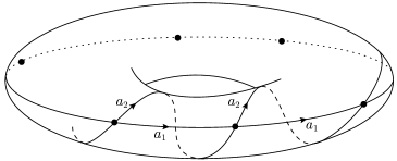
Figure 1. $T(a_{1},a_{2})$: the preimage in $\hat{K}$ of the torus in $K$ spanned by $a_{1}$ and $a_{2}$.

Note that this is exactly the mapping torus $\operatorname{Map}(B,\sigma)$ of $B=S^{1}$ (cellulated with $n$ vertices and $n$ edges labelled $a_{1}$) by the map $\sigma$ which is rotation by $2\pi/n$.

Let $\lambda$ be the loop in $B$ spelling out $a_{1}^{n}$; this is a generator for $\pi_{1}(B)$. Van Kampen’s theorem then gives us a presentation for the fundamental group of the mapping torus $\operatorname{Map}(B,\sigma)$, namely $\big{\langle}\lambda,t\;{\big{|}}\;[\lambda,t]\big{\rangle}$, where the stable letter $t$ represents the path $a_{1}a_{2}^{-1}$ in $T(a_{1},a_{2})$.

Now observe that $\hat{K}$ can be obtained (up to isometry—we are only changing the cell structure) from $\operatorname{Map}(B,\sigma)$ by again forming a mapping torus, this time by the shift map $\sigma^{\prime}$ that rotates each coordinate circle in $T(a_{1},a_{2})$ by $2\pi/n$. Again we can compute $\pi_{1}(\hat{K})$ using van Kampen’s theorem, and we find that

$$\pi_{1}(\hat{K})=\big{\langle}\lambda,t,t^{\prime}\;{\big{|}}\;[\lambda,t],[\lambda,t^{\prime}],[t,t^{\prime}]\big{\rangle},$$

where the new stable letter $t^{\prime}$ is the loop $a_{1}a_{3}^{-1}$. This presentation is efficient.

Remark 4.1.

To get an efficient presentation, we needed to work with a different $\operatorname{CAT}(0)$ cellulation to the obvious lifted cubical structure. In fact, the $2$-skeleton of a cube complex $L$ of dimension $\geq 3$ will almost never give an efficient presentation for its fundamental group: unless the boundary identifications turn it into a torus, any $3$-cube provides an obvious essential $2$-sphere in $L^{(2)}$ showing that one of the relations is redundant.

4.2. The main construction

We now turn to the general case when $\Sigma$ is an arbitrary connected finite flag complex. Let $N$ be the number of vertices in $\Sigma$, and fix an integer $n\geq 1$. We are going to construct an Eilenberg–Mac Lane space $Y^{n}_{N}$ for the group $\Gamma_{n}\subset G_{\Sigma}$ as an $N$-fold iterated mapping torus.

Order the vertices of $\Sigma$, $a_{1}<a_{2}<\cdots<a_{N}$, in such a way that $a_{j}$ is contained in the union of the closed stars of the $a_{i}$ with $i<j$. Let $Y^{n}_{1}$ be a circle, with cell structure consisting of $n$ vertices labelled $0,\ldots,n-1$, and $n$ edges, each labelled $a_{1}$. We write $\alpha_{1}$ for the generator $a_{1}^{n}$ of $\pi_{1}(Y^{n}_{1})$, and take $\mathscr{P}^{n}_{1}=\big{\langle}\alpha_{1}\;{\big{|}}\;\leavevmode\nobreak\ \big{\rangle}$ as a presentation for $\pi_{1}(Y^{n}_{1})$.

Suppose inductively that $Y^{n}_{k-1}$ has been defined and that for $1\leq i\leq k-1$, we have a circle $\alpha_{i}$ in $Y^{n}_{k-1}$ cellulated as the vertices $0,\ldots,n-1$ joined in cyclic order by edges labelled $a_{i}$. Let

$$S_{k}=\{v\;{\big{|}}\;v<v_{k}\text{ and }\{v,v_{k}\}\text{ is an edge in }\Sigma\}$$

and let $B\subset Y_{k-1}^{n}$ be the union of the loops $\alpha_{i}$ corresponding to vertices $v_{i}$ in $S_{k}$ (Figure 2), together with any higher-dimensional cells whose intersection with the $1$-skeleton of $Y_{k-1}^{n}$ is contained in this union.

Figure 2. The $1$-skeleton of the base space $B\subset Y^{n}_{k-1}$ for the next mapping torus in our inductive construction.

Lemma 4.2.

If $\Sigma$ is $1$-dimensional, then at the $k$th stage of this process the fundamental group of the base space $B$ is free of rank $1+n(\lvert S_{k}\rvert-1)$.

Proof.

If $\Sigma$ is $1$-dimensional then $B$ is a graph with $n$ vertices and $n\lvert S_{k}\rvert$ edges. ∎

There is an obvious label-preserving shift map $\sigma:B\to B$, which permutes the vertices of each $\alpha_{i}$ as the $n$-cycle $(0\leavevmode\nobreak\ 1\leavevmode\nobreak\ \cdots\leavevmode\nobreak\ n-1)$. We glue the mapping torus of $\sigma$ into $Y^{n}_{k-1}$ along $B$ to form $Y^{n}_{k}$. In the obvious cell structure on the mapping torus, there are new $1$-cells joining $p$ and $p+1$ (mod $n$) for $p=0,\ldots,n-1$: we label each of these by $a_{k}$. Then $\alpha_{k}=a_{k}^{n}$ is a loop in $Y_{k}^{n}$. By the Seifert–van Kampen theorem, we can obtain a presentation $\mathscr{P}^{n}_{k}$ for $\pi_{1}(Y_{k}^{n})$ by adding to $\mathscr{P}^{n}_{k-1}$ a single generator $t_{k}=a_{k}a_{j}^{-1}$ (where $a_{j}<a_{k}$ is a choice of vertex containing $a_{k}$ in its star), and for each element in a generating set for $\pi_{1}(B)$ a relation describing the action of $t_{k}$ on that generator.

Remark 4.3.

When $\Sigma$ is a graph, this construction of a presentation is really algorithmic: indeed, we shall write down the presentations it produces explicitly in $\S$ 5. The complication for higher-dimensional $\Sigma$ is that the base spaces of the mapping tori will be not be as simple as the ‘necklaces’ that occur in the $1$-dimensional case: in fact, their fundamental groups can be quite complicated, and finding a suitable generating set for these groups is already non-trivial. Although presentations of the form we have described still exist abstractly in this case, writing them down concretely is no longer straightforward (cf. $\S$ 6).

We are now in a position to prove Proposition A.

Proposition 4.4.

Let $\Sigma$ be a connected finite flag complex. For each integer $n\geq 1$, there is a generating set for $\Gamma_{n}=H_{\Sigma}\rtimes n\mathbf{Z}$ indexed by the vertices of $\Sigma$, and $\Gamma_{n}$ cannot be generated by fewer elements.

Proof.

The first assertion is immediate from the construction above. (Alternatively, one can observe that if $\Sigma^{(0)}=\{a_{1},\ldots,a_{N}\}$ then $H$ is generated by the elements $a_{1}a_{i}^{-1}$ with $i>1$ and $\Gamma_{n}$ is generated by these elements together with $a_{1}^{n}$.)

To see that $\Gamma_{n}$ cannot be generated by fewer than $N=\lvert\Sigma^{(0)}\rvert$ elements, one simply observes that $\dim_{\mathbf{Q}}H_{1}(G;\mathbf{Q})=N$ and $\Gamma_{n}$ has finite index in $G$, so $\dim_{\mathbf{Q}}H_{1}(\Gamma_{n};\mathbf{Q})\leq N$. ∎

4.3. Calculating the deficiency

For the remainder of this section we shall assume that $\Sigma$ is a finite flag graph; we retain the notation of the previous subsection.

Theorem 4.5.

The space $Y^{n}_{N}$ is non-positively curved and has fundamental group $\Gamma_{n}$. Moreover, $\mathscr{P}^{n}_{N}$ is a presentation of $\Gamma_{n}$ with $N$ generators and $N-1+n(1-\chi(\Sigma))$ relations, and this presentation is efficient.

Proof.

If we metrize each $\alpha_{i}$ as a circle of length $n$ then all our gluing maps are isometries, and it follows immediately from [4, II.11.13] that $Y^{n}_{N}$ is non-positively curved. The labels on the $1$-cells of $Y^{n}_{N}$ show how to define a covering projection from $Y^{n}_{N}$ to the standard $\mathrm{K}(G_{\Sigma},1)$; by construction, this cover is regular and $\Gamma_{n}$ is its fundamental group. Our presentation is obtained from a free group by repeated HNN extensions along free subgroups, so the corresponding one-vertex $2$-complex is aspherical [18, Proposition 3.6]; indeed, it is visibly homotopy equivalent to $Y^{n}_{N}$, which is aspherical since it is non-positively curved. Consequently the presentation is efficient. Finally, by Lemma 4.2 the number of relations is

$$\sum_{i=2}^{N}\big{(}1+n(\lvert S_{i}\rvert-1)\big{)}=N-1+n(1-\chi(\Sigma)).$$

∎

Remark 4.6.

The complex $Y^{n}_{N}$ is homeomorphic to the $n$-sheeted cover of the standard cubical $\mathrm{K}(G_{\Sigma},1)$ with fundamental group $\Gamma_{n}$, but we have given it a different cell structure.

Corollary 4.7.

When $\Sigma$ is a graph,

$$\operatorname{def}(\Gamma_{n})=1+n(\chi(\Sigma)-1).$$

In particular, $\operatorname{def}(\Gamma_{n})\to\infty$ as $n\to\infty$ if and only if $H_{\Sigma}$ fails to be finitely presented.

Proof.

Since $\mathscr{P}^{n}_{N}$ is efficient, it realizes the deficiency of the group. ∎

Remark 4.8.

The proof of Theorem 4.5 breaks down if $\Sigma$ has dimension $>1$: the question of when we obtain presentations realizing the deficiencies of the $\Gamma_{n}$ in this way is a delicate one.

5. Explicit presentations when $\Sigma$ is triangle-free

In $\S$ 4 we gave an algorithm that, in principle, one can apply to obtain efficient presentations for the groups $\Gamma_{n}$ associated to a finite $1$-dimensional flag complex $\Sigma$. The purpose of this section is to actually carry out this procedure and thus write down completely explicit presentations for the groups $\Gamma_{n}$.

5.1. A special case

Before presenting the general case, we first describe the particular case when $\Sigma$ is a cyclic graph of length $6$, with vertices ordered as shown in Figure 3.

Figure 3. The complex $\Sigma$ in $\S$ 5.1

There are two reasons for this: firstly, the notation in the general case is unwieldy, and it is helpful to first consider this simpler situation, which contains all the essential ideas; and secondly we shall later build on this example when we discuss $2$-dimensional flag complexes.

Let us fix $n$ and work through the construction of $\S$ 4.2 for the group $\Gamma_{n}$.

1. Our initial space $Y_{1}$ is the circle with its $n$-vertex cellulation. Each edge is labelled $a_{1}$, and the presentation we take for $\pi_{1}(Y_{1})$ is

   $$\mathscr{P}_{1}=\big{\langle}\lambda\;{\big{|}}\;\big{\rangle},$$

   where $\lambda$ is the loop $a_{1}^{n}$. From now on we shall abuse notation and write $\lambda=a_{1}^{n}$.

2. We form a mapping torus by the degree $1$ shift map, which rotates the base circle by $2\pi/n$; on the fundamental group, this has the effect of an HNN extension with stable letter $t_{2}=a_{2}a_{1}^{-1}$, and our second presentation is

   $$\mathscr{P}_{2}=\big{\langle}\lambda,t_{2}\;{\big{|}}\;[t_{2},\lambda]\big{\rangle}.$$

3. The base space is the circle $a_{2}^{n}=t_{2}^{n}\lambda$; our new stable letter is $t_{3}=a_{3}a_{2}^{-1}$, and our next presentation is

   $$\mathscr{P}_{3}=\big{\langle}\lambda,t_{2},t_{3}\;{\big{|}}\;[t_{2},\lambda],[t_{3},t_{2}^{n}\lambda]\big{\rangle}.$$

4. The base of our mapping torus is now the circle

   $$a_{3}^{n} =(a_{3}^{n}a_{2}^{-n})(a_{2}^{n}a_{1}^{-n})a_{1}^{n}$$

   $$=t_{3}^{n}t_{2}^{n}\lambda,$$

   and with respect to the stable letter $t_{4}=a_{4}a_{3}^{-1}$ our presentation is

   $$\mathscr{P}_{4}=\big{\langle}\lambda,t_{2},t_{3},t_{4}\;{\big{|}}\;[t_{2},\lambda],[t_{3},t_{2}^{n}\lambda],[t_{4},t_{3}^{n}t_{2}^{n}\lambda]\big{\rangle}.$$

   Notice that our relations include a path back to the initial vertex of $\Sigma$, which acts as a global basepoint.

5. In just the same way, we add another stable letter $t_{5}=a_{5}a_{4}^{-1}$ and get a presentation

   $$\mathscr{P}_{5}=\big{\langle}\lambda,t_{2},t_{3},t_{4},t_{5}\;{\big{|}}\;[t_{2},\lambda],[t_{3},t_{2}^{n}\lambda],[t_{4},t_{3}^{n}t_{2}^{n}\lambda],[t_{5},t_{4}^{n}t_{3}^{n}t_{2}^{n}\lambda]\big{\rangle}.$$

6. We now come to the final vertex, $a_{6}$. This has two predecessor vertices in our ordering, namely $a_{1}$ and $a_{5}$, so the base space $B$ for the final mapping torus is a necklace with two strands (cf. Figure 2): one has edges labelled $a_{1}$ and the other has edges labelled $a_{5}$. Let us choose and name a set of generators for $\pi_{1}(B)$, which is a free group of rank $n+1$:

   $$w_{0} =a_{5}a_{1}^{-1}=(a_{5}a_{4}^{-1})(a_{4}a_{3}^{-1})(a_{3}a_{2}^{-1})(a_{2}a_{1}^{-1})=t_{5}t_{4}t_{3}t_{2}$$

   $$w_{1} =a_{5}w_{0}a_{5}^{-1}=(a_{5}^{2}a_{4}^{-2})(a_{4}^{2}a_{3}^{-2})(a_{3}^{2}a_{2}^{-2})(a_{2}^{2}a_{1}^{-2})(a_{1}a_{5}^{-1})=t_{5}^{2}t_{4}^{2}t_{3}^{2}t_{2}^{2}w_{0}^{-1}$$

   $$w_{2} =a_{5}^{2}w_{0}a_{5}^{-2}=t_{5}^{3}t_{4}^{3}t_{3}^{3}t_{2}^{3}w_{0}^{-1}w_{1}^{-1}$$

   $$\ldots$$

   $$w_{n-1} =a_{5}^{n-1}w_{0}a_{5}^{1-n}=t_{5}^{n}t_{4}^{n}t_{3}^{n}t_{2}^{n}w_{0}^{-1}w_{1}^{-1}\cdots w_{n-2}^{-1}$$

   $$\alpha_{5} =a_{5}^{n}=t_{5}^{n}t_{4}^{n}t_{3}^{n}t_{2}^{n}\lambda.$$

   If we take our stable letter to be $t_{6}=a_{6}a_{5}^{-1}$ then we can work out how $t_{6}$ acts on these generators:

   $$t_{6}w_{0}t_{6}^{-1} =a_{5}^{-1}w_{0}a_{5}=a_{5}^{-n}a_{5}^{n-1}w_{0}a_{5}^{1-n}a_{5}^{n}=\alpha_{5}^{-1}w_{n-1}\alpha_{5}$$

   $$t_{6}w_{1}t_{6}^{-1} =a_{5}^{-1}a_{5}w_{0}a_{5}^{-1}a_{5}=w_{0}$$

   $$\ldots$$

   $$t_{6}w_{n-1}t_{6}^{-1} =w_{n-2}$$

   $$t_{6}\alpha_{5}t_{6}^{-1} =\alpha_{5}.$$

   Therefore our final presentation for $\Gamma_{n}$ is

   $$\mathscr{P}_{6}=\big{\langle}\lambda,t_{2},t_{3},t_{4},t_{5},t_{6}\;{\big{|}}\;[t_{2},\lambda],[t_{3},t_{2}^{n}\lambda],[t_{4},t_{3}^{n}t_{2}^{n}\lambda],[t_{5},t_{4}^{n}t_{3}^{n}t_{2}^{n}\lambda],\\ [t_{6},t_{5}^{n}t_{4}^{n}t_{3}^{n}t_{2}^{n}\lambda],\mathscr{F}_{n}\big{\rangle},$$

   where

   $$\mathscr{F}_{n}=\begin{cases}t_{6}w_{0}t_{6}^{-1}=\alpha_{5}^{-1}w_{n-1}\alpha_{5}\\ t_{6}w_{i}t_{6}^{-1}=w_{i-1}&(i=1,\ldots,n-1).\end{cases}$$

5.2. The general case

Now let $\Sigma$ be any finite $1$-dimensional flag complex. Choose a maximal tree $T\subset\Sigma$, and as in $\S$ 4.2 fix an ordering $v_{1}<\cdots<v_{N}$ of the vertices of $\Sigma$ such that each vertex (apart from $v_{1}$) is adjacent to some vertex that precedes it. Given a pair of vertices $v$ and $v^{\prime}$ in $\Sigma$, there is a unique path $(v=v_{p_{1}},v_{p_{2}},\ldots,v_{p_{s}}=v^{\prime})$ from $v$ to $v^{\prime}$ in $T$. Set

$$\theta^{i}(v,v^{\prime})=t_{p_{1}}^{i}t_{p_{2}}^{i}\cdots t_{p_{k-1}}^{i}.$$

(For the moment, these are just formal words in the alphabet $\{t_{i}\}$.)

As always, we start with the presentation $\mathscr{P}_{1}=\big{\langle}\lambda\;{\big{|}}\;\big{\rangle}$. Suppose inductively that we have constructed the presentation $\mathscr{P}_{k-1}$. There is a distinguished predecessor of $v_{k}$ in our order, namely the unique vertex $v_{\alpha}<v_{k}$ such that $v_{\alpha}$ and $v_{k}$ are connected by an edge in the maximal tree $T$. There might also be other vertices $v_{\beta_{1}},\ldots,v_{\beta_{r}}$ such that $v_{\beta_{i}}<v_{k}$ and $v_{\beta_{i}}$ is adjacent to $v_{k}$ in $\Sigma$ (so here $r\geq 0$). The base space $B$ for the next mapping torus in our construction is now a necklace with $r+1$ strands, and choosing a presentation for $\pi_{1}(B)$ amounts to choosing a maximal tree in $B$. We take this tree to be $a_{\alpha}^{n-1}$, where $v_{\alpha}$ is our distinguished vertex. For the purposes of our presentation, the stable letter for the next HNN extension will be $t_{k}=a_{k}a_{\alpha}^{-1}$.

This gives us the following generating set for $\pi_{1}(B)$:

$$\left.\begin{aligned} w_{i,0}&=\theta^{1}(v_{k},v_{\beta_{i}})\\ w_{i,1}&=\theta^{2}(v_{k},v_{\beta_{i}})w_{i,0}^{-1}\\ w_{i,2}&=\theta^{3}(v_{k},v_{\beta_{i}})w_{i,0}^{-1}w_{i,1}^{-1}\\ &\;\;\ldots\\ w_{i,n-1}&=\theta^{n}(v_{k},v_{\beta_{i}})w_{i,0}^{-1}w_{i,1}^{-1}\cdots w_{i,n-2}^{-1}\\ \end{aligned}\quad\right\}\qquad i=1,\ldots r,$$

together with $\gamma_{k}=a_{\alpha}^{n}=\theta^{n}(v_{\alpha},v_{1})\lambda$; the stable letter acts by

$$t_{k}w_{i,0}t_{k}^{-1} =\gamma_{k}^{-1}w_{i,n-1}\gamma_{k}$$

$$t_{k}w_{i,j}t_{k}^{-1} =w_{i,j-1}\quad(j=1,\ldots,n-1)$$

$$[t_{k},\gamma_{k}] =1.$$

Let $\mathscr{F}_{n,k}$ be the family of relations describing this action of the stable letter on all the words $w_{i,j}$ for $1\leq i\leq r$ and $0\leq j\leq n-1$, a total of $rn$ relations. (If $v_{k}$ is not adjacent to any of its predecessors by an edge not in the tree $T$, then $\mathscr{F}_{n,k}$ is empty.) We set

$$\mathscr{P}_{k}=\mathscr{P}_{k-1}\cup\big{\langle}t_{k}\;{\big{|}}\;[t_{k},\gamma_{k}],\mathscr{F}_{n,k}\big{\rangle}.$$

Theorem 5.1.

The presentation $\mathscr{P}_{N}$ is an efficient presentation of $\Gamma_{n}$.

Proof.

This is immediate from the construction and Theorem 4.5. ∎

Remark 5.2.

The choice of a maximal tree in $\Sigma$ is the key technical ingredient needed to pass from the special case of $\S$ 5.1 to the general case: it provides a consistent way to choose bases for the fundamental groups of the successive base spaces for the mapping tori.

6. Extension to $2$-complexes: theoretical limitations

6.1. The initial aim

In $\S$ 4 we described an algorithm to write down explicit presentations of the groups $\Gamma_{n}\subset G_{\Sigma}$ associated to a $1$-dimensional flag complex $\Sigma$ on a generating set of size $N=\lvert\Sigma^{(0)}\rvert$ and with $R(n,\Sigma)$ relations, where $\lim_{n\to\infty}R(n,\Sigma)<\infty$ if and only if the Bestvina–Brady kernel $H_{\Sigma}$ is finitely presented. One naturally seeks to generalize this to arbitrary finite flag complexes $\Sigma$ and again construct efficient presentations of $\Gamma_{n}$ explicitly; in particular we should like to be able to prove the following conjecture:

Conjecture 6.1.

If $\Sigma$ is not simply connected, then $\operatorname{def}(\Gamma_{n})\to\infty$ as $n\to\infty$.

The purpose of this section is to show that there is a logical obstruction to establishing this conjecture simply by constructing explicit presentations realizing the deficiencies of the $\Gamma_{n}$.

6.2. A computability obstruction

Theorem 6.2.

Suppose there is an algorithm that generates a finite presentation $\big{\langle}A(\Sigma)\;{\big{|}}\;R(n,\Sigma)\big{\rangle}$ of $\Gamma_{n}$ for each pair $(n,\Sigma)$ with $n$ a positive integer and $\Sigma$ a finite flag complex. Suppose further that there is a partial algorithm that will correctly determine that $\sup_{n}\lvert R(n,\Sigma)=\infty\rvert$ if $\Sigma$ belongs to a certain collection $\mathscr{C}$ of finite flag complexes. Then $\mathscr{C}$ does not coincide with the complement of the class of simply connected finite flag complexes.

Proof.

Suppose that $\mathscr{C}$ is indeed the class of non-simply-connected finite flag complexes. Then there is a partial algorithm that takes a finite presentation and recognizes that that group it presents is non-trivial: form the presentation $2$-complex, barycentrically subdivide until one has a flag complex, then apply the partial algorithm hypothesized in the statement of the theorem. But it is well known that no such partial algorithm exists (see, for example, [17, Corollary 12.33]). ∎

6.3. A revised aim

Although Theorem 6.2 rules out the possibility of a constructive proof of Conjecture 6.1 in general, we can nonetheless seek a widely-applicable and effective procedure that will produce small presentations of $\Gamma_{n}$ for a large class $\mathscr{C}$ of $2$-complexes. In particular, if $\mathscr{C}$ is a class in which triviality of $\pi_{1}$ can be algorithmically determined, then we might still hope for a complete algorithm: for example, if $\mathscr{C}$ is the class of flag triangulations of compact surfaces, or the class of negatively-curved $2$-complexes. We discuss the first of these classes in $\S$ 8.2.

7. Extension to $2$-complexes: simplifying presentations

In this section we give examples where one can see explicitly how simplifying the topology of $\Sigma$ (for example, by adding a $2$-simplex to kill its boundary loop in $\pi_{1}$) translates into a simplification of the presentations of the corresponding groups $\Gamma_{n}\subset G_{\Sigma}$.

7.1. Mapping torus constructions for $2$-complexes

Rather than applying the construction of $\S$ 4.2 directly to an arbitrary flag complex, we try to simplify the combinatorics in such a way that we can build directly on what we have done in the $1$-dimensional case. Throughout this section, we assume that $\Sigma$ has been obtained by barycentrically subdividing another complex $\Delta$. (Of course, this has no significance from the point of view of topology.) Let $\Sigma_{1}$ be the subcomplex of the $1$-skeleton of $\Sigma$ obtained by deleting the vertices at the barycentres of the $2$-simplices of $\Delta$, together with the edges emanating from these vertices.

We begin by choosing a maximal tree $T$ in $\Sigma_{1}$ and building a presentation for $\Gamma_{n}\subset G_{\Sigma_{1}}$, exactly as in $\S$ 4.2. This will have a collection of size $n$ families of relations, indexed by the edges in the complement of $T$ in $\Sigma_{1}$.

We now consider adding in the missing vertices, ‘building over’ the $2$-simplices of $\Delta$. Each $2$-simplex $\sigma$ contributes a $3$-torus to the standard Eilenberg–Mac Lane space for our groups, which is exactly the mapping torus of the degree $1$ shift map on the union of $2$-tori corresponding to the edges in the boundary of $\sigma$. In terms of $\pi_{1}$, we add a new stable letter $\tau_{\sigma}$ and six relations describing its action on a generating set for the fundamental group of the base of the mapping torus. In the edge-path groupoid, $\tau_{\sigma}$ is equal to $b_{\sigma}a_{i}^{-1}$ for some $i$, where $b_{\sigma}^{n}$ is the path traversing once the copy of $S^{1}$ corresponding to the vertex at the centre of $\sigma$, and $a_{i}$ is one of the vertices in the boundary of $\sigma$. Another way of thinking about this is that we are extending our maximal tree from $\Sigma_{1}$ to a maximal tree for the whole $1$-skeleton of $\Sigma$, adjoining the edges $(b_{\sigma},a_{i})$.

We are going to examine how these extra relations can be used to eliminate size $n$ families of relations picked up in the first part of the construction, which only involved $\Sigma_{1}$.

7.2. A local argument: completing a 2-simplex

We start by discussing in detail the simplest case, namely when $\Sigma$ is a $2$-simplex, barycentrically subdivided. Then $\Sigma_{1}$ is exactly the flag graph we analysed in $\S$ 5.1, so we will adopt the same notation as there: order the vertices in the boundary of the simplex as in Figure 3, with the $i$th vertex called $a_{i}$, and let $Y_{6}$ be the $2$-complex we finished up with at the end of $\S$ 5.1. We shall call the extra vertex at the barycentre of the $2$-simplex $b$; it will come after all the $a_{i}$ in our order.

We can make a $3$-complex isometric to the cover of the standard Eilenberg–Mac Lane space corresponding to the index $n$ subgroup $\Gamma_{n}\subset G_{\Sigma}$ by forming the mapping torus of $Y_{6}$ by the map $\sigma$ that acts as a degree $1$ shift on each circle $a_{i}^{n}$ in $Y_{6}$.

The base $Y_{6}$ is a union of six tori, glued along coordinate circles. Its fundamental group is generated by $\lambda,t_{2},\ldots,t_{6}$, and we can get a presentation for the fundamental group $\Gamma_{n}$ of the mapping torus of $\sigma$ by saying how a stable letter $\tau=ba_{5}^{-1}$ acts on these generators. For example, one calculates that

$$\tau t_{4}\tau^{-1} =ba_{5}^{-1}a_{4}a_{3}^{-1}a_{5}b^{-1}$$

$$=a_{4}a_{5}^{-1}a_{3}^{-1}a_{5}$$

$$=t_{5}^{-1}(a_{3}^{-1}a_{4})(a_{4}^{-1}a_{5})$$

$$=t_{5}^{-1}t_{4}t_{5},$$

and similarly for the other generators. The resulting presentation is

$$\Gamma_{n}=\big{\langle}\lambda,t_{2},t_{3},t_{4},t_{5},t_{6},\tau\;{\big{|}}\;[t_{2},\lambda],[t_{3},t_{2}^{n}\lambda],[t_{4},t_{3}^{n}t_{2}^{n}\lambda],[t_{5},t_{4}^{n}t_{3}^{n}t_{2}^{n}\lambda],\\ [t_{6},t_{5}^{n}t_{4}^{n}t_{3}^{n}t_{2}^{n}\lambda],\mathscr{F}_{n},\mathscr{G}\big{\rangle},$$

where $\mathscr{F}_{n}$ is as in $\S$ 5.1 and

$$\mathscr{G}=\begin{cases}[\tau,t_{6}],\\ [\tau,t_{5}],\\ \tau t_{4}\tau^{-1}=t_{5}^{-1}t_{4}t_{5},\\ \tau t_{3}\tau^{-1}=t_{5}^{-1}t_{4}^{-1}t_{3}t_{4}t_{5},\\ \tau t_{2}\tau^{-1}=t_{5}^{-1}t_{4}^{-1}t_{3}^{-1}t_{2}t_{3}t_{4}t_{5},\\ \tau\lambda\tau^{-1}=t_{6}\lambda t_{6}^{-1}.\end{cases}$$

We know from Theorem F that the groups $\Gamma_{n}$ have presentations in which the number of relations does not go to infinity with $n$, so for large $n$ this presentation will have many superfluous relations. Our aim is to see how one can eliminate the size $n$ family $\mathscr{F}_{n}$. Specifically, we will prove:

Proposition 7.1.

$\Gamma_{n}$ admits the following presentation:

$$\Gamma_{n}=\big{\langle}\lambda,t_{2},t_{3},t_{4},t_{5},t_{6},\tau\;{\big{|}}\;[t_{2},\lambda],[t_{3},t_{2}^{n}\lambda],[t_{4},t_{3}^{n}t_{2}^{n}\lambda],[t_{5},t_{4}^{n}t_{3}^{n}t_{2}^{n}\lambda],\\ [t_{6},t_{5}^{n}t_{4}^{n}t_{3}^{n}t_{2}^{n}\lambda],\mathscr{G},[t_{6}^{-1}\tau,w_{0}]\big{\rangle}.$$

Corollary 7.2.

$\operatorname{def}(\Gamma_{n})\leq 5$.

The proposition is a consequence of the following three lemmas.

Lemma 7.3.

The relation

($$* [t_{6}^{-1}\tau,w_{0}]=1$$)

holds in $\Gamma_{n}$.

Proof.

One has

$$t_{6}^{-1}\tau w_{0}\tau^{-1}t_{6} =t_{6}^{-1}(t_{5}^{\tau})(t_{4}^{\tau})(t_{3}^{\tau})(t_{2}^{\tau})t_{6}$$

$$=t_{6}^{-1}t_{5}t_{5}^{-1}t_{4}t_{5}t_{5}^{-1}t_{4}^{-1}t_{3}t_{4}t_{5}t_{5}^{-1}t_{4}^{-1}t_{3}^{-1}t_{2}t_{3}t_{4}t_{5}t_{6}$$

$$=t_{6}^{-1}t_{2}t_{3}t_{4}t_{5}t_{6}$$

$$=a_{5}a_{1}^{-1}$$

$$=w_{0}.$$

∎

Remark 7.4.

We are using here the geometric interpretation of $\Gamma_{n}$ as $\pi_{1}(Y_{6})$, and working in the edge-path groupoid of $Y_{6}$. We need to do this (and pick up the relation in the lemma) because the raw presentation does not tell us how $t_{6}$ acts on the lower $t_{i}$, although we know how $\tau$ acts on them. This is, in a sense, the key point: $t_{6}$ acts on $T(a_{1},a_{5})$, whereas $\tau$ acts on the whole base $B$. Before, we had to spell out how $t_{6}$ acts on all the $w_{i}=w_{i}(\lambda,t_{2},\ldots,t_{5})$, but now we can make do with a single relation saying that its action is the same as the action of $\tau$: we know how $\tau$ acts on the $w_{i}$ because we know how it acts on all the $t_{i}$.

Lemma 7.5.

Let $\mathscr{F}_{n}^{\prime}$ be the family obtained from $\mathscr{F}_{n}$ by replacing all occurrences of $t_{6}$ with $\tau$. The relations $\mathscr{F}_{n}^{\prime}$ follow from $\mathscr{G}$.

Proof.

This is a routine inductive calculation. For example,

$$\tau w_{1}\tau^{-1} =\tau t_{5}^{2}t_{4}^{2}t_{3}^{2}t_{2}t_{3}^{-1}t_{4}^{-1}t_{5}^{-1}\tau^{-1}$$

$$=t_{5}^{2}t_{5}^{-1}t_{4}^{2}t_{5}t_{5}^{-1}t_{4}^{-1}t_{3}^{2}t_{4}t_{5}t_{5}^{-1}t_{4}^{-1}t_{3}^{-1}t_{2}^{2}t_{3}t_{4}t_{5}t_{5}^{-1}t_{4}^{-1}t_{3}^{-1}t_{2}^{-1}t_{3}t_{4}t_{5}$$

$$\hphantom{==}t_{5}^{-1}t_{4}^{-1}t_{3}^{-1}t_{4}t_{5}t_{5}^{-1}t_{4}^{-1}t_{5}t_{5}^{-1}\quad\text{ (making }\tau\text{ act throughout)}$$

$$=t_{5}t_{4}t_{3}t_{2}$$

$$=w_{0}.$$

∎

Lemma 7.6.

The relations $\mathscr{F}_{n}$ follow from $\mathscr{F}_{n}^{\prime}$, the relation $(*)$, and $[t_{6},\alpha_{5}]$.

Proof.

Again, this is no more than a simple combinatorial calculation. That $t_{6}$ acts as desired on $w_{0}$ is immediate from $(*)$, and one can then prove the same for $w_{n-k}$ by induction on $k$: thus,

$$t_{6}w_{n-1}t_{6}^{-1} =t_{6}\alpha_{5}\tau w_{0}\tau^{-1}\alpha_{5}^{-1}t_{6}^{-1} \text{using }\mathscr{F}_{n}^{\prime}$$

$$=\tau\alpha_{5}t_{6}w_{0}t_{6}^{-1}\alpha_{5}^{-1}\tau^{-1} \text{since }t_{6}\text{ commutes with }\alpha_{5}\text{ and }\tau$$

$$=\tau w_{n-1}\tau^{-1}$$ by the inductive hypothesis

$$=w_{n-2} \text{using }\mathscr{F}_{n}^{\prime}\text{ again}$$

and similarly for $w_{n-2},\ldots,w_{1}$, except that $\alpha_{5}$ no longer appears. ∎

7.3. A local argument: completing a $2$-simplex with two ‘missing edges’

We now show how two of our size $n$ families of relations can be consolidated into a single family in the presence of a $2$-simplex.

Let us consider, then, the complex $\Sigma$ shown in Figure 4.

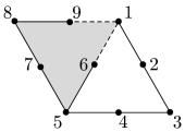
Figure 4. The complex $\Sigma$ in $\S$ 7.3. We will fill in the left triangle with a (subdivided) $2$-simplex.

We order the vertices as indicated in the figure. Following through our procedure once again, we obtain a presentation $\mathscr{P}_{9}$ for $Y_{9}$. We are going to modify this presentation slightly by performing a Tietze move: we shall introduce a new generator $\theta$, which we set equal to the word $t_{6}t_{5}t_{4}t_{3}t_{2}$ in the other generators. (In the edge-path groupoid, $\theta$ is equal to $a_{6}a_{1}^{-1}$.) The resulting presentation is

$$\mathscr{P}=\big{\langle}\lambda,t_{2} ,t_{3},t_{4},t_{5},t_{6},t_{7},t_{8},t_{9},\theta\;{\big{|}}\;\theta=t_{6}t_{5}t_{4}t_{3}t_{2},$$

$$[t_{2},\lambda],[t_{3},t_{2}^{n}\lambda],[t_{4},t_{3}^{n}t_{2}^{n}\lambda],[t_{5},t_{4}^{n}t_{3}^{n}t_{2}^{n}\lambda],[t_{6},t_{5}^{n}t_{4}^{n}t_{3}^{n}t_{2}^{n}\lambda],\mathscr{F}_{n},$$

$$[t_{7},t_{5}^{n}t_{4}^{n}t_{3}^{n}t_{2}^{n}],[t_{8},t_{7}^{n}t_{5}^{n}t_{4}^{n}t_{3}^{n}t_{2}^{n}\lambda],[t_{9},t_{8}^{n}t_{7}^{n}t_{5}^{n}t_{4}^{n}t_{3}^{n}t_{2}^{n}\lambda],\mathscr{H}_{n}\big{\rangle},$$

where if

$$w_{0} =t_{5}t_{4}t_{3}t_{2}$$

$$w_{1} =t_{5}^{2}t_{4}^{2}t_{3}^{2}t_{2}^{2}w_{0}^{-1}$$

$$w_{2} =t_{5}^{3}t_{4}^{3}t_{3}^{3}t_{2}^{3}w_{0}^{-1}w_{1}^{-1}$$

$$\;\;\vdots$$

$$w_{n-1} =t_{5}^{n}t_{4}^{n}t_{3}^{n}t_{2}^{n}w_{0}^{-1}w_{1}^{-1}\cdots w_{n-2}^{-1}$$

$$\alpha =t_{5}^{n}t_{4}^{n}t_{3}^{n}t_{2}^{n}\lambda$$

and

$$u_{0} =t_{8}t_{7}t_{5}t_{4}t_{3}t_{2}$$

$$u_{1} =t_{8}^{2}t_{7}^{2}t_{5}^{2}t_{4}^{2}t_{3}^{2}t_{2}^{2}u_{0}^{-1}$$

$$\;\;\vdots$$

$$u_{n-1} =t_{8}^{n}t_{7}^{n}t_{5}^{n}t_{4}^{n}t_{3}^{n}t_{2}^{n}u_{0}^{-1}u_{1}^{-1}\cdots u_{n-2}^{-1}$$

$$\beta =t_{8}^{n}t_{7}^{n}t_{5}^{n}t_{4}^{n}t_{3}^{n}t_{2}^{n}\lambda$$

then

$$\mathscr{F}_{n}=\begin{cases}t_{6}w_{0}t_{6}^{-1}=\alpha^{-1}w_{n-1}\alpha\\ t_{6}w_{i}t_{6}^{-1}=w_{i-1}&(i=1,\ldots,n-1).\end{cases}$$

and

$$\mathscr{H}_{n}=\begin{cases}t_{9}u_{0}t_{9}^{-1}=\beta^{-1}u_{n-1}\beta\\ t_{9}u_{i}t_{9}^{-1}=u_{i-1}&(i=1,\ldots,n-1).\end{cases}$$

(cf. $\S$ 7.2).

We now complete $\Sigma$ by filling in the left-hand triangle with a (subdivided) $2$-simplex. As before, we obtain a $3$-dimensional $\mathrm{K}(\Gamma_{n},1)$ by forming the mapping torus of $Y_{9}$ by the degree-$1$ shift map on the $a_{i}^{n}$ for $i=1,5,6,7,8,9$. A set of $\pi_{1}$ generators for the base of this mapping torus is given by

$$a_{9}a_{8}^{-1} =t_{9}$$

$$a_{8}a_{7}^{-1} =t_{8}$$

$$a_{7}a_{5}^{-1} =t_{7}$$

$$a_{6}a_{5}^{-1} =t_{6}$$

$$a_{6}a_{1}^{-1} =\theta$$

$$a_{1}^{n} =\lambda,$$

and by the Seifert–van Kampen theorem we obtain a presentation for $\Gamma_{n}$ by adding to our presentation a stable letter $\tau$, and a collection of relations describing the action of $\tau$ on these generators. One checks easily that these relations are

$$\mathscr{G}=\begin{cases}[\tau,t_{9}],\\ [\tau,t_{8}],\\ \tau t_{7}\tau^{-1}=t_{8}^{-1}t_{7}t_{8},\\ \tau t_{6}\tau^{-1}=t_{8}^{-1}t_{7}^{-1}t_{6}t_{7}t_{8},\\ \tau\theta\tau^{-1}=t_{8}^{-1}t_{7}^{-1}t_{6}\theta t_{6}^{-1}t_{7}t_{8},\\ \tau\lambda\tau^{-1}=t_{8}^{-1}t_{7}^{-1}t_{6}\lambda t_{6}^{-1}t_{7}t_{8}.\end{cases}$$

Lemma 7.7.

The relation

($$* [t_{9}^{-1}\tau,u_{0}]=1$$)

holds in $\Gamma_{n}$.

Proof.

The proof is entirely analogous to that of Lemma 7.3. ∎

Lemma 7.8.

Let $\mathscr{H}^{\prime}_{n}$ be the family of words obtained from $\mathscr{H}_{n}$ be replacing all occurrences of $t_{9}$ with $\tau$. The relations $\mathscr{H}^{\prime}_{n}$ follow from $\mathscr{F}_{n}$ and $\mathscr{G}$.

Proof.

This is another straightforward induction: we present a sample calculation. Observe that $u_{1}=t_{8}^{2}t_{7}^{2}w_{1}t_{7}^{-1}t_{8}^{-1}$, and $w_{1}=t_{6}^{-1}w_{0}t_{6}=t_{6}^{-2}\theta t_{6}$. Thus

$$\tau u_{1}\tau^{-1} =(t_{8}^{\tau})^{2}(t_{7}^{\tau})^{2}(t_{6}^{\tau})^{-2}\theta^{\tau}t_{6}^{\tau}(t_{7}^{\tau})^{-1}(t_{8}^{\tau})^{-1}$$

$$=t_{8}^{2}t_{8}^{-1}t_{7}^{2}t_{8}t_{8}^{-1}t_{7}^{-1}t_{6}^{-2}t_{7}t_{8}t_{8}^{-1}t_{7}^{-1}t_{6}\theta t_{6}^{-1}t_{7}t_{8}t_{8}^{-1}t_{7}^{-1}t_{6}t_{7}t_{8}t_{8}^{-1}t_{7}^{-1}t_{8}^{-1}$$

$$=t_{8}t_{7}t_{6}^{-1}\theta$$

$$=u_{0}.$$

∎

Proposition 7.9.

The presentation obtained from $\mathscr{P}$ by replacing $\mathscr{H}_{n}$ by the relation $(*)$ is again a presentation of $\Gamma_{n}$.

Proof.

Given the previous two lemmas, it suffices to show that the relations $\mathscr{H}_{n}$ follow from $\mathscr{H}^{\prime}_{n}$, the relation $(*)$, and the other relations in $\mathscr{P}$. Just as in Lemma 7.6, this can be proved by a straightforward induction. ∎

7.4. A scheme for simplifying presentations for a general $2$-complex

Now consider a general $\Sigma$, obtained as before by barycentrically subdividing another complex $\Delta$. Recall that we have a presentation of $\Gamma_{n}\subset G_{\Sigma}$ with a size $n$ family of relations for each edge in the complement of a maximal tree $T$ in $\Sigma_{1}\subset\Sigma$, and for each $2$-simplex $\sigma$ in $\Delta$ we have a stable letter $\tau_{\sigma}$ and six relations describing its action on a generating set for the fundamental group of the base of the corresponding mapping torus.

The local arguments of $\S$ 7.2 and $\S$ 7.3 yield the following procedure.

Proposition 7.10.

One can eliminate (by which we mean replace by a single relation of the form $[\tau_{\sigma}t_{i},w_{0}]=1$) the family of relations corresponding to an edge $e$ in $\Sigma_{1}-T$ if $\Delta$ contains a $2$-simplex the boundary of whose image in $\Sigma$ is contained in $T\cup e$, or in $T\cup e\cup f$ (in this case, we keep the family of relations corresponding to $f\subset\Sigma_{1}-T$).

By repeated application of this proposition, we can potentially remove a family of relations from our presentation for each $2$-simplex of $\Delta$; thus by the end, we have $\geq 1-\chi(\Delta)$ families. In particular, if $\chi(\Delta)<1$ then we obtain a presentation for $\Gamma_{n}$ with $O(n)$ relations, as we expect. The interesting case is when $\chi(\Delta)=1$: in this case it is possible that we may be able to remove all of the size $n$ families. One might hope that this happens if and only if $H_{\Delta}$ is finitely presented, but we know from Theorem 6.2 that we cannot hope to create an algorithm exhibiting this, even if is true.

7.5. Presentations of the Bestvina–Brady kernels

An entirely analogous procedure to the one described above lets one obtain presentations for the Bestvina–Brady kernels themselves. In fact, we can derive these presentations purely formally from the ones we have found for $\Gamma_{n}$ by setting $n=\infty$ and discarding the generator $\lambda$.

It is interesting to compare the resulting presentations with those found by W. Dicks and I. Leary:

Theorem 7.11 ([9]).

If $\Sigma$ is connected, then the group $H_{\Sigma}$ has a presentation with generating set the directed edges of $\Sigma$, and relators all words of the form $e_{1}^{n}e_{2}^{n}\cdots e_{k}^{n}$ for $(e_{1},\ldots,e_{k})$ a directed cycle in $\Sigma$.

Our presentations are instead on a generating set indexed by the vertices of $\Sigma$, though in fact these generators are better thought of as directed edges: the generator associated to a vertex $v$ really corresponds to the edge in our chosen maximal tree from $v$ to its immediate predecessor. As $n\to\infty$, our families become infinite families, whose elements contain the characteristic subwords $t_{i_{1}}^{n}\cdots t_{i_{k}}^{n}$ for all integers $n$, where $(t_{i_{1}},\ldots,t_{i_{k}})$ is a path in the $1$-skeleton of $\Sigma$.

Both presentations of the kernel bring their own insights: in the Dicks–Leary presentation, one can see very clearly how non-trivial loops in $\pi_{1}(\Sigma)$ lead to infinite families of relations in the kernel, whereas our presentation has the benefit of being on a minimal generating set.

8. Extension to $2$-complexes: applications

8.1. Coning off an edge loop

For our first application, we show how killing a loop in $\pi_{1}(\Sigma)$ can allow us to remove a family of relations.

Proposition 8.1.

Let $\hat{\Sigma}$ be a complex obtained from $\Sigma$ by coning off an edge-loop $\ell$ in $\Sigma_{1}$, and let $\hat{\Gamma}_{n}=H_{\hat{\Sigma}}\rtimes n\mathbf{Z}$. Let $e\subset\Sigma_{1}$ be an edge in $\ell$ that does not lie in the maximal tree $T$. From the presentations of $\Gamma_{n}$ described in $\S$ 7.1, one can obtain presentations of $\hat{\Gamma}_{n}$ such that for each $n$, the family of relations corresponding to $e$ is removed and a fixed number of relations independent of $n$ is added.

Proof.

Extend the maximal tree in $\Sigma_{1}$ to a maximal tree $\hat{T}$ in $\hat{\Sigma}_{1}$ in such a way that it contains both ‘halves’ of the subdivided edge $\alpha$ from the cone point to $\partial e$ (Figure 5).

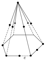
Figure 5. Coning off a loop in $\Sigma_{1}$.

We now start filling in $2$-simplices around the cone, starting with the one containing $\alpha$ but not $e$ in its boundary (for example, in Figure 5, this is the front-right simplex). In each case, we are able, using Proposition 7.10, to remove the family attached to the ‘missing’ edge between the cone point and $\Sigma_{1}$. When we come around to the last $2$-simplex, we have already eliminated this ‘vertical’ family, so we can instead use the $2$-simplex to eliminate the family corresponding to the edge $e$, again by Proposition 7.10. ∎

Remark 8.2.

One can view our argument that adding a subdivided $2$-simplex lets us remove one of the families on the boundary of that $2$-simplex as a special case of Proposition 8.1: the subdivided $2$-simplex is exactly the cone on its boundary.

Remark 8.3.

This argument shows that the number of size $n$ families of relations that we are left with in our presentation is bounded below by the killing number of $\pi_{1}(\Sigma)$: recall that a group $\Gamma$ has killing number $\leq k$ if $\Gamma$ is the normal closure of $k$ elements. In [14], J. Lennox and J. Wiegold prove that any finite perfect group has killing number $1$, and conjecture that the same is true for any finitely generated perfect group.

8.2. When $\Sigma$ is a triangulated surface

This simple situation illustrates clearly how a homotopically non-trivial loop can prevent one from removing all the families of relations.

Proposition 8.4.

Let $\Sigma$ be a standard flag triangulation of a compact surface and let $\Gamma_{n}$ be the corresponding Artin subgroups. Then repeated use of Proposition 7.10 produces a presentation of $\Gamma_{n}$ with $O(1)$ relations if and only if $\Sigma$ is homeomorphic to the disc or the sphere, i.e. if and only if $\Sigma$ is simply connected.

Remark 8.5.

It is interesting to compare this to the subdivided $2$-simplex we analysed in $\S$ 7.2: in each case, the Euler characteristic of the complex is $1$, but whereas in the former example our procedure allowed us to remove the single size $n$ family of relations in our presentation, in this case the topology prevents us from doing this. This underscores the fact that the presentation invariants we are examining are more subtle than just Euler characteristic, which in turn encourages the belief that the asymptotic behaviour of $\operatorname{def}(\Gamma_{n})$ should not depend only on the homology of $\Sigma$.

Proof of Proposition 8.4.

For surfaces of Euler characteristic $\leq 0$, our procedure gives us no hope of removing all of the infinite families. On the other hand, we have already seen in $\S$ 7.2 that the groups $\Gamma_{n}$ associated to the triangulation of the disc as a single $2$-simplex can be presented with $O(1)$ relations, while in any standard triangulation of the sphere the equator is coned off (cf. Proposition 8.1). Thus it only remains to consider the projective plane.

The ‘standard’ flag triangulation $\Sigma$ of $\mathbf{R}P^{2}$ is obtained from the complex $\Sigma_{1}$ shown in Figure 6 by filling in (subdivisions of) all the visible triangles.

Figure 6. $\Sigma_{1}$ when $\Delta$ is a triangulation of $\mathbf{R}P^{2}$.

We order the vertices as shown; we choose the maximal tree whose complement is the dotted lines. One checks that $\Sigma_{1}$ has $21$ vertices and $30$ edges, so $\operatorname{rk}(\pi_{1}(\Sigma_{1}))=10$, and thus in our presentation for $\Gamma_{n}$ we have $10$ size $n$ families of relations. Let us write $\mathscr{F}(a,b)$ for the family corresponding to the edge joining the vertices labelled $a$ and $b$.

To form $\Sigma$, we must now adjoin $10$ $2$-simplices; we shall refer to them by boldface numbers, as in Figure 6. Now we start to apply the simplification procedure described in Proposition 7.10:

$$\mathbf{4} \Rightarrow\mathscr{F}(1,6)$$

$$\mathbf{9} \Rightarrow\mathscr{F}(5,19)$$

$$\mathbf{8}+\mathscr{F}(1,6) \Rightarrow\mathscr{F}(8,9)$$

$$\mathbf{10}+\mathscr{F}(5,19) \Rightarrow\mathscr{F}(5,20)$$

$$\mathbf{5}+\mathscr{F}(5,20) \Rightarrow\mathscr{F}(3,21)$$

At this point we can make no further progress. However, if we agree to keep $\mathscr{F}(8,14)$ in our presentation (note that this corresponds to the edge completing a loop generating $\pi_{1}(\Sigma)$, namely the loop around the boundary in Figure 6) then we can use this to dispose of the remaining families:

$$\mathbf{2}+\mathscr{F}(3,21)+\mathscr{F}(8,14) \Rightarrow\mathscr{F}(8,18)$$

$$\mathbf{1}+\mathscr{F}(8,18) \Rightarrow\mathscr{F}(3,17)$$

$$\mathbf{3}+\mathscr{F}(3,17) \Rightarrow\mathscr{F}(1,16)$$

$$\mathbf{6}+\mathscr{F}(1,16) \Rightarrow\mathscr{F}(13,15)$$

∎

9. Proof of Theorem F

In this section we move away from our emphasis on constructive methods, and use other techniques to establish Theorem F. The non-trivial left-hand vertical implications in the diagram on page F follow from the Bestvina–Brady Theorem (see Theorem 2.5); in this section, we prove the remaining non-trivial implications.

9.1. When the kernel has good finiteness properties

The following lemma is well-known (see, for example, [6, VIII.5, Exercise 3b]).

Lemma 9.1.

A finitely generated group $\Gamma$ is of type $\mathrm{FP}_{2}$ if and only if every relation module for a presentation of $\Gamma$ on a finite generating set is finitely generated as a $\mathbf{Z}\Gamma$-module.

Proposition 9.2.

1. If $H$ is finitely presented, then $\operatorname{def}(\Gamma_{n})$ is bounded uniformly in $n$.

2. If $H$ is of type $\mathrm{FP}_{2}$, then $\operatorname{adef}(\Gamma_{n})$ is bounded uniformly in $n$.

Proof.

We have $\Gamma_{n}=H\rtimes n\mathbf{Z}$. Thus if one has a presentation $H=F/R$, where $F$ is a finitely generated free group with basis elements $a_{i}$ say, then $\Gamma_{n}$ can be presented by augmenting this presentation by a generator $t_{n}$ for $n\mathbf{Z}$ and one relation of the form $t_{n}a_{i}t_{n}^{-1}=u_{i,n}$ for each $a_{i}$, where $u_{i,n}\in F$. Let $S$ be this additional set of relations and let $R^{\prime}$ be the normal closure of $R\cup S$ in $F^{\prime}=F*\langle t_{n}\rangle$. Since $\Gamma_{n}=F^{\prime}/R^{\prime}$, the first assertion follows.

If $H$ is of type ${\rm FP}_{2}$, then $R/[R,R]$ is finitely generated as a $\mathbf{Z}F$ module, and adding the image of $S$ to any finite generating set for $R/[R,R]$ provides a generating set for $R^{\prime}/[R^{\prime},R^{\prime}]$ as a $\mathbf{Z}F^{\prime}$ module, which proves the second part. ∎

9.2. A Mayer–Vietoris argument

Again we begin by recalling an easy lemma; one can find a proof in [6, Proposition 5.4] or [5].

Lemma 9.3.

If $F/R$ is a presentation for $\Gamma$ with $F$ free of rank $r$, then there is an exact sequence of $\mathbf{Z}\Gamma$-modules

$$0\to R_{\text{ab}}\to(\mathbf{Z}\Gamma)^{r}\to\mathbf{Z}\Gamma\to\mathbf{Z}\to 0.$$

Proposition 9.4.

Let $\Sigma$ be a finite, connected, flag $2$-complex. Suppose that $\Sigma$ is not $1$-acyclic. Then $\operatorname{adef}(\Gamma_{n})\to\infty$ as $n\to\infty$.

Proof.

By choosing a free $\mathbf{Z}\Gamma$-module mapping onto $R_{\text{ab}}$, and splicing this surjection to the exact sequence of Lemma 9.3 in degrees $\leq 1$, one can obtain a partial free resolution of $\mathbf{Z}$ over $\mathbf{Z}\Gamma$. In the light of Proposition A, one sees that in order to show that $\operatorname{adef}(\Gamma_{n})\to\infty$ it therefore suffices to show that $d(H_{2}(\Gamma_{n}))\to\infty$ as $n\to\infty$.

To prove this, we adopt the Morse theory point of view developed in [1]. Let $K$ be the standard Eilenberg–Mac Lane space for $G_{\Sigma}$, and recall that $K$ is a subcomplex of $\mathbf{E}^{N}/\mathbf{Z}^{N}$, where $N=\lvert\Sigma^{(0)}\rvert$. The Bestvina–Brady Morse function $f:\widetilde{K}\to\mathbf{R}$ lifts to universal covers the function $K\to S^{1}$ induced by the coordinate-sum map $\mathbf{E}^{n}\to\mathbf{R}$.

Let $S$ be the infinite cyclic cover of $K$ corresponding to the subgroup $H=\ker\pi$ of $G$. There is a height function $S\to\mathbf{R}$ induced by $f$; we again denote this by $f$.

For $n\geq 3$, let $S_{n}$ be the finite vertical strip $f^{-1}[-n,n]$. Observe that

$$\varinjlim H_{2}(S_{n}) =H_{2}(\varinjlim S_{n})$$

$$=H_{2}(S)$$

$$=H_{2}(H_{\Sigma}).$$

By [13, Corollary 7], $H_{2}(H_{\Sigma})$ maps surjectively onto an infinite direct sum of copies of the non-trivial abelian group $H_{1}(\Sigma)$, and it follows that $d(H_{2}(S_{n}))\to\infty$ as $n\to\infty$.

Let $T_{n}$ be $S_{n}$ with its two ends glued together by the deck transformation $\phi$ with $f\circ\phi(s)=f(s+2n)$. Let $A_{n}$ and $B_{n}$ be respectively the images in $T_{n}$ of $f^{-1}[1-n,n-1]$ and $f^{-1}\left([-n,2-n]\cup[n-2,n]\right)$. Let $C_{n}=A_{n}\cap B_{n}$, so that $C_{n}$ is homeomorphic to a disjoint union of two copies of $f^{-1}[0,2]$. We have just seen that $d(H_{2}(A_{n}))\to\infty$ as $n\to\infty$; moreover, $B_{n}$ and $C_{n}$ have $H_{1}$ and $H_{2}$ generated by a number of elements independent of $n$. But there is an exact Mayer–Vietoris sequence

$$\cdots\to H_{2}(C_{n})\to H_{2}(A_{n})\oplus H_{2}(B_{n})\to H_{2}(T_{n})\to H_{1}(C_{n})\to\cdots,$$

so it follows that $d(H_{2}(T_{n}))\to\infty$, i.e. $d(H_{2}(\Gamma_{n}))\to\infty$, as required. ∎

9.3. Using Euler characteristic

Proposition 9.5.

Suppose that $\Sigma$ is $2$-dimensional. If $\chi(\Sigma)<1$ then $\operatorname{def}(\Gamma_{n})\to\infty$.

Proof.

By Corollary 2.4, we have that $\chi(G)>0$, and since $(G:\Gamma_{n})=n$ it follows that $\chi(\Gamma_{n})\to\infty$. On the other hand, there is a finite $3$-dimensional $\mathrm{K}(\Gamma_{n},1)$-complex $K$, and given any presentation $2$-complex $L$ for $\Gamma_{n}$, say with $g$ $1$-cells and $r$ $2$-cells, we can make a complex $L^{\prime}$ homotopy equivalent to $K$ by attaching cells in dimensions $\geq 3$. It follows that

$$\chi(\Gamma_{n}) =\chi(K)$$

$$=1-b_{1}(K)+b_{2}(K)-b_{3}(K)$$

$$\leq 1-b_{1}(L)+b_{2}(L)$$

$$=\chi(L)$$

$$=1-g+r,$$

so $\operatorname{def}(\Gamma_{n})\to\infty$. ∎

References

- [1] M. Bestvina and N. Brady, Morse theory and finiteness properties of groups, Invent. Math. 129 (1997), 445–470.
- [2] M. Bestvina, B. Kleiner, and M. Sageev, The asymptotic geometry of right-angled Artin groups, I, preprint (2007).
- [3] N. Brady and J. Meier, Connectivity at infinity for right angled Artin groups, Trans. Amer. Math. Soc. 353 (2001), 117–132.
- [4] M. R. Bridson and A. Haefliger, Metric spaces of non-positive curvature, Grundlehren der Mathematischen Wissenschaften, vol. 319, Springer-Verlag, 1999.
- [5] M. R. Bridson and M. Tweedale, Deficiency and abelianized deficiency of some virtually free groups, Math. Proc. Camb. Phil. Soc. (to appear).
- [6] K. S. Brown, Cohomology of groups, Graduate Texts in Mathematics, vol. 87, Springer-Verlag, 1982.
- [7] R. Charney, J. Crisp, and K. Vogtmann, Automorphisms of -dimensional right-angled Artin groups, Geom. Topol. (to appear).
- [8] R. Charney and M. W. Davis, Finite s for Artin groups, Prospects in topology (Princeton, NJ, 1994), Ann. of Math. Stud., vol. 138, Princeton Univ. Press, 1995, pp. 110–124.
- [9] W. Dicks and I. J. Leary, Presentations for subgroups of Artin groups, Proc. Amer. Math. Soc. 127 (1999), 343–348.
- [10] S. P. Humphries, On representations of Artin groups and the Tits conjecture, J. Algebra 169 (1994), 847–862.
- [11] C. Jensen and J. Meier, The cohomology of right-angled Artin groups with group ring coefficients, Bull. London Math. Soc. 37 (2005), 711–718.
- [12] K. H. Kim and F. W. Roush, Homology of certain algebras defined by graphs, J. Pure Appl. Algebra 17 (1980), 179–186.
- [13] I. J. Leary and M. Saadetoğlu, The cohomology of Bestvina–Brady groups, preprint (2006).
- [14] J. C. Lennox and J. Wiegold, Generators and killers for direct and free products, Arch. Math. (Basel) 34 (1980), 296–300.
- [15] M. Lustig, Non-efficient torsion-free groups exist, Comm. Algebra 23 (1995), 215–218.
- [16] S. Papadima and A. I. Suciu, Algebraic invariants for right-angled Artin groups, Math. Ann. 334 (2006), 533–555.
- [17] J. J. Rotman, An introduction to the theory of groups, 4th ed., Graduate Texts in Mathematics, vol. 148, Springer-Verlag, 1995.
- [18] P. Scott and C. T. C. Wall, Topological methods in group theory, Homological group theory (Proc. Sympos., Durham, 1977), London Math. Soc. Lecture Note Ser., vol. 36, Cambridge Univ. Press, 1979, pp. 137–203.
- [19] R. G. Swan, Minimal resolutions for finite groups, Topology 4 (1965), 193–208.