Dynamical modelling of luminous and dark matter in 17 Coma early-type galaxies

Abstract

Dynamical models for 17 early-type galaxies in the Coma cluster are presented. The galaxy sample consists of flattened, rotating as well as non-rotating early-types including cD and S0 galaxies with luminosities between $M_{B}=-18.79$ and $M_{B}=-22.56$. Kinematical long-slit observations cover at least the major and minor axis and extend to $1-4\,\,r_{\mathrm{eff}}$. Axisymmetric Schwarzschild models are used to derive stellar mass-to-light ratios and dark halo parameters. In every galaxy the best fit with dark matter matches the data better than the best fit without. The statistical significance is over 95 percent for 8 galaxies, around 90 percent for 5 galaxies and for four galaxies it is not significant. For the highly significant cases systematic deviations between observed and modelled kinematics are clearly seen; for the remaining galaxies differences are more statistical in nature. Best-fit models contain 10-50 percent dark matter inside the half-light radius. The central dark matter density is at least one order of magnitude lower than the luminous mass density, independent of the assumed dark matter density profile. The central phase-space density of dark matter is often orders of magnitude lower than in the luminous component, especially when the halo core radius is large. The orbital system of the stars along the major-axis is slightly dominated by radial motions. Some galaxies show tangential anisotropy along the minor-axis, which is correlated with the minor-axis Gauss-Hermite coefficient $H_{4}$. Changing the balance between data-fit and regularisation constraints does not change the reconstructed mass structure significantly: model anisotropies tend to strengthen if the weight on regularisation is reduced, but the general property of a galaxy to be radially or tangentially anisotropic, respectively, does not change. This paper is aimed to set the basis for a subsequent detailed analysis of luminous and dark matter scaling relations, orbital dynamics and stellar populations.

1 Introduction

Elliptical galaxies are numerous among the brightest galaxies and they harbour a significant fraction of the present-day stellar mass in the universe (Fukugita, Hogan & Peebles, 1998; Renzini, 2006). Key parameters for the understanding of elliptical galaxy formation and evolution are, among others, the central dark matter density, the scaling radius of dark matter, the stellar mass-to-light ratio and the distribution of stellar orbits. While the concentration of the dark matter halo puts constraints on the assembly epoch (Navarro, Frenk & White, 1996; Jing & Suto, 2000; Wechsler et al., 2002), the orbital state contains imprints of the assembly mechanism of ellipticals (e.g. van Albada, 1982; Hernquist, 1992, 1993; Weil & Hernquist, 1996; Dubinski, 1998; Naab & Burkert, 2003; Jesseit, Naab & Burkert, 2005).

Information about elliptical galaxy masses are in principle offered through various channels. The analysis of X-ray halo temperatures, the kinematics of occasional gas discs and galaxy-galaxy lensing provide evidence for extended dark matter halos around early-type galaxies (e.g. Bertola et al. 1993; Pizzella et al. 1997; Loewenstein & White 1999; Oosterloo et al. 2002; Hoekstra et al. 2004; Fukazawa et al. 2006; Humphrey et al. 2006; Kleinheinrich et al. 2006; Mandelbaum et al. 2006). These methods do not constrain the inner halo-profiles strongly, however. At non-local redshifts strong lensing configurations allow a detailed reconstruction of the mass enclosed inside, say, $r_{\mathrm{eff}}$ (e.g. Keeton 2001; Koopmans et al. 2006). None of the above mentioned observational channels is sensitive to dynamical galaxy parameters, such as the distribution of stellar orbits.

Dynamical modelling of stellar kinematics has the unique advantage that it allows reconstruction of both the mass structure and the orbital state of a galaxy. High-quality observations of the line-of-sight velocity distributions (LOSVDs) out to several $r_{\mathrm{eff}}$ are needed for this purpose. To overcome the problems of measuring absorption line kinematics in the faint outskirts of ellipticals, discrete kinematical tracers such as planetary nebulae or globular clusters can be used to additionally constrain the mass distribution (e.g. Saglia et al. 2000; Romanowsky et al. 2003; Pierce et al. 2006).

Since stars in galaxies behave collisionlessly to first order, the distribution of stellar orbits is not known a priori and very general dynamical methods are required to probe all the degrees of freedom in the orbital system. So far only one large sample of 21 round, non-rotating giant ellipticals has been probed for dark matter considering at least the full range of spherical models (Kronawitter et al., 2000). These models predict circular velocity curves constant to about 10 per cent and equal luminous and dark matter somewhere inside $1-3\,r_{\mathrm{eff}}$. Reconstructed halos of these models are $\sim 25$ times denser than in comparably bright spirals, which indicates a $\sim 3$ times higher formation redshift (Gerhard et al., 2001). Not all apparently round objects need to be intrinsically spherical; some may be face-on flattened systems.

Apparently flattened ellipticals have not yet been addressed in much generality. Primarily, because axisymmetric modelling is required to account for intrinsic flattening, inclination effects and rotation. Fully general axisymmetric models involve three integrals of motion, one of which – the non-classical so-called third integral – is not given explicitly in most astrophysically relevant potentials. Only recently, sophisticated numerical methods such as Schwarzschild’s orbit superposition technique (Schwarzschild, 1979) have provided fully general models involving all relevant integrals of motion. Dynamical studies of samples of elliptical galaxies using this technique are, however, based on kinematical data inside $r\la r_{\mathrm{eff}}$ (Gebhardt et al., 2003; Cappellari et al., 2006) and dark matter is not considered.

The present paper is part of a project aimed to analyse the luminous and dark matter distributions as well as the orbital structure in a sample of flattened Coma ellipticals. The data for this project has been collected over the last years and consists of ground-based as well as (archival and new) HST imaging and measurements of line-of-sight velocity distributions (LOSVDs) along various position angles out to $1-4\,r_{\mathrm{eff}}$ (Mehlert et al. 2000; Wegner et al. 2002; Corsini et al. 2007). The implementation of our modelling machinery, which is an advanced version of the axisymmetric Schwarzschild code of Richstone & Tremaine (1988) and Gebhardt et al. (2000) has been described in detail in Thomas et al. (2004, 2005). In the present paper we survey the models of the whole sample. This sets the basis for subsequent investigations of luminous and dark matter scaling relations and stellar populations in elliptical galaxies (Thomas et al. 2007a, in preparation).

In Sec. 2 the observations are summarised and the modelling is outlined in Secs. 3 and 4. The mass structure of our models and the orbital anisotropies are described in Secs. 5 and 6, respectively. Phase-space distribution functions for luminous and dark matter are the subject of Secs. 7 and 8. We discuss the influence of regularisation on our results in Sec. 9. The paper closes with a short discussion and summary in Sec. 10. A detailed comparison of models and data for each galaxy can be found in App. A.

2 Summary of observations

The Coma sample consists of seventeen early-type galaxies: two cD galaxies, nine ordinary giant ellipticals and six lenticulars or galaxies of intermediate type. They cover the luminosity interval $-20.30<M_{B}<-22.56$, typical for luminous giant ellipticals/cDs. One single fainter galaxy with $M_{B}=-18.8$ is also included (cf. Tab. 1; magnitudes are from Hyperleda for a distance of $d=100\,\mathrm{Mpc}$ to Coma; this corresponds to $H_{0}=69\,\mathrm{km/s/Mpc}$). Effective radii are mostly between $3\aas@@fstack{\prime\prime}3<r_{\mathrm{eff}}<18\aas@@fstack{\prime\prime}4$. Only the four brightest galaxies have formally very large $r_{\mathrm{eff}}\approx 30\arcsec-70\arcsec$ (cf. Tab. 1; $r_{\mathrm{eff}}$ are from Mehlert et al. (2000) and based on de-Vaucouleurs fits). All galaxies share the same distance and the spatial resolution in the photometric as well as the kinematical observations is roughly comparable for all galaxies.

The photometric input for the modelling is constructed as a composite of ground-based (outer parts) and HST imaging (inner parts). The two surface brightness profiles $\mu_{\mathrm{grd}}$ and $\mu_{\mathrm{HST}}$ are joined by shifting the HST profile according to the average $\langle\mu_{\mathrm{grd}}-\mu_{\mathrm{HST}}\rangle$ over a region where both data sets overlap and seeing effects are negligible ($\approx 5\arcsec-16\arcsec$). The shift $\langle\mu_{\mathrm{grd}}-\mu_{\mathrm{HST}}\rangle$ is usually well defined (cf. Tab. 1).

galaxy			photometry						kinematics
id		type	source		$M_{B}$	$r_{\mathrm{eff}}$	$\epsilon_{e}$	$\mathrm{rms}\langle\mu_{\mathrm{grd}}-\mu_{\mathrm{HST}}\rangle$	maj	min	off	dia
GMP	NGC		HST	grd	[mag]	[arcsec]		[mag]	[$r_{\mathrm{eff}}$]	[$r_{\mathrm{eff}}$]	[$r_{\mathrm{eff}}$]	[$r_{\mathrm{eff}}$]
(1)	(2)	(3)	(4)	(5)	(6)	(7)	(8)	(9)	(10)	(11)	(12)	(13)
0144	4957	E	L97	M00	$-21.07$	$18.4$	$0.256$	$0.011$	$1.4$	$0.7$	–	–
0282	4952	E	L97	M00	$-20.69$	$14.1$	$0.315$	$0.009$	$1.7$	$0.5$	–	–
0756	4944	S0	W07	M00	$-21.77$	$11.7$	$0.657$	$0.010$	$3.0$	$0.4$	$2.5$	–
1176	4931	S0	W07	M00	$-20.32$	$7.4$	$0.552$	$0.080$	$4.7$	$0.8$	$3.7$	–
1750	4926	E	L97	J94	$-21.42$	$11.0$	$0.132$	$0.058$	$0.9$	$0.9$	–	–
1990	IC 843	E/S0	W07	M00	$-20.52$	$9.45$	$0.485$	$0.066$	$3.3$	$0.5$	$1.8$	–
2417	4908	E/S0	L97	J94	$-21.06$	$7.1$	$0.322$	$0.042$	$2.2$	$0.9$	$0.9$	–
2440	IC 4045	E	W07	J94	$-20.30$	$4.37$	$0.330$	$0.038$	$3.2$	$1.0$	–	$1.0$
2921	4889	D	L97	J94	$-22.56$	$33.9$	$0.360$	$0.028$	$0.7$	$0.3$	–	–
3329	4874	D	H98	J94	$-22.50$	$70.8$	$0.141$	$0.057$	$0.4$	$0.1$	–	–
3510	4869	E	L97	J94	$-20.40$	$7.6$	$0.112$	$0.033$	$2.0$	$1.1$	–	–
3792	4860	E	L97	J94	$-20.99$	$8.5$	$0.161$	$0.071$	$1.1$	$1.0$	–	–
3958	IC 3947	E	L97	J94	$-18.79$	$3.3$	$0.323$	$0.024$	$1.7$	$0.9$	–	–
4928	4839	E/S0 (D)	L97	J94	$-22.26$	$29.5$	$0.426$	$0.104$	$1.1$	$0.1$	–	$0.2$
5279	4827	E	L97	M00	$-21.36$	$13.6$	$0.205$	$0.019$	$1.6$	$0.7$	–	–
5568	4816	S0	L97	M00	$-21.53$	$55.7$	$0.284$	$0.075$	$0.5$	$0.1$	$0.1$	–
5975	4807	E	L97	M00	$-20.73$	$6.7$	$0.170$	$0.015$	$2.9$	$0.5$	–	$1.2$

Table 1: Summary of observational data. (1, 2) galaxy id (GMP from Godwin, Metcalfe & Peach 1983); (3) morphological type (from Mehlert et al. 2000); (4, 5) HST and ground-based photometry (L97 = HST/WFPC2 R-band data, Principal Investigator: John Lucey, Proposal ID: 5997; H98 = HST/WFPC2 R-band data, Principal Investigator: William Harris, Proposal ID: 6104; W07 = HST/WFPC2 R-band data, Principal Investigator: Gary Wegner, Proposal ID: 10884; M00 = Kron-Cousins $R_{C}$-band photometry from Mehlert et al. 2000; J94 = Gunn $r$ photometry from Jørgensen & Franx 1994); (6) absolute B-band magnitude (from Hyperleda; $H_{0}=69\,\mathrm{km/s/Mpc}$); (7, 8) effective radius $r_{\mathrm{eff}}$ and ellipticity $\epsilon_{e}$ at $r_{\mathrm{eff}}$ from Mehlert et al. (2000); (9) $\mathrm{rms}\langle\mu_{\mathrm{grd}}-\mu_{\mathrm{HST}}\rangle$ between shifted HST surface brightness $\mu_{\mathrm{HST}}$ and corresponding ground-based $\mu_{\mathrm{grd}}$; (10-13) radius of the outermost kinematic data point along various slit positions: maj/min/dia = position angle of $0\degr$/$90\degr$/$45\degr$ relative to major axis; off = parallel to major axis (in case of GMP5568: two offset-slits). The offsets are quoted in the captions of Figs. 18 - 34.

The kinematic data to be fit by the models come from long-slit observations along at least two position angles: the apparent major and minor axis, respectively. Kinematical parameters from different sides of a galaxy are averaged. As error-bars we use the maximum from the two sides or half of the scatter between them, whatever is larger. This assumes that uncertainties in the observations are mostly systematic (see also the discussion in Sec. 4.1). In case of pure statistical errors and an exactly axisymmetric system this would overestimate the errors by a factor $\sqrt{2}$. Thus, we are conservative.

The data are described in full detail in Mehlert et al. (2000), Wegner et al. (2002) and Corsini et al. (2007). Basic parameters of the photometric and kinematic data set are summarised in Tab. 1.

Three galaxies deserve further comments:

GMP5568/NGC4816:

GMP5568 has been observed along four position angles. In addition to major and minor-axis spectra, two observations were made with the slits parallel to the major-axis: one with an offset of $r_{\mathrm{eff}}/4$, the other with $r_{\mathrm{eff}}/20$.

GMP0144/NGC4957:

The velocity dispersion peak of GMP0144 is significantly off the photometric centre. Furthermore, GMP0144 is the only galaxy in our sample that exhibits a significant isophotal twist towards the centre. Thus, GMP0144 is likely triaxial near its centre. To reduce the influence of potentially non-axisymmetric regions on our modelling, kinematic measurements inside $r<4\arcsec$ are omitted.

GMP5975/NGC4807:

Dynamical models for GMP5975, based on major and minor-axis kinematics, have already been presented in Thomas et al. (2005). There, a striking depopulation of retrograde orbits was found. To check its significance we also determined kinematics along a diagonal slit. Here we present new models that include this additional kinematical data. Both, the mass structure and the distribution of stellar orbits did not change significantly.

3 Dynamical modelling

We model the kinematic and photometric observations with Schwarzschild’s orbit superposition method (Schwarzschild, 1979). Details about our implementation are given in Thomas et al. (2004, 2005). Basic steps of the method are briefly recalled in this section.

3.1 Deprojection and inclination

The surface photometry is deprojected to obtain the 3d luminosity distribution $\nu$ for each galaxy (using the program of Magorrian 1999). We consider radial profiles of surface-brightness, ellipticity and isophotal shape parameters $a_{4}$ and $a_{6}$ (Bender & Möllenhoff, 1987) for the deprojections (cf. App. A). For each galaxy, we probe three different inclinations in the deprojection, and subsequent dynamical modelling, respectively: (1) $i=90\degr$ (edge-on), where the deprojection is intrinsically least flattened; (2) a minimum inclination that is found by requiring the deprojection to be intrinsically as flattened as an E7 galaxy; (3) an intermediate inclination, for which the deprojection looks like an E5 galaxy from the side. This inclination scheme emerges as a compromise between limited computation time on the one side and the strategy to get the most conservative estimate of uncertainties on intrinsic properties on the other. In many galaxies the inclination is only poorly constrained (cf. Sec. 4.2). In other words, when we quote 68 percent confidence uncertainties on intrinsic properties below this includes in many cases models from all three probed inclinations, including those connected with the rather extreme intrinsic E5 and E7 shapes.

In case of GMP0756, GMP1176, GMP1990 and GMP2417 only the edge-on orientation is considered. These galaxies are all highly flattened. In addition, they appear either discy (e.g. GMP1176) or have thin dust features (GMP1990, GMP2417; cf. Corsini et al. 2007), implying that they are seen close to edge-on.

The dynamical modelling of GMP5975 in Thomas et al. (2005) revealed that only models at $i=90\degr$ were within the one sigma confidence region. It was also found that the deprojection of GMP5975 becomes implausibly boxy in the outer parts, if it is assumed that the galaxy is significantly inclined. We therefore reanalysed the extended data set for GMP5975 only with $i=90\degr$.

3.2 Mass model

With the luminosity density $\nu$ given, a trial mass density distribution can be defined by

$$\rho=\Upsilon\,\nu+\rho_{\mathrm{DM}}.$$ (1)

The stellar mass-to-light ratio $\Upsilon$ is assumed constant throughout the galaxy. Concerning the dark matter density $\rho_{\mathrm{DM}}$ we probe the two following parametric prescriptions. Firstly the NFW-distribution (Navarro, Frenk & White, 1996)

$$\rho_{\mathrm{NFW}}(r,r_{s},c)\propto\frac{1}{(r/r_{s})(1+r/r_{s})^{2}},$$ (2)

where $r_{s}=r_{200}/c$ is a scaling radius, $r_{200}$ is a measure of the virial radius and $c$ is the concentration of the halo. Simulations predict the two halo parameters $r_{s}$ and $c$ to be correlated, such that the distribution (2) can be read as a one-parameter family of dark matter halos (Navarro, Frenk & White, 1996). To be explicit, we use

$$r_{s}^{3}\propto 10^{(A-\log c)/B}\left(200\,\frac{4\pi}{3}\,c^{3}\right)^{-1}$$ (3)

with $A=1.05$ and $B=0.15$ (Navarro, Frenk & White, 1996; Rix et al., 1997). We consider spherical as well as flattened NFW halos, where the latter are derived from equation (2) by the substitution $r\rightarrow r\sqrt{\cos^{2}(\vartheta)+\sin^{2}(\vartheta)/q^{2}}$ ($q$ is the constant flattening of the isodensity contours, $\vartheta$ is the latitude in spherical coordinates).

The second halo family used is the logarithmic potential

$$\rho_{\mathrm{LOG}}(r)\propto v_{c}^{2}\frac{3r_{c}^{2}+r^{2}}{(r_{c}^{2}+r^{2})^{2}},$$ (4)

that gives rise to an asymptotically constant circular velocity $v_{c}$ and a flat central density core inside $r\la r_{c}$ (Binney 1981).

In the gravitational potential generated by the mass distribution (1) we compute typically about $18000$ orbits as described in Thomas et al. (2004).

3.3 Orbit superposition

The final orbit superposition model is constructed according to the maximum entropy technique of Richstone & Tremaine (1988). It consists in solving

$$\hat{S}\equiv S-\alpha\,\chi^{2}_{\mathrm{LOSVD}}\rightarrow\mathrm{max},$$ (5)

with $S$ denoting the Boltzmann entropy

$$S\equiv-\int f\ln\left(f\right)\,\mathrm{d}^{3}r\,\mathrm{d}^{3}v\,=-\sum_{i}w_{i}\ln\left(\frac{w_{i}}{V_{i}}\right)$$ (6)

and $f$ being the phase-space distribution function (DF) of the model. In Schwarzschild models – by construction – the DF is constant along individual orbits. The corresponding phase-space density $f_{i}$ along orbit $i$ is the ratio

$$f_{i}\equiv\frac{w_{i}}{V_{i}}$$ (7)

of the total amount of light $w_{i}$ on the orbit (the so-called orbital weight) and the orbital phase-space volume $V_{i}$. The $w_{i}$ that solve equation (5) are obtained iteratively: starting with a low $\alpha=10^{-10}$ we solve equation (5) for a fixed set of $\alpha_{i}$, using the orbital weights obtained at $\alpha_{i-1}$ as initial guess for the solution at $\alpha_{i}$.

	no DM		LOG halos				NFW halos
GMP	$\Upsilon_{\mathrm{SC}}$	$\chi^{2}_{\mathrm{SC}}$	$\Upsilon_{\mathrm{LOG}}$	$r_{c}$	$v_{c}$	$\chi^{2}_{\mathrm{LOG}}$	$\Upsilon_{\mathrm{NFW}}$	$c$	$q$	$\chi^{2}_{\mathrm{NFW}}$	halo	$\Delta\chi^{2}_{\mathrm{halo}}$	$\Delta\chi^{2}_{\mathrm{DM}}$	$i$
(1)	(2)	(3)	(4)	(5)	(6)	(7)	(8)	(9)	(10)	(11)	(12)	(13)	(14)	(15)
0144	7.0	0.400	5.0	4.4	212	0.383	4.5	17.17	0.7	0.336	NFW	-2.45	3.3	$50^{50}_{50}$
0282	6.5	0.436	5.0	17.0	502	0.244	4.5	11.24	0.7	0.256	LOG	1.01	16.9	$60^{70}_{60}$
0756	3.0	1.253	2.6	12.7	215	0.930	2.2	20.2	0.7	0.942	LOG	1.57	41.3	90
1176	2.5	1.353	2.0	3.4	200	0.724	2.0	18.0	1.0	0.707	NFW	-1.8	67.2	90
1750	7.0	0.540	6.0	18.7	500	0.452	6.0	12.5	1.0	0.469	LOG	0.81	4.2	$65^{90}_{65}$
1990	10.0	0.301	10.0	13.1	105	0.291	9.0	24.0	1.0	0.298	LOG	0.72	1.0	90
2417	8.5	0.244	8.0	23.8	500	0.206	7.0	14.76	0.7	0.216	LOG	0.46	1.8	90
2440	7.0	0.579	6.5	10.9	482	0.453	6.5	16.47	0.7	0.475	LOG	1.69	9.6	$60^{60}_{60}$
2921	9.0	0.112	6.5	8.2	425	0.073	6.5	9.2	0.7	0.067	NFW	-0.47	3.3	$90^{90}_{60}$
3329	12.0	0.325	7.0	3.6	400	0.307	9.0	10.85	0.7	0.309	LOG	0.22	1.4	$90^{90}_{45}$
3510	6.0	0.425	5.5	11.6	287	0.398	5.0	16.12	0.7	0.398	LOG	0.67	2.5	$90^{90}_{60}$
3792	9.0	0.370	8.0	15.3	550	0.339	8.0	10.0	1.0	0.349	LOG	0.54	1.7	$60^{90}_{40}$
3958	6.0	0.229	5.0	6.8	274	0.162	4.0	14.7	1.0	0.174	LOG	0.42	2.4	$90^{90}_{70}$
4928	10.0	0.232	8.5	29.1	507	0.109	7.0	12.7	1.0	0.122	LOG	0.66	6.4	$90^{90}_{70}$
5279	7.0	0.132	6.5	28.4	482	0.099	6.0	15.9	0.7	0.109	LOG	0.71	2.3	$90^{90}_{90}$
5568	7.0	0.162	6.0	66.7	650	0.103	5.0	17.2	0.7	0.104	LOG	0.12	5.2	$90^{90}_{50}$
5975	4.0	0.580	3.0	1.7	200	0.333	3.0	15.0	0.7	0.314	NFW	-1.37	19.1	90

Table 2: Summary of modelling results. (1) galaxy id (cf. Tab. 1); (2-3) best-fit stellar $\Upsilon_{\mathrm{SC}}$ [$M_{\odot}/L_{\odot}$] ($R_{C}$-band) and achieved goodness-of-fit $\chi^{2}_{\mathrm{SC}}$ (per data point) without dark matter; (4-7) as (2-3), but for logarithmic halos with parameters $r_{c}$ [kpc] and $v_{c}$ [km/s]; (8-11) same as (2-3), but for NFW halos with concentration $c$ and flattening $q$; (12-13) best-fit halo-profile with significance $\Delta\chi^{2}_{\mathrm{halo}}=(\chi^{2}_{\mathrm{NFW}}-\chi^{2}_{\mathrm{LOG}})\times N_{\mathrm{data}}$; (14) evidence for dark matter $\Delta\chi^{2}_{\mathrm{DM}}=(\chi^{2}_{\mathrm{SC}}-\chi^{2}_{\mathrm{min}})\times N_{\mathrm{data}}$; (15) inclination of best-fit with minimum and maximum in the 68 percent confidence region of calculated models (where no range is quoted, only edge-on models were calculated).

The $\chi^{2}$-term in equation (5) quantifies deviations between model and data. We do not include the photometry in the $\chi^{2}$, but treat the deprojected luminosity distribution as a boundary condition for the solution of equation (5). To fit the measured LOSVDs, which are parameterised in terms of the Gauss-Hermite parameters $v$, $\sigma$, $H_{3}$ and $H_{4}$ (Gerhard, 1993; van der Marel & Franx, 1993) we proceed as follows: the Gauss-Hermite parameters are used to generate binned data LOSVDs ${\cal L}^{jk}_{\mathrm{dat}}$. Errors are propagated via Monte-Carlo simulations. These data LOSVDs and the corresponding model quantities ${\cal L}^{jk}_{\mathrm{mod}}$ are used to get the $\chi^{2}_{\mathrm{LOSVD}}$ of equation (5):

$$\chi^{2}_{\mathrm{LOSVD}}\equiv\sum_{j=1}^{N_{\cal L}}\,\sum_{k=1}^{N_{\mathrm{vel}}}\left(\frac{{\cal L}^{jk}_{\mathrm{mod}}-{\cal L}^{jk}_{\mathrm{dat}}}{\Delta{\cal L}^{jk}_{\mathrm{dat}}}\right)^{2}.$$ (8)

The above sum includes all $N_{\cal L}$ data points and each LOSVD is represented by $N_{\mathrm{vel}}$ bins in projected (line-of-sight) velocity.

With the orbital weights $w_{i}$ determined, the dynamical state of the model is completely specified, i.e. the phase-space distribution function is known (cf. equation 7). In the course of this paper we will not only consider the DF, but also the orbital anisotropy. It can be quantified by the so-called anisotropy parameters

$$\beta_{\vartheta}\equiv 1-\frac{\sigma_{\vartheta}^{2}}{\sigma_{r}^{2}}$$ (9)

(meridional anisotropy) and

$$\beta_{\varphi}\equiv 1-\frac{\sigma_{\varphi}^{2}}{\sigma_{r}^{2}}$$ (10)

(azimuthal anisotropy). Internal velocity dispersions $\sigma$ in the above equations are computed in spherical coordinates $r$, $\vartheta$ and $\varphi$, oriented such that $\varphi$ is the azimuth in the equatorial plane and $\vartheta$ is the latitude.

3.4 Regularisation

The parameter $\alpha$ in equation (5) controls the relative weight of data-fit and entropy maximisation. The higher $\alpha$ the better the fit and the larger the noise in the derived distribution function, or orbital weights, respectively. Ideally, regularisation has to be optimised case-by-case for each galaxy. This holds in principle for both, the value of the regularisation parameter $\alpha$, as well as for the functional form of $S$. Firstly, because the spatial resolution and/or coverage as well as the signal-to-noise of the observations vary from galaxy to galaxy and regularisation should be adapted to that. This primarily concerns the choice of $\alpha$. Secondly, different galaxies have different intrinsic structures. Specifically, the degree to which the entropy of a stellar system is maximised may vary in phase-space. Consider, for example, a cold disc inside a hot spheroid. The disc has low entropy and to fit its rotation, $\alpha$ needs to be large (models with the maximum entropy according to equation 6 have no rotation). On the other hand, the spheroid-dominated region in phase-space can have higher entropy and using a large $\alpha$ in the fit amplifies the noise in the corresponding parts of the phase-space distribution function (DF). The dilemma as to the choice of $\alpha$ in such cases could be solved by adjusting the function $S$ appropriately.

For the Coma galaxy modelling we use the same regularisation for all galaxies: $\alpha=0.02$ and the entropy of equation (6). The value for $\alpha$ has been obtained by Monte-Carlo simulations of isotropic rotator test galaxies with realistic, noisy mock data (Thomas et al., 2005). Applying it to the whole sample is motivated by the similar spatial coverage and resolution of all our Coma observations (cf. Sec. 2). Furthermore, since it has been obtained from fitting isotropic rotators it has proven to be sufficiently large to fit non-maximum entropy, rotating galaxies. It might be slightly too large for non-rotating galaxies. Thus we expect models of non-rotating galaxies to possibly be noisier than those of rotating galaxies, but we do not expect that our imposed regularisation is too restrictive. In any case, we will explicitly investigate the dependency of model results on the choice of $\alpha$ in Sec. 9.

3.5 Best-fit model and uncertainties

To obtain the best-fit mass model for a given $\alpha$ we calculate orbit models as described in Secs. 3.2 and 3.3 for various combinations of the relevant parameters: ($r_{c},v_{c},\Upsilon$) in case of LOG-halos, ($c,\Upsilon,q$) in case of NFW-halos or just $\Upsilon$ for models without dark matter, respectively. Logarithmic halos are probed on a grid with $\Delta r_{c}\approx r_{\mathrm{eff}}/2$ and $\Delta v_{c}=50\,\mathrm{km/s}$ (in some cases the grid is refined around the location of the lowest $\chi^{2}$). Typically we explore $N_{r}\times N_{v}\approx 100$ halos. The analogous numbers for the NFW halos read $\Delta c=2.5$, $N_{c}\approx 12$ and $N_{q}=2$ ($q\in\{0.7,1.0\}$). The step-size $\Delta\Upsilon$ for the mass-to-light ratio equals 10-20 percent of the best-fit $\Upsilon_{\mathrm{dyn}}$, independent of the halo type. Around the best-fit model the resolution in $\Upsilon$ is doubled, resulting in $N_{\Upsilon}\approx 6-10$ models with different mass-to-light ratios for each halo. This sums up to about $600-1000$ models with logarithmic halos and $120-240$ models with NFW halos. The final number of models is up to a factor of three larger, depending on the number $N_{i}\leq 3$ of probed inclinations $i$. The total number of models per galaxy is around $1000-3000$.

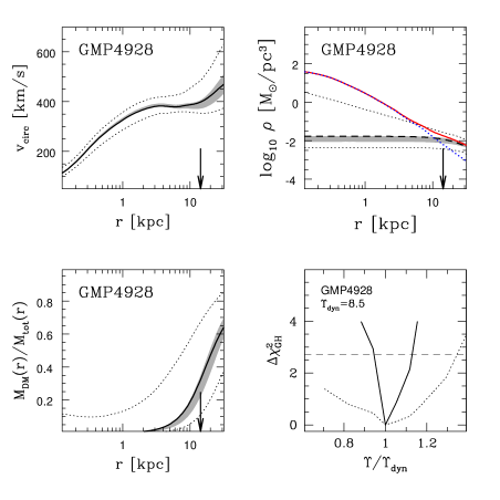
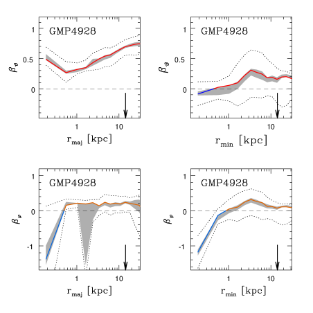
Figure 1: Comparison of confidence intervals with (shaded) and without (dotted) rescaling the $\chi^{2}$ (details in the text). Individual panels show circular velocity $v_{\mathrm{circ}}$, mass densities $\rho$ (stellar: blue/dotted, dark matter: black/dashed and total: red/solid), dark matter fraction $M_{\mathrm{DM}}/M$, $\chi^{2}_{\mathrm{GH}}$ (dotted without rescaling, solid with rescaling) and velocity anisotropies $\beta_{\vartheta}$ and $\beta_{\varphi}$ along major and minor-axis, respectively.

Among these models we determine the best-fit according to the lowest $\chi^{2}_{\mathrm{GH}}$, defined as

$$\chi^{2}_{\mathrm{GH}}\equiv\sum_{j=1}^{N_{\cal L}}\left[\left(\frac{v^{j}_{\mathrm{mod}}-v^{j}_{\mathrm{dat}}}{\Delta v^{j}_{\mathrm{dat}}}\right)^{2}+\left(\frac{\sigma^{j}_{\mathrm{mod}}-\sigma^{j}_{\mathrm{dat}}}{\Delta\sigma^{j}_{\mathrm{dat}}}\right)^{2}+\right.$$

$$\left.\left(\frac{H^{j}_{3,\mathrm{mod}}-H^{j}_{3,\mathrm{dat}}}{\Delta H^{j}_{3,\mathrm{dat}}}\right)^{2}+\left(\frac{H^{j}_{4,\mathrm{mod}}-H^{j}_{4,\mathrm{dat}}}{\Delta H^{j}_{4,\mathrm{dat}}}\right)^{2}\right].$$ (11)

Here, $v^{j}_{\mathrm{dat}}$ is the rotation according to the Gauss-Hermite parameterisation of the LOSVDs (other parameters analogously). A detailed discussion about the difference between $\chi^{2}_{\mathrm{GH}}$ and $\chi^{2}_{\mathrm{LOSVD}}$ can be found in Thomas et al. (2005).

Confidence intervals on model quantities are set by the corresponding minimum and maximum values obtained over all models within $\Delta\chi^{2}_{\mathrm{GH}}=1.1$ from the minimum $\chi^{2}_{\mathrm{GH}}$. The value of $\Delta\chi^{2}_{\mathrm{GH}}=1.1$ is slightly more conservative than the classical $\Delta\chi^{2}_{\mathrm{GH}}=1.0$ and has been derived by means of Monte-Carlo simulations (Thomas et al., 2005).

As a byproduct of the iterative technique to solve equation (5), we get – for each set of ($r_{c},v_{c},\Upsilon,i$), ($c,q,\Upsilon,i$) and ($\Upsilon,i$), respectively – orbit models for about $N_{\alpha}\approx 50$ different values of the regularisation parameter. This allows us to derive a best-fit model for each $\alpha_{i}$ and to explore the dependency of best-fit model parameters on $\alpha$ (cf. Sec. 9).

4 Modelling results

Modelling results are summarised in Tab. 2. In the remainder of this Section we collect some general notes on these results.

4.1 Goodness-of-fit

The goodness-of-fit obtained under the different assumptions about the overall mass distribution are given in columns (3), (7) and (11) of Tab. 2. Thereby

$$\chi^{2}_{\mathrm{SC}}\equiv\min\{\chi^{2}_{\mathrm{GH}}(\Upsilon,\,i)/N_{\mathrm{data}}\},$$ (12)

$$\chi^{2}_{\mathrm{LOG}}\equiv\min\{\chi^{2}_{\mathrm{GH}}(r_{c},\,v_{c},\,\Upsilon,\,i)/N_{\mathrm{data}}\}$$ (13)

and

$$\chi^{2}_{\mathrm{NFW}}\equiv\min\{\chi^{2}_{\mathrm{GH}}(c,\,q,\,\Upsilon,\,i)/N_{\mathrm{data}}\}$$ (14)

are minimised over all relevant mass parameters. Differences between models with and without dark matter are further discussed in Sec. 5.1. Here we only refer to the fact that our models are able to reproduce the observations with a $\chi^{2}_{\mathrm{GH}}$ per data point which is in many cases significantly smaller than unity. The largest deviations between model and data occur for the S0 GMP0756, possibly related to the low $H_{4}$ along the offset-axis, which are not followed by our models. Fits to some galaxies are as good as $\chi^{2}_{\mathrm{min}}\la 0.1$, where

$$\chi^{2}_{\mathrm{min}}\equiv\min\{\chi^{2}_{\mathrm{LOG}},\,\chi^{2}_{\mathrm{NFW}},\chi^{2}_{\mathrm{SC}}\}$$ (15)

describes the overall minimum of $\chi^{2}_{\mathrm{GH}}$ for a given galaxy. In many cases where $\chi^{2}_{\mathrm{min}}$ is particularly low, error bars of the observations are much larger than the point-to-point scatter of the data points. This concerns GMP5279, GMP2921, GMP4928, GMP5568 and GMP3958, where the observational errors are likely overestimated (see also the fits in App. A). In some other systems, like for example GMP0144, the error bars used in the modelling are rather large, because they also include side-to-side variations of the kinematics, which are often also larger than the point-to-point scatter on a given side of the galaxy. Thus, both effects might partly explain the low $\chi^{2}_{\mathrm{min}}$ of these galaxies.

Very low $\chi^{2}_{\mathrm{min}}$ raise the question whether confidence intervals of model properties calculated as described in Sec. 3.5 (and shown in Figs. 4, 5, 6 and 7 below) are overestimated. In cases where the observational errors are obviously too large it is reasonable to rescale them until $\chi^{2}_{\mathrm{min}}\approx 1$. In fact, this has been done for GMP5975 in Thomas et al. (2005), where error bars were scaled such that $\chi^{2}_{\mathrm{min}}\approx 0.7$. This value was determined from Monte-Carlo simulations of isotropic rotator models. To quantify the effect of rescaling, Fig. 1 exemplifies confidence intervals for one galaxy of the sample (GMP4928) once without rescaling the $\chi^{2}_{\mathrm{GH}}$ and once with rescaling all observational error bars to $\chi^{2}_{\mathrm{min}}=0.7$. As it can be seen, uncertainty regions shrink a lot after rescaling.

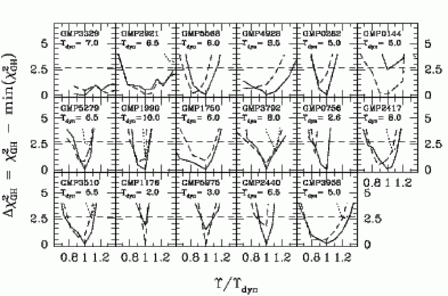
Figure 2: Confidence levels $\Delta\chi^{2}_{\mathrm{GH}}$ versus $\Upsilon$ (normalised to the best-fit $\Upsilon_{\mathrm{dyn}}$). Solid: logarithmic halos; dashed: NFW halos; dotted: mass follows light; horizontal dashed: 90 percent confidence limit. Where a dotted line is missing the self-consistent case is ruled out with more than 95 percent confidence (exception: GMP3329, where the best-fit $\Upsilon_{\mathrm{SC}}\approx 1.7\,\Upsilon_{\mathrm{dyn}}$ is outside the plotted region). From top-left to bottom-right galaxies are arranged in order of decreasing total mass inside $r_{\mathrm{eff}}$.

Globally rescaling the error-bars is not appropriate for all galaxies, however. Errors along the major-axis of GMP3792, for example, might be overestimated, but those along the minor-axis seem not. Moreover, in a case like GMP1750 slight minor-axis rotation – which cannot be fit with axisymmetric models – adds a constant to $\chi^{2}_{\mathrm{min}}$. Just rescaling to $\chi^{2}_{\mathrm{min}}\approx 0.7$ in all galaxies would introduce an artificial dependency of uncertainty regions on minor-axis rotation, which is not appropriate. In order to treat all galaxies of the sample homogeneously we do not rescale the $\chi^{2}_{\mathrm{GH}}$, but give the most conservative error-bars for our models. The corresponding confidence intervals may be interpreted as the maximal uncertainty on derived model quantities, while the shaded regions of Fig. 1 may be interpreted as lower limits for these uncertainties.

Fig. 2 shows the dependency of

$$\Delta\chi^{2}_{\mathrm{GH}}(\Upsilon)\equiv\chi^{2}_{\mathrm{GH}}(\Upsilon)-\mathrm{min}\,(\chi^{2}_{\mathrm{GH}}),$$ (16)

where $\mathrm{min}\,\chi^{2}_{\mathrm{GH}}\equiv\chi^{2}_{\mathrm{min}}\times N_{\mathrm{data}}$ (cf. equation 15) and $\chi^{2}_{\mathrm{GH}}(\Upsilon)$ is minimised over all NFW-fits, logarithmic-halo fits and self-consistent fits with the given $\Upsilon$. For all but one galaxy, we find a clear minimum in $\chi^{2}_{\mathrm{GH}}(\Upsilon)$. The exceptional case, GMP3329, is peculiar in many respects: (1) It is among the brightest galaxies of the sample and has a very large $r_{\mathrm{eff}}$. The data only cover the region inside $r\la r_{\mathrm{eff}}/2$. (2) The surface-brightness profile shows a break near $0.2-0.3\,r_{\mathrm{eff}}$ (cf. upper panel of Fig. 18). (3) At about the same projected distance from the centre the velocity dispersion dips and rises again at larger radii (cf. lower panel of Fig. 18). The poor constraints on the mass-to-light ratio in this system could be related to the poor data coverage. It might also be that GMP3329 is actually composed of two subcomponents. If these have different mass-to-light ratios $\Upsilon$, then the $\chi^{2}_{\mathrm{GH}}$-curve may have two corresponding local minima and the poor data coverage may smooth out these into a flat plateau. Finally, our modelling of GMP3329 may suffer from the Coma core being possibly not in dynamical equilibrium, as indicated by the kinematics of intra-cluster planetary nebulae (Gerhard et al., 2007).

4.2 Model inclinations

Most of the best-fit models are edge-on according to the last column of Tab. 2. This is surprising at first sight because if galaxies are oriented randomly then one would expect only about 6 out of 17 objects to have inclinations larger than $i\ga 70\degr$. Omitting the five systems for which only edge-on models were calculated (GMP0756, GMP1176, GMP1990, GMP2417 and GMP5975; cf. Sec. 3.1) and taking into account the uncertainties quoted in Tab. 2 there are 3 galaxies out of 11 where inclinations $i<70\degr$ are ruled out by our modelling (at the 68 percent confidence level). This is in good agreement with the expectation for random inclinations. Nevertheless, we now discuss a little more whether our modelling might be subject to a slight inclination bias.

First, one possible issue is that using the same regularisation for all galaxies might introduce a subtle bias towards edge-on configurations. Consider a rotating system: the lower the assumed inclination of the model the larger its intrinsic rotation needs to be in order to match the observations after projection. Thus, the system will be dynamically colder and its entropy will be lower. Turning the argument around: usage of a constant $\alpha$ enforces the same weight on entropy in the inclined model as in the edge-on model. Since the inclined model has to have lower entropy, however, its fit may be less good. This might drive models of rotating galaxies towards $i=90\degr$. We do not expect this to affect conclusions drawn from our modelling results strongly, because, as it has been argued in Sec. 3.1, error bars on intrinsic properties include in many cases models at different inclinations, even extreme cases. But it might drive the best-fit model to occur preferentially around $i=90\degr$.

Second, for face-on galaxies noise in the kinematics may be a source of bias towards edge-on models as well (Thomas et al., 2007b). It can cause rotation measurements $v\neq 0$ even for exactly face-on, axisymmetric galaxies. An edge-on model can in principle fit these $v\neq 0$, whereas face-on models necessarily obey $v\equiv 0$. Thus, everything else fitting equally well, the contribution of noise in $v$ to the $\chi^{2}$ would be smaller in edge-on than in face-on models. Since we have no clear candidate face-on galaxy in our sample we do not expect this issue to be relevant to the Coma sample, however.

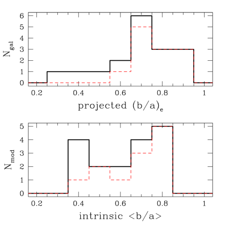
Figure 3: Top: histogram of apparent short-to-long axis ratios at $r_{\mathrm{eff}}$. Bottom: intrinsic best-fit short-to-long axis ratio $\langle b/a\rangle$ (averaged over $r/r_{\mathrm{eff}}\in[0.5,2.5]$). Black/solid: whole sample; red/dashed: without S0s.

The third thing to note is that galaxies for our sample may be not at random inclinations. The sample is designed to complement earlier studies on round galaxies and we explicitly selected flattened, rotating ellipticals and S0s to be fitted. The distribution of apparent axis-ratios $(b/a)_{e}\equiv 1-\epsilon_{e}$ (with $\epsilon_{e}$ from Tab. 1) is shown in the upper panel of Fig. 3. The sample exhibits a tail of highly flattened systems, which lacks, for example, in the distribution of bright galaxies with de-Vaucouleurs profiles in the Sloan Digital Sky Survey (Vincent & Ryden, 2005). This tail is produced by the S0 galaxies in our sample and clearly shows that the sample as a whole is biased towards flattened systems. The ellipticity distribution of those galaxies that are classified as ellipticals in Tab. 1 (dashed line in Fig. 3) is still shifted slightly towards higher ellipticities with respect to the bright ellipticals of Vincent & Ryden (2005). In combination with the lack of round objects in our sample, this indicates that even our 11 ordinary ellipticals are slightly biased, but the sample is too small for a definite appraisal.

Fourth, even assuming our sample galaxies are at random inclinations and that the first two just discussed points are irrelevant (regularisation and noise) and that inclinations can be reconstructed uniquely from ideal data with ideal models then we still could be faced with a slight bias in our models: as it has been described in Sec. 3.1 we do not probe a fine grid in inclinations but look for extreme cases. Our models provide for each galaxy only the choice between edge-on or intrinsically E5/E7, respectively. Since an intrinsic E5/E7 shape is a rather extreme assumption this might drive the modelling towards the edge-on option as well.

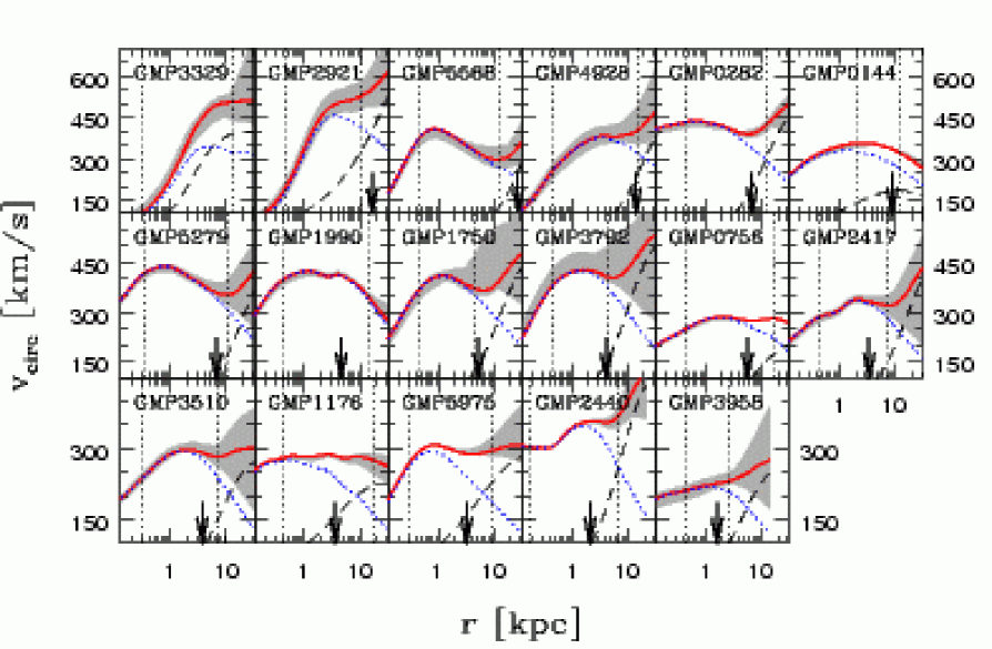
Figure 4: Compilation of circular velocity curves. Thick/red: luminous+dark (68 per cent confidence region shaded); dotted/blue: luminous only; dashed: dark matter only; vertical dotted lines: boundaries of kinematical data; arrows denote the effective radius $r_{\mathrm{eff}}$. From top-left to bottom-right galaxies are arranged in order of decreasing total mass inside $r_{\mathrm{eff}}$.

The distribution of intrinsic axis ratios of the Coma models is shown in the lower panel of Fig. 3. It peaks at $b/a=0.8$, consistent with deprojections of the frequency function of elliptical galaxy apparent flattenings (Tremblay & Merritt, 1996; Vincent & Ryden, 2005). Compared with these studies, the distribution in the lower panel of Fig. 3 has relatively more galaxies on the flatter side of the peak and relatively fewer galaxies on the rounder side. Now, if the modelling would be subject to a strong bias towards $i\to 90\degr$ then we would expect the opposite: an overestimation of intrinsically roundish galaxies. Thus, the lower panel of Fig. 3 argues against a strong modelling bias towards high inclinations. However, the argument is not conclusive, because the sample itself maybe biased against apparently round galaxies. This could partly compensate for an inclination bias in the modelling.

In conclusion, although there might be a slight inclination bias in the modelling and/or the sample galaxies, Fig. 3 reveals that either this bias is not very strong, or that modelling and sample biases roughly counterbalance each other.

5 Luminous and dark matter distribution

Now we discuss the distribution of luminous and dark matter in the Coma models.

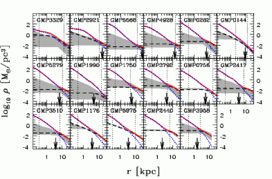
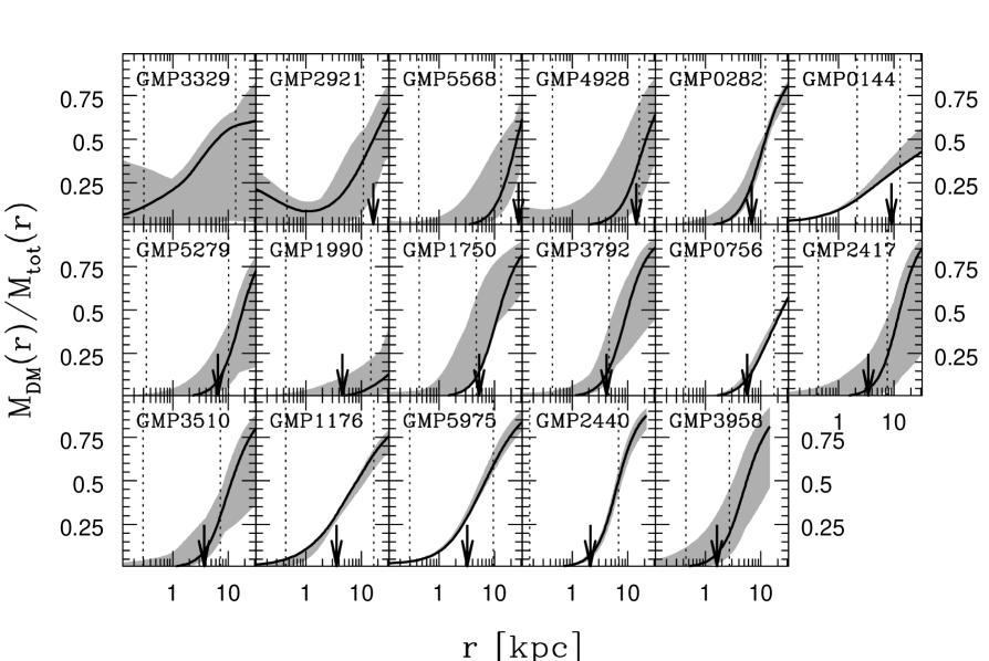
Figure 5: Top: spherically averaged mass densities. Red (solid): total mass; blue (dotted): luminous mass; black (dashed): dark matter with errors (shaded). Bottom: corresponding spherically averaged dark matter fractions with 68 percent confidence regions. Vertical dotted lines and arrows as in Fig. 4.

5.1 Does mass follow light?

According to Tab. 2, the best-fit model of each galaxy contains a dark matter halo. Column (14) of the table states that eight galaxies have at least a two sigma detection of a dark matter halo (GMP0282, GMP0756, GMP1176, GMP1750, GMP2440, GMP4928, GMP5568 and GMP5975). The best fitting models with and without dark matter, respectively, are compared to the kinematic data in App. A. From this comparison it follows that models without a halo obviously fail to reproduce the kinematic data for the above mentioned galaxies. The evidence for dark matter thereby comes mostly from the innermost and outermost kinematic data points: without dark matter, the energy of the models is too low, when compared to the data at large radii and too high, when compared to the central data (for example illustrated by the dispersion profile of GMP5975). The reason for the differences at small radii is likely that part of the missing outer mass in models without a halo is compensated for by a larger mass-to-light ratio (cf. Sec. 5.5). This, in turn, causes an increase of the central mass and central velocity dispersion, respectively. In GMP1750 the dispersion profile without dark matter fits systematically worse than the one with dark matter at all radii. Concerning GMP5568, the dispersion along one of the offset-slits is particularly large, larger than in all other slits. It is not entirely clear if these large dispersions are real. If not, then they erroneously increase the evidence for dark matter. However, because the error-bars of the corresponding data points are very large, these dispersions are not the dominant driver for the dark halo detection in GMP5568.

In the rest of the sample the detection of dark matter – if at all – is more of statistical nature. Models with and without dark matter for GMP0144 and GMP2921 differ in a similar fashion as those of GMP1750. For GMP3510, GMP3958 and GMP5279 small differences between models with and without dark matter can be seen at the last kinematic data points, but the formal significance for dark matter is less than 90 percent. We believe that the statistical significance for dark matter in these five cases is underestimated due to our very conservative error estimates.

In the four remaining objects GMP1990, GMP2417, GMP3329 and GMP3792 the evidence for dark matter is generally low. Poor evidence for dark matter in GMP3329 maybe related to the overall poor constraints that the measured kinematics put on its mass-to-light ratio (cf. Sec. 4.1). GMP1990 is consistent with the assumption that mass follows light.

Our sample thus roughly divides into three categories: (1) galaxies that are clearly inconsistent with a constant mass-to-light ratio (8 galaxies out of 17). (2) Cases where models with and without a dark halo differ systematically, but where the formal evidence for a dark halo is less than two sigma (5 galaxies). In these cases we expect that our very conservative error bars lead to an underestimation of the dark matter detection. (3) Systems in which the evidence for dark matter is generally weak (4 galaxies).

Models and data of some galaxies with a clear dark halo detection still differ systematically in the outer parts (e.g. GMP0756, GMP1176 and GMP5975). Decreasing the weight on regularisation reduces these differences. However, according to the discussion of Sec. 3.4 we do not expect that we have significantly over-regularised our models. Even in case we would have, the derived halos of these systems do not depend much on the choice of the regularisation parameter, such that conclusions upon the masses of these galaxies are robust (cf. Sec. 9). It might be possible that differences between models and data are related to changes in the stellar population, that other our adopted halo profiles are not appropriate for these systems, or that the corresponding outer regions are not in equilibrium or not axisymmetric. We plan further investigations of these topics for future publications.

5.2 Circular velocity curves

Fig. 4 shows the best-fit circular velocity curves for the Coma galaxies. The shapes of the curves vary from cases with two local extrema (e.g. GMP5279) to a case of monotonic increase (GMP3958). The sample provides examples of rising as well as falling outer circular-velocity curves. Flattened, rotating galaxies have fairly flat circular velocity curves beyond the central rise (less than 10 percent variation up to the last kinematic data point in GMP0282, GMP0756, GMP2417, GMP3510, GMP1176 and GMP5975).

5.3 Mass densities and dark matter fractions

Spherically averaged density profiles of all Coma galaxies are surveyed in the top panel of Fig. 5. The luminosity distribution of most galaxies shows a power-law core that smoothly joins with the outer light-distribution. Towards the most luminous galaxies the central slope of the luminosity distribution flattens out (GMP3329 and GMP2921). The inner breaks in the light profiles of GMP1990 ($r\approx 2\,\mathrm{kpc}$), GMP2417 ($r\approx 1\,\mathrm{kpc}$) and GMP2440 ($r\approx 0.3\,\mathrm{kpc}$) originate from prominent dust features.

The central regions are dominated by luminous matter. Halo densities in the centre are at least one order of magnitude lower than stellar mass densities – independently of the halo profile being either of the logarithmic or of the NFW type. The radius where dark and luminous mass densities equalise is inside the kinematically sampled region of each galaxy. In some galaxies the transition from the luminous inner parts to the dark matter dominated outskirts is very smooth (for example GMP0756, GMP1176, GMP5975). The corresponding dark halo components are relatively concentrated (NFW halos) and the circular velocity curves are fairly flat. In other galaxies the transition is marked by a break in the total mass profile and a dip in $v_{\mathrm{circ}}$ (for example GMP0282). We will come back to these different circular velocity curve shapes in Thomas et al. (2007a, in preparation).

Dark matter fractions of the best-fit Coma models are shown in the bottom panel of Fig. 5. In most galaxies 10 to 50 percent of the mass inside $r_{\mathrm{eff}}$ is dark.

5.4 NFW or logarithmic halos?

The evidence for or against logarithmic and NFW halos is summarised in column (13) of Tab. 2. The majority of best-fit models (13 out of 17) is obtained with logarithmic halos. However, the significance for one or the other halo profile providing the better fit is in most cases low. As already implied by the approximate flatness of the circular velocity curves, the overall effect of the halo component is to keep the outer logarithmic slope of the total mass density around $-2$ (i.e. the case of an exactly constant $v_{\mathrm{circ}}$). This can be achieved either with logarithmic halos (asymptotically) or with suitably scaled NFW halos (over a finite radial range around the scaling radius). Differences in the profiles’ inner slopes seem to play a minor role, perhaps because the inner mass profile turns out to closely follow the light profile. If elliptical galaxy circular velocity curves are roughly flat over a very extended radial range, then NFW fits will break down at some point. With the data at hand no clear decision in favour of one of the two profiles can be made.

Most of the best-fit NFW-models are obtained with a flattened halo. Since we cannot significantly discriminate between NFW and LOG-halos, firm statements about the flattening of the halos are not possible.

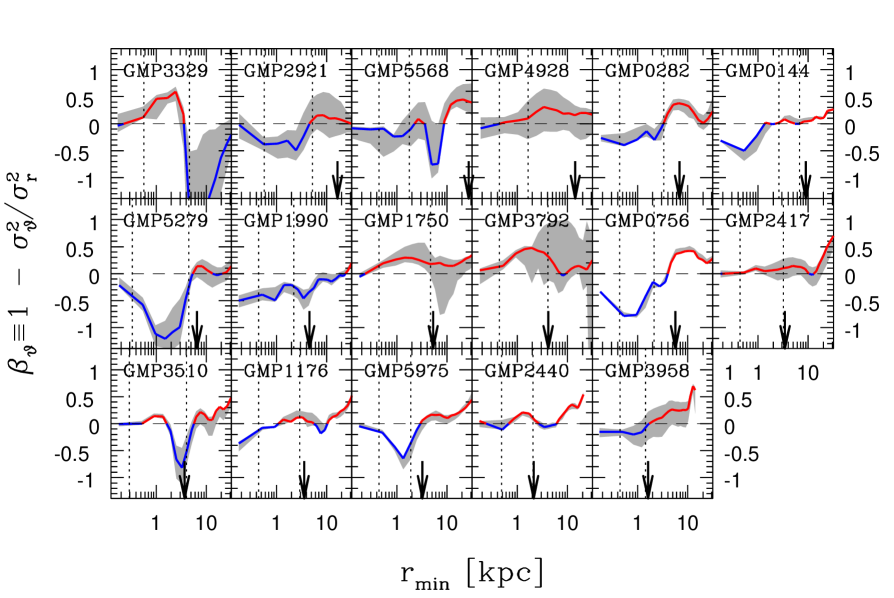
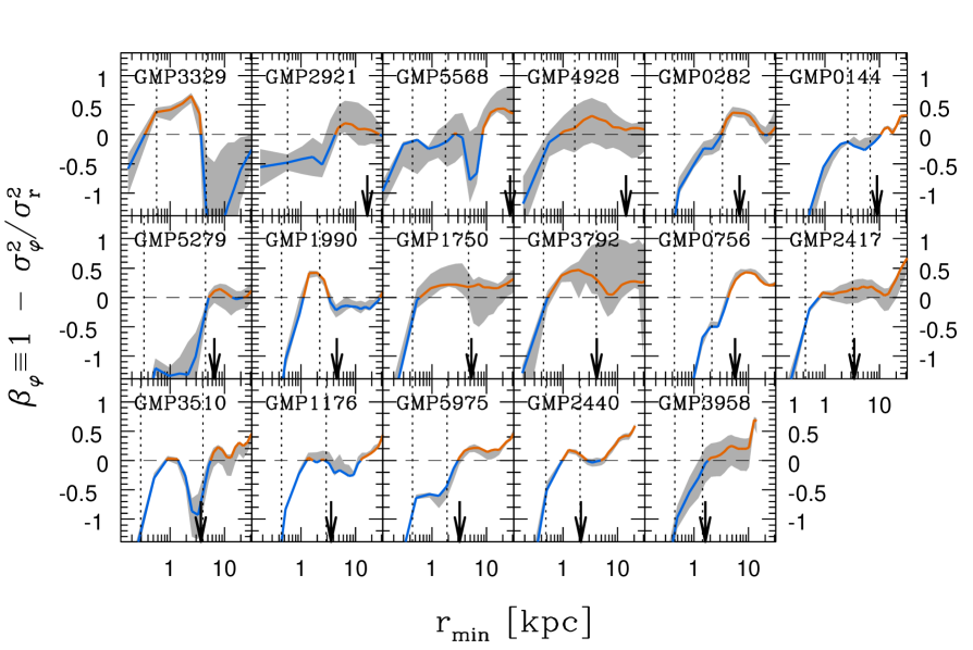
Figure 6: Minor-axis anisotropy profiles. Top: meridional anisotropy $\beta_{\vartheta}$; bottom: azimuthal anisotropy $\beta_{\varphi}$; solid: best-fit models (in the colour-version radial anisotropy is highlighted in red, tangential anisotropy in blue); shaded: 68 percent confidence region; dotted: region with kinematic data; arrows: $r_{\mathrm{eff}}$.

5.5 The fraction of mass that follows the light

From Tab. 2 it can be taken that mass-to-light ratios $\Upsilon_{\mathrm{SC}}$ of self-consistent models are on average ($17\pm 10$) percent larger than those of models with a dark matter halo. Concerning the difference between logarithmic and NFW halos, the best-fit $\Upsilon_{\mathrm{NFW}}$ is generally equal or lower than the corresponding $\Upsilon_{\mathrm{LOG}}$.

6 Velocity Anisotropy

Having explored the mass structure of the models we next focus on their dynamics. In this section we will consider the velocity anisotropies defined in equations (9) and (10), respectively.

The discussion will be restricted to the minor-axis and major-axis bins of the Schwarzschild models, respectively. Each galaxy is covered by kinematical observations along at least these axes and the internal orbital structure is best constrained there.

6.1 The polar region

Fig. 6 surveys velocity anisotropy profiles along the intrinsic minor-axis of the Coma galaxy sample. According to axial symmetry $\beta_{\vartheta}\equiv\beta_{\varphi}$ holds directly on the symmetry axis. Hence, the upper and lower panel of Fig. 6 are overall very similar. The minor-axis bins of the models, however, form a cone with opening angle $\Delta\vartheta=25\degr$ around the $z$-axis. Thus, they include regions off the symmetry axis, where the equivalence between azimuthal and meridional dispersions does not hold, such that $\beta_{\vartheta}$ and $\beta_{\varphi}$ in Fig. 6 are not identical.

In Fig. 6 the very central anisotropies should not be regarded as reliable. Firstly, because the central bins are affected from incomplete orbit sampling, resulting in artificially large azimuthal dispersions (Thomas et al., 2004). Secondly, for numerical reasons the innermost bin is not resolved in $\vartheta$, but averaged over all $\vartheta\in[0\degr,\,90\degr]$.

In the spatial region with kinematical data the Coma galaxies offer different degrees of minor-axis anisotropy, from strongly tangential (GMP5279) to moderately radial (GMP3792). Towards the centre $\beta_{\vartheta}\rightarrow 0$, while $\beta_{\varphi}$ becomes negative (most likely due to the incomplete orbit sampling). Going outward, many but not all galaxies exhibit a gradual change in dynamical structure, often in form of a minimum or maximum in $\beta$. Around the last data point most models are isotropic. The most radial system is GMP3792.

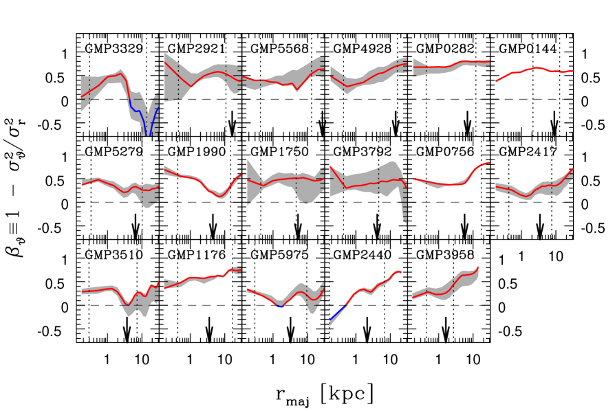
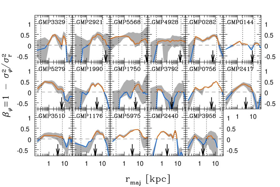
Figure 7: As Fig. 6, but for the major axis.

6.2 The equatorial plane

Velocity anisotropy profiles in the equatorial plane are shown in Fig. 7. Note that unlike along the minor-axis axial symmetry does not imply any relationship between $\beta_{\varphi}$ and $\beta_{\vartheta}$ at low latitudes.

Meridional anisotropy.

Contrasting the situation around the poles, almost no galaxy exhibits tangential anisotropy $\beta_{\vartheta}<0$. Apart from the peculiar object GMP3329 (cf. Sec. 4.1) all galaxies have $\beta_{\vartheta}>0$ over the kinematically sampled radial range. The average $\beta_{\vartheta}$ turns out to be related to the intrinsic flattening of the galaxies (Thomas et al. 2007a, in preparation). Uncertainties on the intrinsic shape therefore propagate into uncertainties on $\beta_{\vartheta}$. As it has been stated in Sec. 3.1, in many cases it is not possible to distinguish between different inclinations with high significance. Hence, intrinsic shapes are likewise poorly constrained and the uncertainties on $\beta_{\vartheta}$ become large. A typical example is GMP3792: the best-fit inclination is $i=60\degr$ and requires a relatively flattened intrinsic configuration with large $\beta_{\vartheta}$. However, models at higher as well as lower $i$ are within the 68 percent confidence region. Consequently, the shaded area includes also models with different flattening and $\beta_{\vartheta}$.

Figure 8: Short-axis anisotropy against minor-axis $H_{4}$. The line in the upper panel shows a linear fit (quoted in the panel).

Azimuthal anisotropy.

More diversity than in $\beta_{\vartheta}$ is offered by azimuthal velocities. In GMP3792, for example, $\beta_{\varphi}<0$ suggests that the system may be composed of two flattened subsystems with low net angular momentum, causing large $\varphi$-motions. GMP3510, GMP3958 and GMP0144 are relatively isotropic ($\sigma_{r}\approx\sigma_{\varphi}$) over the kinematically sampled spatial region. GMP5279, instead, offers $\beta_{\vartheta}\approx\beta_{\varphi}>0$, implying $\sigma_{r}>\sigma_{\varphi}$ and $\sigma_{r}>\sigma_{\vartheta}$ over the region with data.

6.3 Relations between anisotropy and observed kinematics

The intrinsic short-axis velocity anisotropies are closely related to the observed (local) $H_{4}$. This can be taken from Fig. 8, where for each (projected) radius $R$ with a measurement of $H_{4}$ the local $H_{4}(R)$ is plotted against the internal anisotropy $\beta(r=R)$ at the same radius. Internal radii $r$ have not been corrected for inclination since most models are edge-on (cf. Sec. 4.2). From the figure a tight correlation of $\beta_{\vartheta}$ with $H_{4}$ follows (quoted in the plot): the smaller $H_{4}$, the more tangentially anisotropic the model. A similar trend occurs between $\beta_{\varphi}$ and $H_{4}$ (lower panel). This reflects that $\beta_{\vartheta}\approx\beta_{\varphi}$ around the symmetry axis (see above).

Comparable trends between $\beta$ and $H_{4}$ have also been found in spherical models (e.g. Gerhard 1993; Magorrian & Ballantyne 2001). The similarity between spherical models on the one hand and the polar region of axisymmetric models on the other might be connected to the fact that in both cases $\sigma_{\varphi}=\sigma_{\vartheta}$. In other words, effectively there is only one degree of freedom in the stellar anisotropy ($\beta_{\varphi}=\beta_{\vartheta}$) and, if the potential is fixed, there must be a close relationship between $\beta$ and the shape of the LOSVD (as measured by $H_{4}$). Experiments with spherical models indicate that the dependency of $H_{4}$ on the potential is weaker than its variation with $\beta$ (e.g. Gerhard 1993; Magorrian & Ballantyne 2001). If the same holds for axisymmetric potentials, then this would explain why along the polar axis of axisymmetric models $\beta$ depends in about the same way on $H_{4}$ as in spherical models. Note, however, that our Schwarzschild models provide many more internal degrees of freedom than the smooth spherical models considered by Gerhard (1993) and Magorrian & Ballantyne (2001). This becomes apparent when the influence of regularisation on the fit is lowered and the scatter around the relation shown in Fig. 8 increases (cf. Sec. 9.2).

In contrast to the polar region, no tight correlation between $H_{4}$ and velocity anisotropy is found around the equatorial plane (cf. Fig. 9). This holds especially for $\beta_{\vartheta}$, whereas there is a slight trend of $\beta_{\varphi}$ to increase with $H_{4}$. For comparison, a linear fit is shown in the lower panel. A detailed investigation of the orbital structure will be presented in another paper (Thomas et al. 2007a, in preparation).

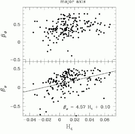
Figure 9: As Fig. 8, but for the major-axis.

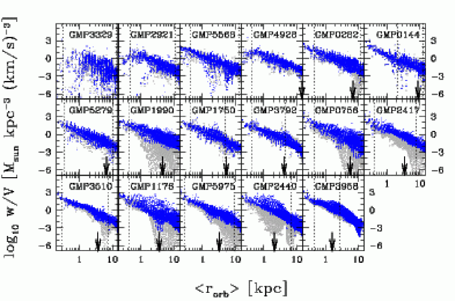
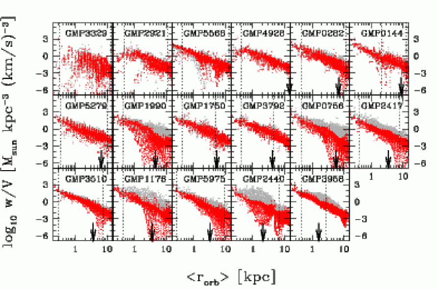
Figure 10: Luminous matter phase-space densities. Top: prograde orbits are highlighted (blue); bottom: retrograde orbits are highlighted (red); vertical dotted lines: boundaries of kinematical data; arrows: $r_{\mathrm{eff}}$.

7 Phase-space distribution function of the stars

A more fundamental quantity related to a stellar dynamical system than its anisotropy is its phase-space distribution function $f$. It describes the density of stars in phase-space and offers the most detailed and comprehensive view on its dynamical state. For stationary systems the DF is a function of the (isolating) integrals of motion and, thus, constant along individual orbits (Jeans theorem; e.g. Binney & Tremaine 1987). To be considered in axisymmetric potentials are the energy $E$, angular momentum $L_{z}$ along the axis of symmetry and, in most astrophysically relevant potentials, the so-called third integral $I_{3}$. To be physically meaningful the DF has to obey the further condition that it is positive everywhere. In Schwarzschild models the constancy of the DF along orbits is explicitly taken into account during the orbit integration. Its positive definiteness is guaranteed as long as the orbital weights $w_{i}$ are positive (cf. equation 7). In other words, the very existence of our Schwarzschild models ensures that the luminous component of the model is stationary and physically meaningful (positive density).

A detailed investigation of the full dependency of the DF on all integrals of motion and its connection to stellar population properties will be the subject of another publication (Thomas et al. 2007a, in preparation). Here we only consider some general properties of the DF. For this purpose it is convenient to define a mean orbital radius

$$\langle r_{\mathrm{orb}}\rangle_{i}\equiv\sum_{k}\frac{\Delta t^{k}_{i}}{T_{i}}r^{k}_{i},$$ (17)

where $T_{i}$ is the total integration time of orbit $i$ and $r^{k}_{i}$ is its radius at time-step $k$ (lasting $\Delta t^{k}_{i}$). In rough terms $\langle r_{\mathrm{orb}}\rangle$ can be interpreted as a measure of the orbital binding energy.

Fig. 10 surveys the DFs of all 17 Coma galaxies. Each dot represents the phase-space density of a single orbit. To roughly trace the angular-momentum dependency of the DF prograde orbits with $L_{z}>0$ are highlighted in the top panel and retrograde orbits ($L_{z}<0$) are highlighted in the bottom one.

The figure shows that with decreasing galaxy mass differences between prograde and retrograde orbits in phase-space become more significant. This partly reflects an increasing importance of rotation in lower mass galaxies of our sample. Often, the highest phase-space densities of prograde orbits are nearly constant over some radial region (e.g. GMP3958 around $r_{\mathrm{eff}}$, GMP2440 inside $r\la r_{\mathrm{eff}}$). In many, but not all, rotating galaxies the dominance of prograde orbits comes along with a strong depression of retrograde orbits. In the outer parts of GMP5975, for example, retrograde orbits have phase-space densities up to 10 orders of magnitude smaller than prograde orbits. Such low-density orbits can actually be regarded as being absent in the models (Thomas et al., 2005). Concerning the significance of this depopulation it is interesting to note that in case of GMP5975 it was originally found in models based on major and minor-axis data only (Thomas et al., 2005), but remains almost unchanged in our new models including additional kinematical information along a diagonal axis (cf. Sec. 2). The depopulation of retrograde orbits cannot be a general modelling artifact since it does not appear in all rotating galaxies. A counter-example is the least-massive object, GMP3958: it rotates but does not show a strong depression of retrograde orbits in its outer parts.

One galaxy of the sample, GMP5568, hosts a counter-rotating central disk (Mehlert et al., 1998), which shows up by a dominance of retrograde orbits around $\langle r_{\mathrm{orb}}\rangle\approx 1\,\mathrm{kpc}$ and $w/V\approx 10\,M_{\odot}/\mathrm{pc}^{3}/(\mathrm{km}/\mathrm{s})^{3}$ in Fig. 10. In most rotating galaxies the majority of retrograde orbits follows approximately a power-law like straight line (e.g. GMP3958, GMP2417). Retrograde orbits in GMP1990 follow such a power-law like distribution only outside $r_{\mathrm{eff}}$. Near the centre of the galaxy retrograde orbits exhibit some excess density, compared to a power-law extrapolation of the behaviour outside $r_{\mathrm{eff}}$. This may reflect a faint inner counter-rotating sub-component, although unlike in GMP5568, prograde orbits always dominate in GMP1990 (and the observed sense of rotation is the same at all radii).

In some galaxy models orbital phase-space densities are more spread than in others: for example the DFs of GMP3329 and GMP5568 look particularly noisy. In case of GMP3329 its peculiar kinematics, already discussed in Sec. 5.1, may be responsible for the distorted phase-space distribution of orbits.

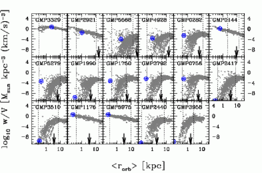
Figure 11: As Fig. 10, but for dark matter. No distinction between prograde and retrograde orbits is made (see text for details); large (blue) symbols: average phase-density of all orbits with $\langle r_{\mathrm{orb}}\rangle<0.1\,r_{\mathrm{eff}}$.

8 Phase-space distribution function of dark matter

So far we have only considered the phase-space distribution function of the luminous component of our models. To ensure that these models are physically meaningful we also need the dark halos to be supported by an everywhere positive phase-space distribution function. Without the baryons present, the existence of DFs for our halo profiles is known. In case of NFW-halos it follows trivially from the fact that they arise in $N$-body simulations and DFs for LOG-halos have been constructed explicitly by Evans (1993). With a significant contribution of baryons (or any other component) to the overall gravitational potential, the existence of these DFs is no longer guaranteed, however. For example, if a cored halo (central logarithmic density slope $\gamma=0$) is embedded in a cuspy baryonic component ($\gamma=-1$) and if the core radius exceeds a critical limit around $r_{C}\ga 3\,r_{\mathrm{eff}}$, then central phase-space densities become negative in isotropic or radially anisotropic systems (Ciotti & Pellegrini, 1992; Ciotti, 1999). In contrast, a cuspy halo can always be supported (Ciotti, 1996). Thus, the existence of a plausible halo DF for our LOG-halos, which often have core radii near or beyond the critical limit (cf. Tabs. 1 and 2) is not obvious. The main goal of this section is to investigate whether we can find a positive definite DF for all our best-fit models, or whether the phase-space analysis rules out some of our halo profiles.

8.1 Construction and existence of the halo distribution function

Our modelling machinery allows to construct a DF for dark matter in an analogous way as for luminous matter: by solving equation (5) with an orbit superposition. The only difference to the calculation of the luminous matter orbit superposition is that now the dark matter density profile is used as the boundary condition and not the deprojected light-profile $\nu$. In addition, since we lack of any kinematic information about the hypothetical halo constituents we set $\alpha=0$ in equation (5) and maximise the entropy of the orbits. For our goal of finding at least one positive definite DF this does not imply any loss of generality.

Within the numerical resolution of our orbit models we find indeed orbit superpositions with positive orbital weights $w_{i}>0$ that allow to reconstruct the halo density profile in each case. The corresponding DFs are stationary by construction and positive everywhere. The fact that we even find positive definite DFs for those LOG-halos that are beyond the above cited critical core-radius can have several reasons: our models are slightly different from the ones used in Ciotti (1999) (different radial run in outer parts, baryonic component flattened in our case). In addition, our orbit superpositions can well produce tangential anisotropy, which helps to maintain a positive DF. Finally, our orbit models have a finite resolution. We cannot exclude that reconstructing the halo density with higher resolution would force some orbital weights to become negative.

8.2 Differences between NFW and LOG-halos

Apart from the mere existence, there are significant differences in the derived DFs, however. This can be taken from plots of the halo DFs in Fig. 11. NFW-halo DFs (GMP2921, GMP0144, GMP1176 and GMP5975) are monotonic with respect to $\langle r_{\mathrm{orb}}\rangle$ and regular. The high degree of regularity (compared to the corresponding luminous matter DFs) reflects the maximisation of entropy, whereas noise in the stellar kinematics and sub-structuring of stars in phase-space tend to broaden the stellar DF (cf. Sec. 7) .

DFs of LOG-halos exhibit a drop of central phase-space density, as predicted by Ciotti (1999). In GMP3329, where the halo is very concentrated, the drop is rather gentle. With increasing core-radius the drop becomes more substantial. In addition, the noise in the DF increases with increasing core radius. Such disturbances in the DF, even though we maximise the entropy, indicate that a fine-tuning of the orbits is necessary for large core-radii to be supported by a positive-definite DF. This, and the non-monotonic dependency of orbital phase-space densities on $\langle r_{\mathrm{orb}}\rangle$ could imply that the corresponding DFs and, thus, also the spatial density profiles are unstable. If this is indeed the case, then the phase-space analysis would provide a strong argument against large-cored halo profiles, independent from the kinematic fits. Of course, the halo DFs shown in Fig. 11 are not unique, as stated above: the models have no access to the orbit distribution in the halo, apart from those constraints coming from the shape of the density-profile alone. Details of the DFs in Fig. 11 are therefore physically meaningless. However, that the entropy maximisation does not yield smooth DFs for LOG-halos with large cores suggests that – independent from our ignorance about the details of the orbit distribution – smooth dark matter DFs in the corresponding baryonic potential wells are unlikely.

In any case, a systematic stability analysis is out of the scope of this paper. What we can conclude here is, that based on the kinematic fits and based on the mere existence of a positive definite halo DF, we cannot rule out one or the other halo profile with our orbit models. Shape and structure of LOG-halo DFs make them the less likely option, however.

8.3 Central dark matter density

According to Sec. 5.3 the central density of dark matter is often orders of magnitudes lower than the luminous mass density. This suggests that it is in many cases weakly constrained. Could it be even lower than in LOG-halos? According to the above phase-space analysis this seems unlikely, because lower central densities would most likely augment the disturbances of the halo DF. Thus, the central spatial dark matter densities of our LOG-halos are likely lower limits to the true central dark matter densities.

8.4 Central dark matter phase-space density

From the dark matter DFs of Fig. 11 we have also calculated a mean central phase-space density

$$f_{h}\equiv\left(\frac{\sum w_{i}}{\sum V_{i}}\right)_{0.1},$$ (18)

where the sums on the right hand side are intended to comprise all orbits with $\langle r_{\mathrm{orb}}\rangle<0.1\,r_{\mathrm{eff}}$. These central phase-space densities are flagged in Fig. 11 by the large symbols. Comparison with Fig. 10 shows that central dark matter phase-space densities are particularly low in systems with strong rotation. Exceptions are GMP1176 and GMP5975 with their NFW halos.

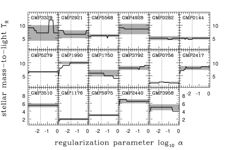
Figure 12: Best-fit $\Upsilon_{\mathrm{dyn}}$ versus regularisation parameter $\alpha$. Dotted line: $\alpha=0.02$, the regularisation adopted for the best-fit models; shaded: one sigma confidence region for $\alpha=0.02$.

The uncertainty in the dark-halo DF related to our ignorance about dark matter kinematics of course affects $f_{h}$. According to our above discussion the drop in LOG-halo DFs seems a feature connected to the density profile, though, and we do not expect that reasonably isotropic or radially anisotropic LOG-halo DFs exist for which $f_{h}$ increases by orders of magnitude. Thus, although $f_{h}$ is subject to many uncertainties, it is likely good as an order of magnitude estimation for the central dark matter phase-space density connected with the mass decomposition made in Sec. 3.2.

9 Regularisation

As it has been discussed in Sec. 3.4 the same regularisation $\alpha=0.02$ is adopted for all Coma galaxies. In the following we will discuss the dependency of our modelling results on the choice of $\alpha$.

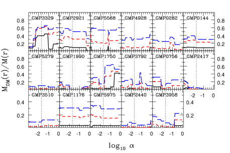
Figure 13: Dark matter fractions at $0.1\,r_{\mathrm{eff}}$ (black/solid), $0.5\,r_{\mathrm{eff}}$ (red/short-dashed) and $1.0\,r_{\mathrm{eff}}$ (blue/long-dashed) versus regularisation parameter $\alpha$. Vertical dotted lines: $\alpha=0.02$.

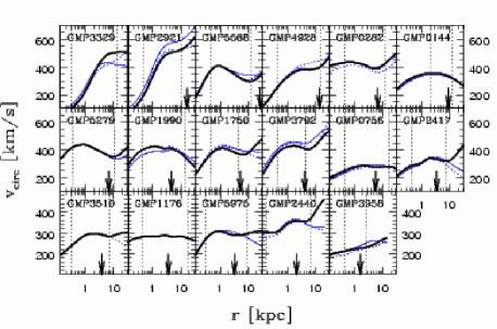
Figure 14: Best-fit circular velocity curves for different values of the regularisation parameter: $\alpha=0.001$ (blue, solid), $\alpha=2.7$ (blue, dotted) and $\alpha=0.02$ (black, solid).

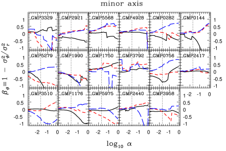
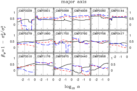
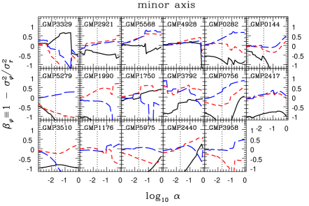
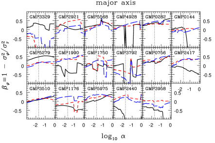
Figure 15: Best-fit anisotropy at $0.1\,r_{\mathrm{eff}}$ (black/solid), $0.5\,r_{\mathrm{eff}}$ (red/short-dashed) and $1.0\,r_{\mathrm{eff}}$ (blue/long-dashed); top: meridional anisotropy, bottom: azimuthal anisotropy; left: minor-axis, right: major-axis; vertical dotted lines: $\alpha=0.02$.

9.1 The influence of regularisation on model masses

Fig. 12 surveys the best-fit stellar mass-to-light ratios $\Upsilon_{\mathrm{dyn}}$ over the regularisation interval $\alpha\in[10^{-5},3]$. Two conclusions can be drawn from the figure. First, no systematic trend of $\Upsilon_{\mathrm{dyn}}$ with $\alpha$ is noticeable. In GMP1990, for example, $\Upsilon_{\mathrm{dyn}}$ increases with $\alpha$, while in GMP1750 it decreases. Second, in most of the sample galaxies the weight on regularisation has barely any effect on $\Upsilon_{\mathrm{dyn}}$ (e.g. GMP5568, GMP0282, GMP0144, GMP5279, GMP2417, GMP3510, GMP1176, GMP5975, GMP2440).

The best-fit dark matter fractions at three representative radii are shown in Fig. 13 as a function of $\alpha$. As could have been expected, the dark matter fraction and $\Upsilon_{\mathrm{dyn}}$ are correlated: in most cases where $\Upsilon_{\mathrm{dyn}}$, say, increases, the dark matter fraction decreases (and vice versa). Since there is no systematic trend of $\Upsilon_{\mathrm{dyn}}$ with $\alpha$ it follows that there is also no systematic trend of the dark matter fraction with $\alpha$. Moreover, the variation of dark matter fractions with $\alpha$ is within the quoted error budget of Fig. 5.

Finally, Fig. 14 shows circular velocity curves for three different values of $\alpha$. The influence of $\alpha$ on the shape of the circular velocity curve is weak. Only in a few systems the general shape of the circular velocity curve changes with $\alpha$ (for example GMP3510). These changes occur mostly outside the region covered by kinematic data, however.

9.2 The influence of regularisation on model kinematics

Now to the influence of $\alpha$ on the derived velocity anisotropies: the left panels of Fig. 15 show best-fit meridional and azimuthal velocity anisotropies at three representative radii as a function of $\alpha$. The figures indicate that maximum entropy fits ($\alpha\rightarrow 0$) yield isotropy along the minor-axis. Lowering the weight on regularisation generally increases the anisotropy – the absolute value of $\beta$ – in the models, as could have been expected. There is no specific trend of $\beta$ with $\alpha$: some systems gain more tangential anisotropy with increasing $\alpha$ (for example GMP5279), while others become more radial (for example GMP0756). In most cases the dependency of $\beta$ on $\alpha$ is monotonic and $\beta(\alpha)$ does not change sign. In other words, whether or not a galaxy model is tangentially or radially anisotropic does not depend on $\alpha$. Only the exact degree of anisotropy changes with $\alpha$.

Major-axis velocity anisotropies are plotted on the right hand side of Fig. 15. In contrast to the minor-axis case there is no trend of $\beta_{\vartheta}\to 0$ for $\alpha\to 0$. Variations of intrinsic velocity anisotropies with $\alpha$ are slightly weaker along the equator than they are along the minor-axis. Since the trend of $\beta$ with $\alpha$ is again monotonic and sign preserving in most cases, the general property of a galaxy to be radially or tangentially anisotropic is insensitive to the particular choice of $\alpha$.

From the top-left panel of Fig. 15 it is clear that the relation between (the $\alpha$-dependent) anisotropy and (the $\alpha$-independent) $H_{4}$ described in Sec. 6 must change with different amounts of regularisation in the models. This is illustrated in Fig. 16, which repeats the upper panel of Fig. 8 for two different values of $\alpha$. The consequences of stronger regularisation are displayed in the top panel, while weaker regularisation leads to the distribution shown in the bottom panel. For comparison the linear fit from Fig. 8 is shown by the dashed line. Increasing the weight on regularisation makes the correlation tighter, but does not alter the slope. With less regularisation the scatter increases, because models start to fit the noise in the data. The mean relation is in any case robust against different choices of $\alpha$. Note, that a correlation between an intrinsic property (like $\beta_{\vartheta}$) and an observed one (like $H_{4}$) cannot be the result of the entropy maximisation. In fact, for $\alpha=0$ the meridional anisotropy along the minor-axis vanishes ($\beta_{\vartheta}\approx 0$) and the relation breaks down.

Concluding, the dynamical structure of the fits depends more strongly on the choice of $\alpha$ than the mass distribution does (cf. Sec. 9.1). Thereby no clear trend of velocity anisotropies with $\alpha$ is noticeable. The monotonic behaviour of $\beta$ with respect to $\alpha$ in most cases ensures that the general property of a model to be radially or tangentially anisotropic is independent of the choice of $\alpha$.

To give an example of how $\alpha$ influences the orbit distribution Fig. 17 shows the histogram of orbital weights in the best-fit mass-model of GMP5975 for three different $\alpha$. As can be seen the model at large $\alpha$ (weak regularisation) is dominated by a few orbits that carry almost the entire light. All other orbits are essentially depopulated in the model (only orbits with weights $\log w>-15$ are included in the plot). The model at $\alpha=0.02$ is still relatively close to the maximum entropy distribution.

Figure 16: As upper panel of Fig. 8, but for different values of the regularisation parameter $\alpha$ (indicated in the panels). Dashed: linear fit for $\alpha=0.02$ (cf. Fig. 8).

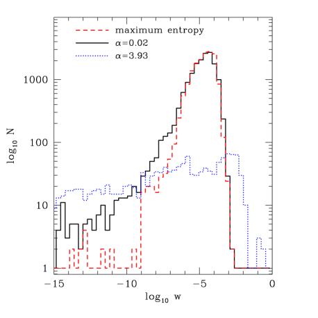
Figure 17: Distribution of orbital weights for three differently regularised models (as indicated in the plot). All models are calculated in the best-fitting mass distribution of GMP5975.

10 Discussion and summary

We have surveyed axisymmetric Schwarzschild models for a sample of 17 Coma early-type galaxies. The models are fitted to measurements of line-of-sight velocity distributions out to $1-4\,r_{\mathrm{eff}}$. Stellar mass-to-light ratios and dark halo parameters are determined for two parameterised halo families with different inner and outer density slopes. The models are regularised towards maximum entropy.

10.1 Luminous and dark matter

In each galaxy, models with dark matter fit better than models without. A constant mass-to-light ratio is significantly ruled out in about half of the sample (eight galaxies where dark matter is detected on at least the 95 percent confidence level). In four galaxies the case for dark matter is weak. The mass distribution in one of these systems (GMP1990) is in fact consistent to follow the light. Five galaxies are intermediate cases where the formal evidence for dark matter is low, although fits with and without dark matter differ systematically in either their radial dispersion profiles or in their outermost LOSVDs. We believe that the low signal for dark matter in these systems is partly due to our very conservative treatment of the error bars.

Our inferences about dark matter are based on the mass decomposition provided by equation (1). In particular, we have assumed that the stellar mass-to-light ratio is constant throughout the galaxy. In this context, GMP1990 is not surrounded by significant amounts of dark matter. However, before finally concluding upon dark matter in our galaxies a detailed comparison to independent estimates of the stellar mass is required (Thomas et al. 2007a, in preparation). For example, GMP1990 has a large mass-to-light ratio $\Upsilon=10.0$ ($R_{C}$-band). If the actual stellar mass can only account for a fraction of it, then our result does not argue against dark matter in this galaxy, but merely implies that dark matter follows closely the light of the system.

Constant mass-to-light ratios have been reported to be consistent with planetary nebulae kinematics in the outskirts of three roundish objects (spherical modelling; Romanowsky et al. 2003). Also some of the round and non-rotating ellipticals of Kronawitter et al. (2000) are consistent with the mass distribution following the light distribution. Many of these latter systems lack of kinematic data beyond $r_{\mathrm{eff}}$, however. In addition to the related uncertainties for the outer dark halo, spherical modelling of round galaxies generally suffers from the ambiguity related to the flattening along the line-of-sight. In this sense, GMP1990 is an interesting case, because its apparent flattening implies a viewing-angle close to $i=90\degr$ and the kinematic data extend relatively far out ($3\,r_{\mathrm{eff}}$).

Best-fit dark matter halos are in 4 out of 17 cases of the NFW-type and in all other cases logarithmic. Differences in the goodness-of-fit based on one or the other halo family are marginal in most cases. Central dark matter densities are at least one to two orders of magnitude lower than the corresponding mass densities in stars. Between 10 and 50 percent of the mass inside the half-light radius $r_{\mathrm{eff}}$ is formally dark in most Coma galaxies. These dark matter fractions are in general agreement with earlier results of dark matter modelling in round, non-rotating ellipticals (Gerhard et al., 2001) as well as with the analysis of cold gas kinematics (Bertola et al., 1993; Oosterloo et al., 2002), hot halo gas (Loewenstein & White, 1999; Fukazawa et al., 2006; Humphrey et al., 2006) and strong lensing studies (Keeton, 2001; Treu & Koopmans, 2004). Cappellari et al. (2006) concluded for similar dark matter fractions in the SAURON-ellipticals (although in their models it is assumed that mass follows light).

The combination of luminous and dark matter results in circular velocity curves of various shapes: some galaxies have outer decreasing $v_{\mathrm{circ}}$ while others show an indication for a dip in $v_{\mathrm{circ}}$ around $\approx 10\,\mathrm{kpc}$ and a subsequent increase of $v_{\mathrm{circ}}$ towards larger radii. We cannot easily quantify the significance of this dip. Its appearance close to the outermost kinematic radius is suspicious to reflect a modelling artifact. However, in contrast to the orbital structure, whose reconstruction becomes uncertain around (and beyond) the last kinematic data point (Krajnović et al., 2005; Thomas et al., 2005), the mass reconstruction in these regions is more robust (Thomas et al., 2005). In addition, the dip does not appear in all galaxies, suggesting that it is related to some observable property of the corresponding objects. In any case, it is interesting to note that similar dips are also indicated in temperature profiles of elliptical galaxy X-ray halos (Fukazawa et al., 2006) and can also been seen in spherical models of some round galaxies (Gerhard et al., 2001). More extended kinematic data sets may in the future allow to better constrain the outer shape of the circular velocity curve.

In rotating systems the circular velocity is fairly constant over the observationally sampled radial region (10 percent fractional variation). Similarly flat circular velocity curves have also been inferred from stellar kinematics of round systems (spherical modelling; Gerhard et al. 2001; Magorrian & Ballantyne 2001) and from strong gravitational lensing (Koopmans et al., 2006).

To the resolution of our orbit models all dark halos are supported by at least one positive definite phase-space distribution function. In case of NFW-halos smooth DFs can be constructed, but for LOG-halos with large core radii even the maximisation of orbital entropy does not yield smooth DFs. It is not obvious whether the corresponding spatial density profiles are stable or not. Further modelling is required to investigate whether phase-space arguments can be used to rule out logarithmic halos in elliptical galaxies.

10.2 Kinematics

With decreasing total mass the influence of rotation on the stellar phase-space distribution increases. In many galaxies rotation arises by an overpopulation of prograde orbits and a simultaneous underpopulation of retrograde orbits. At least one system lacks of the depopulation of retrograde orbits, proving that it is not a general artifact of our modelling approach.

Some galaxies show strong tangential anisotropy along the minor-axis. This derives from low minor-axis $H_{4}$-measurements, because observed $H_{4}$ and modelled orbital anisotropy along the minor-axis turn out to be correlated. Slope and zero-point of this correlation are largely independent of regularisation, but – to some degree – stronger regularisation tightens the relation. Such a relation between an intrinsic quantity on the one hand and an observed one on the other cannot originate from the entropy maximisation alone.

Along the major-axis, a slight tendency of increasing $\beta_{\varphi}$ with increasing $H_{4}$ is noticeable, but with much larger scatter than along the minor-axis. Only one system shows indication of tangential anisotropy ($\beta_{\vartheta}<0$), all other galaxies are isotropic or mildly radially anisotropic ($\beta_{\vartheta}>0$, $\beta_{\varphi}\ga 0$). Radial anisotropy also appears characteristic for spherical models of round galaxies (Kronawitter et al., 2000; Gerhard et al., 2001). A suppression of vertical energy (corresponding to $\beta_{\vartheta}>0$) has recently been reported for SAURON ellipticals (Cappellari et al., 2007). We plan a detailed investigation of the orbital structure of the Coma galaxies for the future.

10.3 Regularisation

Stellar mass-to-light ratios, dark matter fractions and the shape of circular velocity curves turn out to be robust against different choices of the regularisation parameter $\alpha$. The strongest effect $\alpha$ has is on the reconstructed anisotropies: their absolute values tend to increase if the weight on regularisation constraints is lowered. At a fixed radius the dependency of anisotropy on $\alpha$ is mostly monotonic, such that the general quality of a galaxy to be radially or tangentially anisotropic, respectively, is independent of $\alpha$. What changes instead is the actual amount of anisotropy.

10.4 Outlook

Detailed investigations of luminous and dark matter scaling relations, of stellar population properties and their connection to the phase-space distribution of orbits are in preparation.

Appendix A Data fits

Figs. 18 - 34 survey the fits to the photometric and kinematical data for each galaxy (galaxies are arranged in order of decreasing total mass inside $r_{\mathrm{eff}}$).

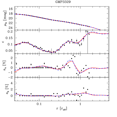
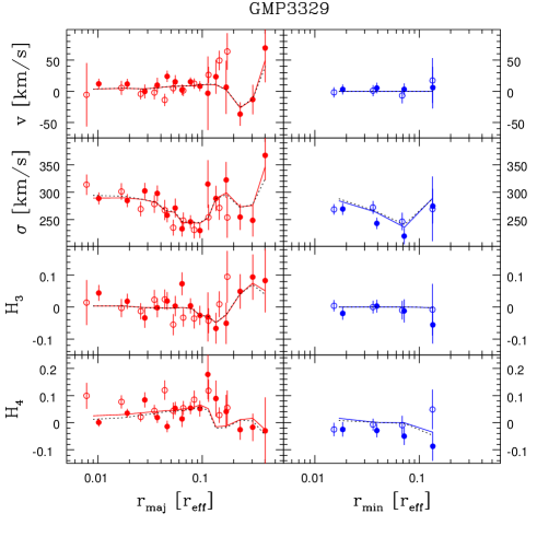
Figure 18: Upper panel: Joint ground-based and HST photometry of GMP3329/NGC 4874. Lines: best-fit deprojection (red) and its edge-on reprojection (blue). Lower panel: stellar kinematics along major (left/red) and minor axis (right/blue); filled and open circles refer to the two sides of the galaxy; dotted: best-fit model without dark matter.

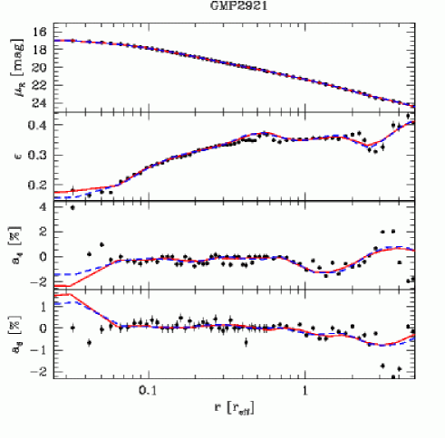
Figure 19: As Fig. 18, but for GMP2921/NGC 4889.

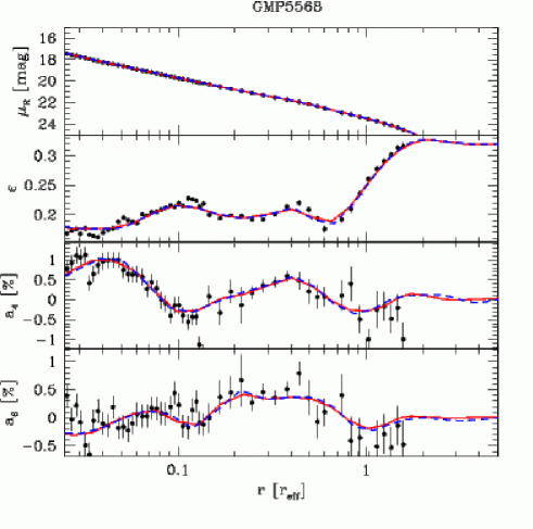
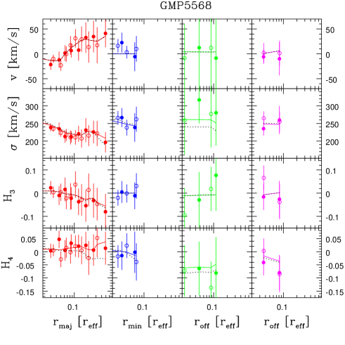
Figure 20: As Fig. 18, but for GMP5568/NGC 4816. Green/third column: offset to major-axis $r_{\mathrm{eff}}/4$; magenta/fourth column: offset to major-axis $r_{\mathrm{eff}}/20$.

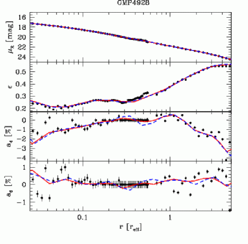
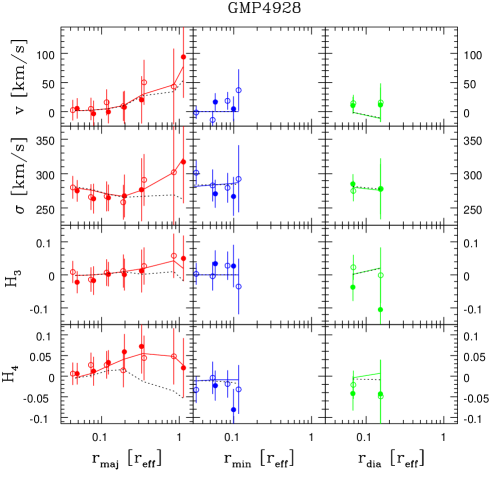
Figure 21: As Fig. 18, but for GMP4928/NGC 4839; green/third column: diagonal axis.

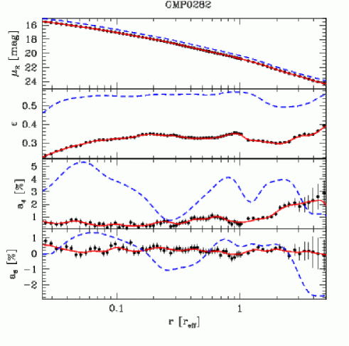
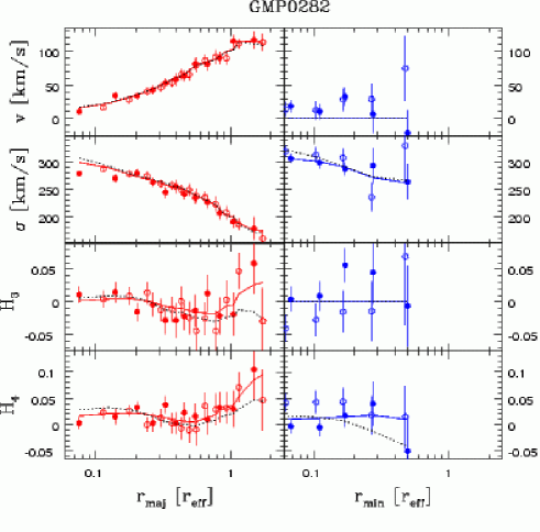
Figure 22: As Fig. 18, but for GMP0282/NGC 4952.

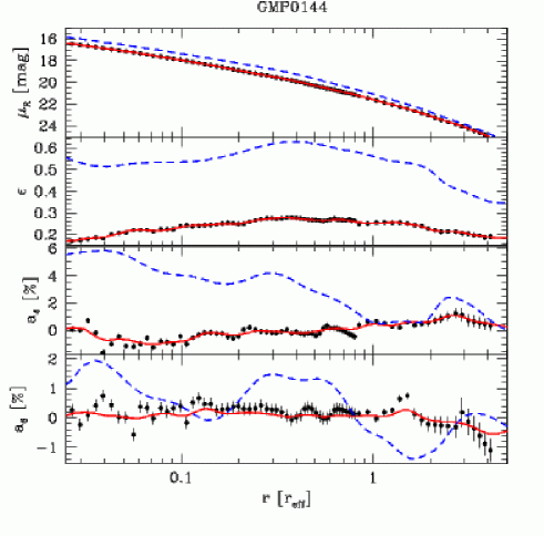
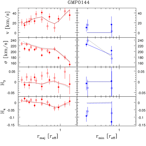
Figure 23: As Fig. 18, but for GMP0144/NGC 4957.

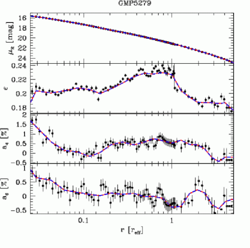
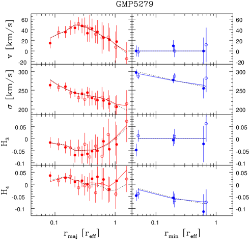
Figure 24: As Fig. 18, but for GMP5279/NGC 4827.

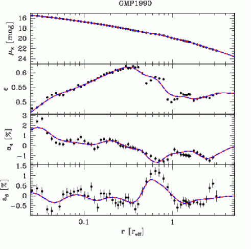
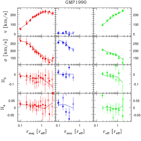
Figure 25: As Fig. 18, but for GMP1990/IC 843; green/third column: offset to major-axis $r_{\mathrm{eff}}/3$.

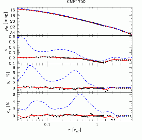
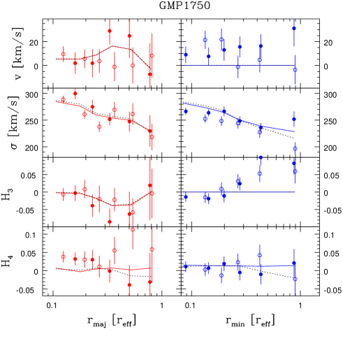
Figure 26: As Fig. 18, but for GMP1750/NGC 4926.

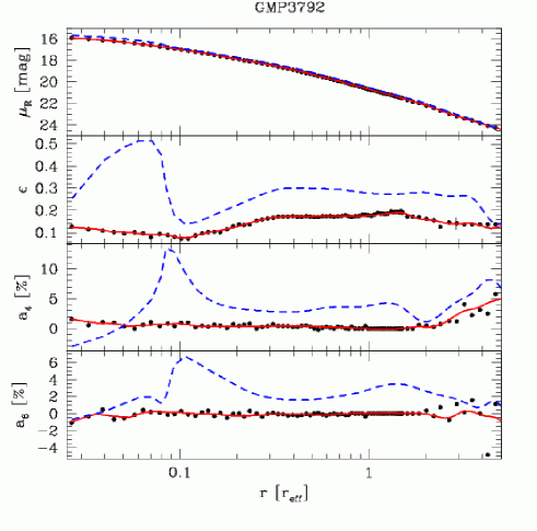
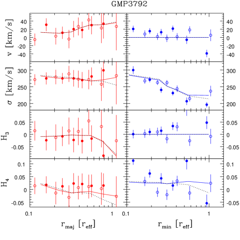
Figure 27: As Fig. 18, but for GMP3792/NGC 4860.

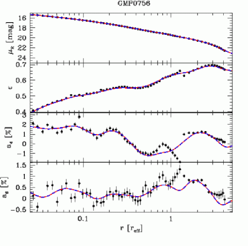
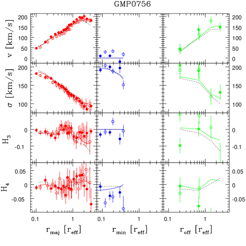
Figure 28: As Fig. 18, but for GMP0756/NGC 4944; green/third column: offset to major-axis $r_{\mathrm{eff}}/2$ (the two outermost $H_{4}<-0.1$ are omitted in the plot).

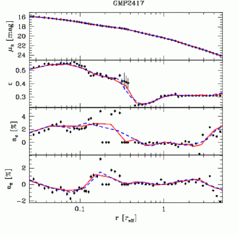
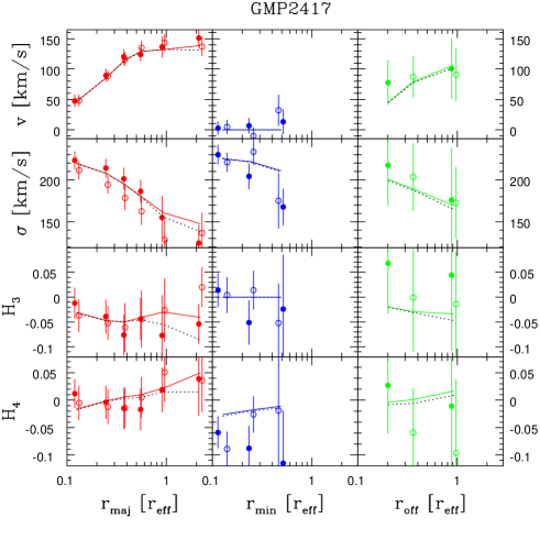
Figure 29: As Fig. 18, but for GMP2417/NGC 4908; green/third column: offset to major-axis $r_{\mathrm{eff}}/2$.

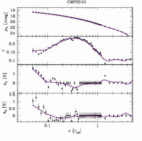
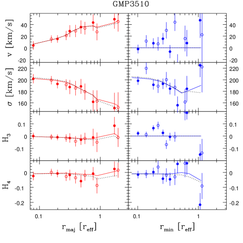
Figure 30: As Fig. 18, but for GMP3510/NGC 4869.

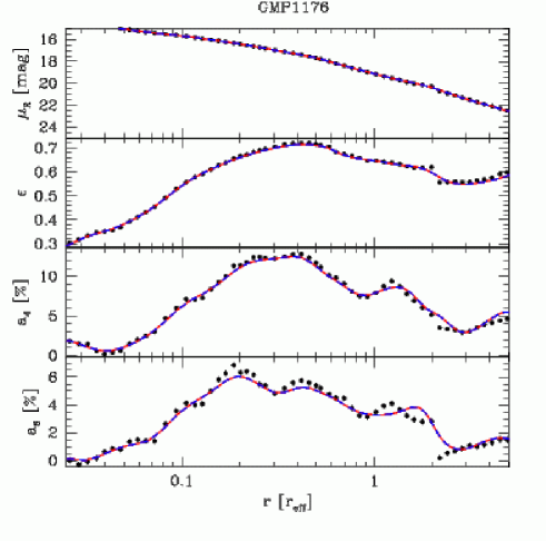
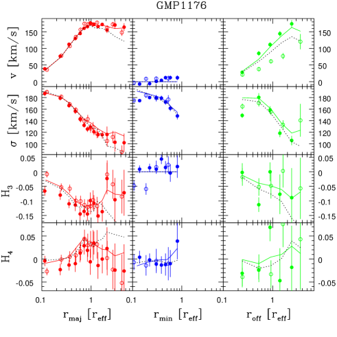
Figure 31: As Fig. 23, but for GMP1176/NGC 4931; green/third column: offset to major-axis $r_{\mathrm{eff}}/3$.

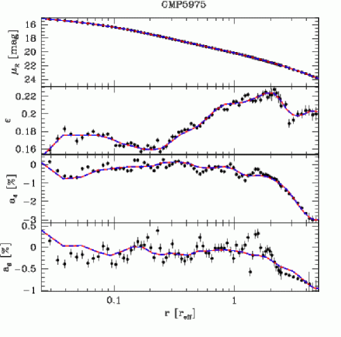
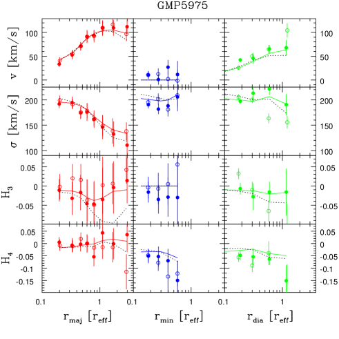
Figure 32: As Fig. 18, but for GMP5975/NGC 4807; green/third column: diagonal axis.

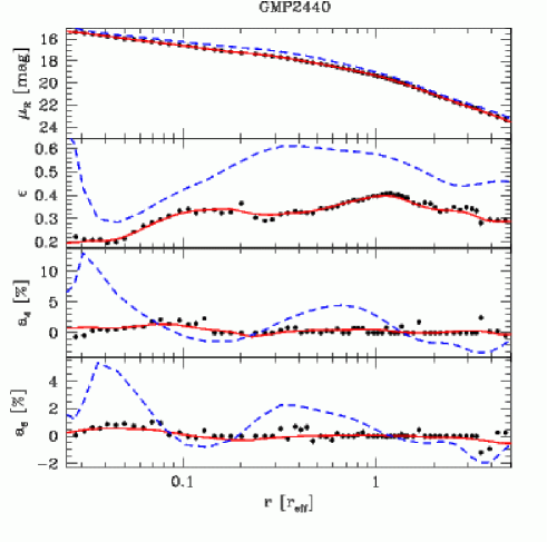
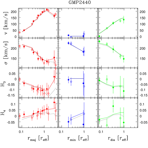
Figure 33: As Fig. 18, but for GMP2440/IC 4045; green/third column: diagonal axis.

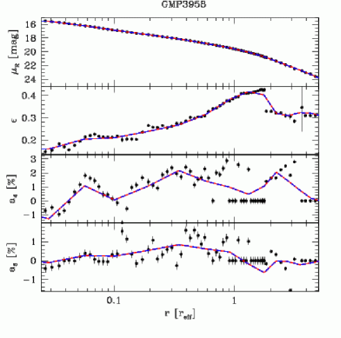
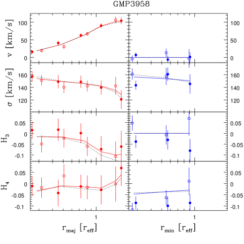
Figure 34: As Fig. 18, but for GMP3958/IC 3947.

References

- Baes, Dejonghe & Buyle (2003) Baes M., Dejonghe H., Buyle P., 2003, A&A, 432, 411
- Bender & Möllenhoff (1987) Bender R., Möllenhoff C., 1987, A&A, 177, 71
- Bertola et al. (1993) Bertola F., Pizzella A., Persic M., Salucci P., 1993, ApJL, 416, 45
- Binney (1981) Binney J., 1981, MNRAS, 196, 455
- Binney & Tremaine (1987) Binney J., Tremaine S., 1987, Galactic Dynamics (Princeton: Princeton University Press)
- Cappellari et al. (2006) Cappellari M. et al., 2006, MNRAS, 366, 1126
- Cappellari et al. (2007) Cappellari M. et al., 2007, MNRAS, in press
- Ciotti & Pellegrini (1992) Ciotti L., Pellegrini S., 1992, MNRAS,255, 561
- Ciotti (1996) Ciotti L., 1996, ApJ, 471, 68
- Ciotti (1999) Ciotti L., 1999, ApJ, 520, 574
- Corsini et al. (2007) Corsini E. M., Wegner G., Saglia R. P., Thomas J., Bender R., Thomas D., submitted to ApJS
- Dubinski (1998) Dubinski J., 1998, ApJ, 502, 141
- Evans (1993) Evans N. W., 1993, MNRAS, 260, 191
- Fukazawa et al. (2006) Fukazawa Y., Botoya-Nonesa J. G., Pu J., Ohto A., Kawano N., 2006, ApJ, 636, 698
- Fukugita, Hogan & Peebles (1998) Fukugita M., Hogan C. J., Peebles P. J. E., 1998, ApJ, 503, 518
- Gebhardt et al. (2000) Gebhardt K. et al., 2000, AJ, 119, 1157
- Gebhardt et al. (2003) Gebhardt K. et al., 2003, ApJ, 583, 92
- Gerhard (1993) Gerhard O. E., 1993, MNRAS, 265, 213
- Gerhard et al. (2001) Gerhard O. E., Kronawitter A., Saglia R. P., Bender R., 2001, AJ, 121, 1936
- Gerhard et al. (2007) Gerhard O. E., Arnaboldi M., Freeman K. C., Okamura S., Kashikawa N., Yasuda N., 2007, A&A, 468, 815
- Godwin, Metcalfe & Peach (1983) Godwin J. G., Metcalfe N., Peach J. V., 1983, MNRAS, 202, 113
- Hernquist (1992) Hernquist L., 1992, ApJ, 409, 548
- Hernquist (1993) Hernquist L., 1993, ApJ, 400, 460
- Hoekstra et al. (2004) Hoekstra H., Yee H. K. C., Gladders M. D., 2004, ApJ, 606, 67
- Humphrey et al. (2006) Humphrey P. J., Buote, D. A., Gastaldello F., Zappacosta L., Bullock J. S., Brighenti F., Mathews W. G., 2006, preprint (astro-ph/0601301)
- Jesseit, Naab & Burkert (2005) Jesseit R., Naab T., Burkert A., 2005, MNRAS, 360, 1185
- Jing & Suto (2000) Jing Y. P., Suto Y., 2000, ApJ, 529, L69
- Jørgensen & Franx (1994) Jørgensen I., Franx M., 1994, ApJ, 433, 553
- Keeton (2001) Keeton C. R., 2001, ApJ, 561, 46
- Kleinheinrich et al. (2006) Kleinheinrich M. et al., 2006, A&A, 455, 441
- Koopmans et al. (2006) Koopmans L. V. E., Treu T., Bolton A. S., Burles S., Moustakas L. A., 2006, ApJ, 649, 599
- Krajnović et al. (2005) Krajnović D., Cappellari M., Emsellem E., McDermid R. M., de Zeeuw P. T., 2005, MNRAS, 357, 1113
- Kronawitter et al. (2000) Kronawitter A., Saglia R. P., Gerhard O. E., Bender R., 2000, A&AS, 144, 53
- Loewenstein & White (1999) Loewenstein M., White R. E., 1999, ApJ 518, 50
- Magorrian (1999) Magorrian J., 1999, MNRAS, 302, 530
- Magorrian & Ballantyne (2001) Magorrian J., Ballantyne D., 2001, MNRAS, 322, 702
- Mandelbaum et al. (2006) Mandelbaum R., Seljak U., Kauffmann G., Hirata C., Brinkmann J., 2006, MNRAS, 368, 715
- Mehlert et al. (1998) Mehlert D., Saglia R. P., Bender R., Wegner G., 1998, A&A, 332, 33
- Mehlert et al. (2000) Mehlert D., Saglia R. P., Bender R., Wegner G., 2000, A&AS, 141, 449
- Naab & Burkert (2003) Naab T., Burkert A., 2003, ApJ, 597, 893
- Navarro, Frenk & White (1996) Navarro J. F., Frenk C. S., White S. D. M., 1996, ApJ, 462, 563
- Oosterloo et al. (2002) Oosterloo T. A., Morganti R., Sadler E. M., Vergani D., Caldwell N., 2002, AJ, 123, 729
- Pierce et al. (2006) Pierce M. et al., 2006, MNRAS, 366, 1253
- Pizzella et al. (1997) Pizzella A. et al., 1997, A&A, 323, 349
- Renzini (2006) Renzini A., 2006, ARA&A, 44, 141
- Richstone & Tremaine (1988) Richstone D. O., Tremaine S., 1988, ApJ, 327, 82
- Rix et al. (1997) Rix H. W., de Zeeuw P. T., Cretton N., van der Marel R. P., Carollo C. M., 1997, ApJ, 488, 702
- Romanowsky et al. (2003) Romanowsky A. J., Douglas N. G., Arnaboldi M., Kuijken K., Merrifield M. R., Napolitano N. R., Capaccioli M., Freeman K. C., 2003, Sci, 301, 1696
- Saglia et al. (2000) Saglia R. P., Kronawitter A., Gerhard O. E., Bender R., 2000, AJ, 119, 153
- Schwarzschild (1979) Schwarzschild M., 1979, ApJ, 232, 236
- Thomas et al. (2004) Thomas J., Saglia R. P., Bender R., Thomas D., Gebhardt K., Magorrian J., Richstone D., 2004, MNRAS, 353, 391
- Thomas et al. (2005) Thomas J., Saglia R. P., Bender R., Thomas D., Gebhardt K., Magorrian J., Corsini E. M., Wegner G., 2005, MNRAS, 360, 1355
- Thomas et al. (2007b) Thomas J., Jesseit R., Naab T., Saglia R. P., Burkert A., Bender R., MNRAS in press
- Tremblay & Merritt (1996) Tremblay B., Merritt D., 1996, AJ, 111, 2243
- Treu & Koopmans (2004) Treu T., Koopmans L. V. E., 2004, ApJ, 611, 739
- van Albada (1982) van Albada T. S., 1982, MNRAS, 201, 939
- van der Marel & Franx (1993) van der Marel R. P., Franx M., 1993, ApJ, 407, 525
- Vincent & Ryden (2005) Vincent R. A., Ryden B. S., 2005, ApJ, 623, 137
- Wechsler et al. (2002) Wechsler R. H., Bullock J. S., Primack J. R., Kravtsov A. V., Dekel A., 2002, ApJ, 568, 52
- Wegner et al. (2002) Wegner G., Corsini E. M., Saglia R. P., Bender R., Merkl D., Thomas D., Thomas J., Mehlert D., 2002, A&A, 395, 753
- Weil & Hernquist (1996) Weil M., Hernquist L., 1996, ApJ, 457, 51