The Gonihedric Ising Model and Glassiness

1 (Pre-)History of the Model

The Gonihedric $3D$ Ising model is a lattice spin model in which planar Peierls boundaries between $+$ and $-$ spins can be created at zero energy cost. Instead of weighting the area of Peierls boundaries as the case for the usual $3D$ Ising model with nearest neighbour interactions, the edges, or “bends” in an interface are weighted, a concept which is related to the intrinsic curvature of the boundaries in the continuum.

The model is a generalised Ising model living on a cubic $3D$ lattice with nearest neighbour, next to nearest-neighbour and plaquette interactions. The ratio between the couplings of these three terms is fixed to a one parameter family which endows the model with unusual properties both in and out of equilibrium. Of particular interest for the discussion here will be that the model manifests all the indications of glassy behaviour without any recourse to quenched disorder, whilst still possessing a crystalline low temperature phase in equilibrium.

In these notes we follow a roughly chronological order by first reviewing the background to the formulation of the model, before moving on to the elucidation of the equilibrium phase diagram by various means and then to the investigation of the non-equilibrium, glassy behaviour of the model. We apologize in advance for our narrow focus on things Gonihedric at the expense of other lattice models with glassy behaviour, since the aim is to concentrate on giving an overview of the Gonihedric Ising model in $3D$.

The model has an unusual genesis since it was originally introduced as a potential discretization of string theory. The Nambu-Goto 1 action (or Hamiltonian in statistical mechanical language) in bosonic string theory is given by the area swept out by the string worldsheet as it moves through spacetime. Directly discretizing euclideanized versions of this action produced ensembles of surfaces, i.e. string worldsheets, which were dominated by collapsed and irregular configurations such as that in Fig.1

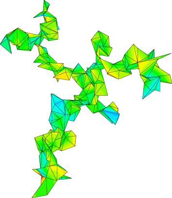
Figure 1: A typical collapsed triangulated surface resulting from a simulation of the Gaussian Hamiltonian in equ.1.

and which were unsuitable for taking any sort of continuum limit 2 . This was presumably a reflection of the well-known tachyonic instability of the bosonic string and therefore not entirely unexpected. The interest was in whether any straightforward modifications of such Hamiltonians did allow a continuum limit, and hence some insight into stable string theories in physical dimensions.

Discretizing the Polyakov 3 form of the string action, which is equivalent to the Nambu-Goto formulation, by triangulating an embedded surface gives the simple Gaussian Hamiltonian

$$H={1\over 2}\sum_{\langle ij\rangle}(\vec{X}_{i}-\vec{X}_{j})^{2}$$ (1)

where the vectors $\vec{X}_{i}$ live on the vertices of the triangulated surface and determine where the vertices sit in the embedding space. The sum $\langle ij\rangle$ is carried out over the edges of the triangulation and in principle one should also sum over different triangulations of the surface as a discretized version of the sum over metrics in the continuum string theory with the Polyakov action. In any case, the observed behaviour of surfaces turns out to be rather similar in ensembles with and without this sum. One possibility for stabilising the surfaces produced by such Hamiltonians is to add an extrinsic curvature term as suggested first in the continuum by Polyakov and Kelinert 4 , which acts to prevent the surfaces collapsing

$$H={1\over 2}\sum_{\langle ij\rangle}(\vec{X}_{i}-\vec{X}_{j})^{2}+\lambda\sum_{\Delta_{i},\Delta_{j}}(1-\vec{n}_{i}\cdot\vec{n}_{j})$$ (2)

where the $\vec{n}_{i},\vec{n}_{j}$ are normals on adjacent triangles $\Delta_{i},\Delta_{j}$. The second term tends to align the normals on adjacent triangles and hence to “stiffen” or flatten out the surface 5 , at least over short length scales.

Figure 2: A typical uncollapsed triangulated surface resulting from a simulation of the Gaussian plus extrinsic curvature Hamiltonian in equ.2 with $\lambda=1.1$.

The issue for Monte Carlo simulations is to determine whether this flattening is also effective on macroscopic length scales.

Another possibility, which also uses a geometrical concept and which has some appealing features from the string theory point of view 6 , is to take an action proportional to the linear size of a surface – a notion first introduced by Steiner 6a . This can be discretized as

$$H={1\over 2}\sum_{\langle ij\rangle}|\vec{X}_{i}-\vec{X}_{j}|\;\theta(\alpha_{ij}),$$ (3)

on triangulated surfaces, where $\theta(\alpha_{ij})=|\pi-\alpha_{ij}|$ where $\alpha_{ij}$ is the dihedral angle between the embedded neighbouring triangles with a common link $\langle ij\rangle$. The $\theta(\alpha_{ij})$ term also acts to flatten out the surfaces 6b . The elements making up these various possible surface Hamiltonians are shown in Fig.3. The origin of the word Gonihedric is a combination of the Greek words gonia for angle (referring to the dihedral angle) and hedra for base or face (referring to the adjacent triangles).

Figure 3: Two adjacent triangles in a triangulation of a surface with a common edge $\langle ij\rangle$, showing the normals $\vec{n}$, the co-ordinates of the endpoints $\vec{X}_{i,j}$ and the dihedral angle $\alpha_{ij}$

Savvidy and Wegner posed the question of how to translate the essential features of such a Hamiltonian to a surface composed of plaquettes on a cubic (or hypercubic) lattice 7 . This was motivated by the observation that it was possible to rewrite the Hamiltonian for an ensemble of such surfaces by using the geometrical spin cluster boundaries of a suitable generalised Ising model with nearest neighbour, next to nearest-neighbour and plaquette interactions to define the surfaces and their appropriate energies. It is generally much easier to simulate an Ising spin model than a gas of surfaces so one might expect some advantages, both numerical and analytical, from such a reformulation of the system.

On a fixed cubic lattice all the edge lengths $|\vec{X}_{i}-\vec{X}_{j}|$ will be identical, so the statistical weight of a surface configuration will be entirely determined by the $\theta(\alpha_{ij})=|\pi-\alpha_{ij}|$ factors, where the $\alpha_{ij}$ are restricted to multiples of $\pi/2$ radians. In other words, the statistical weight of a plaquette surface configuration will be determined entirely by the number of bends and self-intersections it contains. There is no (bare) weight for the area of a plaquette in the surfaces in contrast to the usual $3D$ Ising model with only nearest neighbour interactions.

The generalised Ising models which are used in the construction are of the form

$$H=J_{1}\sum_{\langle ij\rangle}\sigma_{i}\sigma_{j}+J_{2}\sum_{\langle\langle i,j\rangle\rangle}\sigma_{i}\sigma_{j}+J_{3}\sum_{[i,j,k,l]}\sigma_{i}\sigma_{j}\sigma_{k}\sigma_{l}.$$ (4)

where the Hamiltonian contains nearest neighbour ($\langle i,j\rangle$), next to nearest neighbour ($\langle\langle i,j\rangle\rangle$) and round a plaquette ($[i,j,k,l]$) terms. The couplings in such models can be related to the energy cost for a plaquettes in the Peierls interface $\beta_{A}$, a right-angled bend between two such adjacent plaquettes, $\beta_{C}$, and the energy cost, $\beta_{I}$, for the intersection of four plaquettes having a link in common

$$\beta_{A} = 2J_{1}+8J_{2}$$

$$\beta_{C} = 2J_{3}-2J_{2}$$

$$\beta_{I} = -4J_{2}-4J_{3}\;.$$ (5)

General cases of such Hamiltonians and their equivalent surface formulations had been studied in some detail by Cappi et.al. and found to have a very rich phase structure for generic choices of the couplings 9a , including homogeneous, lamellar, disordered and bicontinuous phases. The Gonihedric model constitutes a particular one-parameter slice in this space of Hamiltonians:

$$H=-2\kappa\sum_{\langle ij\rangle}\sigma_{i}\sigma_{j}+\frac{\kappa}{2}\sum_{\langle\langle i,j\rangle\rangle}\sigma_{i}\sigma_{j}-\frac{1-\kappa}{2}\sum_{[i,j,k,l]}\sigma_{i}\sigma_{j}\sigma_{k}\sigma_{l}.$$ (6)

and for such a ratio of couplings $\beta_{A}=0$, which is the desired zero weight for plaquette area suggested by translating the Hamitonian of equ.(3). The energy of the spin cluster boundaries for this Gonihedric model on a cubic lattice is simply given by

$$E=n_{2}+4\kappa n_{4},$$ (7)

where $n_{2}$ is the number of links where two plaquettes on a spin cluster boundary meet at a right angle, $n_{4}$ is the number of links where four plaquettes meet at right angles, and $\kappa$ is a free parameter which determines the relative weight of a self-intersection of the surface.

The particular ratio of couplings in equ.(6) also introduces a novel semi-global symmetry into the Hamiltonian, as we discuss in the next section. This is related to a zero-temperature high degeneracy point where it is possible to flip non-intersecting planes of spins at zero energy cost. This symmetry is further enhanced at $\kappa=0$ where the action becomes a purely plaquette term

$$H={\bf-}\frac{1}{2}\sum_{[i,j,k,l]}\sigma_{i}\sigma_{j}\sigma_{k}\sigma_{l}.$$ (8)

and any plane of spins, even intersecting ones, may be flipped at zero energy cost at $T=0$, which suggests a highly degenerate ground state for the $\kappa=0$ Gonihedric model. Series expansions and cluster variational calculations, described below, show that the degeneracy of the Hamiltonian is broken in the free energy for $\kappa\neq 0$, indicating a ferromagnetic low temperature phase in this case, but the nature of the order in the low temperature phase for $\kappa=0$ remains rather mysterious.

2 Equilibrium Behaviour, by various means

In what follows we use the standard definitions of quantities such as the magnetisation

$$M={1\over L^{3}}\sum_{i}\sigma_{i}$$ (9)

and the Binder cumulant

$$U=1-{\langle M^{4}\rangle\over 3\langle M^{2}\rangle^{2}},$$ (10)

in discussing critical properties, where the $\langle\rangle$ brackets denote thermal averages.

The energy $\langle E\rangle$ is just given by the average of the Hamiltonian, the specific heat $C$ by the variance of the energy and the susceptibility $\chi$ by the variance of the magnetisation. The scaling exponents are then defined by the singular properties of these quantities at the critical point(s) of the model

$$C=B+C_{0}t^{-\alpha},\;M=M_{0}t^{\beta},\;\chi=\chi_{0}t^{-\gamma},\;\xi=\xi_{0}t^{-\nu}$$ (11)

where $t=|(T-T_{c})/T_{c}|$ is the reduced temperature, $\xi$ is the correlation length and $\nu$ is the correlation length exponent, giving the divergence of the correlation length at criticality.

These can also be recast as finite-size scaling relations

$$C=B^{\prime}+C_{0}^{\prime}L^{\alpha\over\nu},\;M=M_{0}^{\prime}L^{-\beta\over\nu},\;\chi=\chi_{0}^{\prime}L^{\gamma\over\nu}$$ (12)

for lattices of linear extent $L$, which is more convenient when $T_{c}$ is not known exactly, which is usually the case.

Various methods have been used to investigate the phase diagram of the Gonihedric model, ranging from generalised mean field techniques, through cluster variational calculations to Monte Carlo simulations. The gross phase structure of the Gonihedric model was apparent even in the earliest Monte Carlo work 10 , and is shown schematically in Fig.4. For $\kappa=0$ and small values of $\kappa$ there is a first order transition 11 , signified by a jump in the energy, $E$, at the transition point and first order (volume) scaling in the specific heat.

As $\kappa$ was increased the transition softened to second order, but Monte Carlo simulations and other approaches have struggled to produce a consistent set of critical exponents. The first direct Monte-Carlo simulations 10 , for instance, found $\nu=1.2(1),\gamma=1.60(2),\beta=0.12(1)$ when $\kappa=1$, but later work using the scaling of the surface tension of a spin interface 12 obtained $\nu=0.44(2)$ and $\gamma/\nu=2.1(1)$.

Figure 4: The phase transition line as $\kappa$ is varied.

Other approaches also gave results at variance with these: a low temperature expansion by Pietig and Wegner found $\alpha=0.62(3),\beta=0.040(2)$ and $\gamma=1.7(2)$ at $\kappa=1$ 13 ; whilst Cirillo et.al. 14 found $\beta=0.062(3)$ and $\gamma=1.41(2)$ using a combination of the cluster variational method and Padé approximants (“CVPAM”) 15 .

These cluster variational calculations, ground state enumerations and mean field calculations all use a similar starting point – the decomposition of the lattice into elementary cubes and we now discuss these methods in some detail since they are useful in sketching out the phase structure. Indeed, the cluster variational method, allied with Padé approximant techniques has succeeded in providing a very plausible picture of the Gonihedric phase diagram by looking at an extended two-parameter Hamiltonian.

One of the elementary cubes from the $3D$ cubic lattice is shown in Fig.5. The full lattice Hamiltonian may be written as a sum over individual cube Hamiltonians

$$h_{c}=\frac{\kappa}{2}\sum_{\langle i,j\rangle}\sigma_{i}\sigma_{j}-\frac{\kappa}{4}\sum_{\langle\langle i,j\rangle\rangle}\sigma_{i}\sigma_{j}+\frac{1-\kappa}{4}\sum_{[i,j,k,l]}\sigma_{i}\sigma_{j}\sigma_{k}\sigma_{l}\;$$ (13)

which differs from the full Hamiltonian by the symmetry factors in front of each term. If the lattice can be tiled by a cube configuration minimising the individual $h_{c}$ then the ground state energy density is $E_{0}=min\;h_{c}$.

Figure 5: The ground-state and mean field analyses of the Gonihedric model require working with elementary cubes rather than single sites to capture the various possible spin configurations.

We list some of the inequivalent spin configurations on a single cube and their multiplicities in Table.1.

Table 1: Elementary cube ground state energies

State	Top	Bottom	Energy	Multiplicity
$\psi_{0}$	+ +	+ +	$-3/2-3\kappa/2$	2
	+ +	+ +
$\psi_{\bar{0}}$	- +	+ -	$-3/2+21\kappa/2$	2
	+ -	- +
$\psi_{6}$	- -	+ +	$-3/2-3\kappa/2$	6
	- -	+ +
$\psi_{\bar{6}}$	+ +	- -	$-3/2+5\kappa/2$	6
	- -	+ +

In the list of spins the first column represents one face of the cube and the second the other and the notation $\psi_{0},...$ is borrowed from 9a The antiferromagnetic image of a configuration is obtained by flipping the three nearest neighbours and the spin at the other end of the cube diagonal from a given spin and is denoted by an overbar.

With the Gonihedric values of the couplings there is a freedom to flip spin planes in the ground state as $\psi_{0}$, which would represent a ferromagnetic state when used to tile the lattice, and $\psi_{6}$ which would represent flipped spin layers, have the same energy for any value of $\kappa$. The degeneracy increase when $\kappa=0$, the club of states of energy $-3/2$ is now composed of $\psi_{0},\psi_{\bar{0}},\psi_{6},\psi_{\bar{6}}$.

This degeneracy means that the definition of an order parameter for the low-temperature phase is a moot point. The standard magnetisation $M$ will not serve at zero temperature as is clear from consideration of the ground state energies above, since the freedom to flip spin planes means that it is identically zero. As we have noted, it appears that this symmetry is broken for $\kappa\neq 0$ at non-zero temperature, but in Monte Carlo simulations the magnetisation is still indistinguishable from zero, presumably because of the difficulty of removing such flipped planes within the timespan of the simulation. Even staggered magnetizations do not suffice as order parameters as the interlayer spacing between the flipped planes of spins can be arbitrary.

One possibility on a finite lattice is to force the model into the ferromagnetic phase with a suitable choice of boundary conditions such as fixed boundary conditions. Although this allows the use of a standard magnetic order parameter, it does some violence to both the scaling properties and the ground state structure structure itself. The corrections to first-order scaling, for example, are much stronger with fixed boundary conditions than with the more familiar periodic boundary conditions,

Table 2: Scaling laws for Periodic versus Fixed Boundary Conditions for the critical temperature, maxima of the specific heat and susceptibility and minimum of the Binder cumulant. In all cases a d-dimensional cubic lattice of length $L$ is considered.

	P.B.C.	F.B.C.
$\beta_{c}^{peaks}(L)=$	$\beta_{c}(\infty)+\frac{\theta_{1}}{L^{d}}+O(\frac{1}{L^{2d}})$	$\beta_{c}(\infty)+\frac{a_{1}}{L}+O(\frac{1}{L^{2}})$
$C_{max}(L)=$	$\gamma_{0}+\gamma_{2}L^{d}+O(\frac{1}{L^{d}})$	$c_{0}+c_{2}L^{d}+O(L^{d-1})$
$\chi_{max}(L)=$	$\delta_{0}+\delta_{2}L^{d}+O(\frac{1}{L^{d}})$	$e_{0}+e_{2}L^{d}+O(L^{d-1})$
$U_{min}(L)=$	$\Phi_{0}+\frac{\Phi_{1}}{L^{d}}+O(\frac{1}{L^{2d}})$	$B_{0}+\frac{B_{1}}{L}+O(\frac{1}{L^{2}})$

although simulations of the $\kappa=0$ model with fixed boundary conditions have given good agreement with this scaling 16 .

The approach taken to enumerating the ground states by splitting the lattice into elementary cubes can also be applied to mean field theory for the model and to extensions of mean field theory such as the cluster variational method. In the mean field approximation the spins are replaced by the average site magnetizations and an entropy term introduced to give the free energy. In the Gonihedric model the total mean field free energy may be written as the sum of elementary cube free energies $\phi(m_{C})$

$$\phi{(m_{C})} = -\frac{\kappa}{2}\sum_{\langle i,j\rangle\subset C}m_{i}m_{j}+\frac{\kappa}{4}\sum_{\langle\langle i,j\rangle\rangle\subset C}m_{i}m_{j}-\frac{1-\kappa}{4}\sum_{[i,j,k,l]\subset C}m_{i}m_{j}m_{k}m_{l}$$ (14)

$$+ \frac{1}{16}\sum_{i\subset C}[(1+m_{i})ln(1+m_{i})+(1-m_{i})ln(1-m_{i})]$$

where $m_{C}$ is the set of the eight magnetizations of the elementary cube. This in turn gives a set of eight mean-field equations

$$\frac{\partial\phi(m_{C})}{\partial m_{i}}_{(i=1{\ldots}8)}=0$$ (15)

(one for each corner of the cube) rather than the familiar single equation for the standard nearest neighbour Ising action.

If we solve these equations iteratively we arrive at zeroes for a paramagnetic phase or various combinations of $\pm 1$ for the magnetised phases on the eight cube vertices, and the mean field ground state is then given by gluing together the elementary cubes consistently to tile the complete lattice, in the manner of the ground state discussion. Carrying out this program gives a rather simple mean field phase diagram for the Gonihedric model with action equ.(6), with a single transition from a paramagnetic phase to a degenerate “layered” phase that is pushed down to $\beta=0$ at large $\kappa$. The low temperature phase is generically of the $\psi_{0,6}$ type, apart from $\kappa=0$ where we see a $\psi_{\bar{0},\bar{6}}$ phase that is degenerate with these. A more sophisticated treatment using the cluster variational method, described below, suggests that the layered phase has a slightly higher free energy than the ferromagnetic phase so the low temperature phase is in fact the ferromagnetic one when the model is in the regime with a continuous transition.

The cluster variation method, or CVM for short, is based on a truncation of the cluster (cumulant) expansion of the free energy density functional on which the variational formulation of statistical mechanics is based 16a . Unlike mean field theory it generally locates rather accurately the boundaries between different phases in complex phase diagrams and, using the recently proposed cluster variation–Padè approximant method one can extract non-classical, precise estimates of the critical exponents.

For the Gonihedric model, it is again possible to use the cube approximation of the CVM, in which the maximal clusters are the elementary cubic cells of our simple cubic lattice; for this approximation the free energy density functional has the form

$$\phi[\rho_{8}] = {\rm Tr}(\rho_{8}H_{8})+\frac{1}{\beta}\Bigg{[}{\rm Tr}{\cal L}(\rho_{8})-\frac{1}{2}\sum_{\rm plaquettes}{\rm Tr}{\cal L}(\rho_{4,{\rm plaquette}})$$ (16)

$$+\frac{1}{4}\sum_{\rm edges}{\rm Tr}{\cal L}(\rho_{2,{\rm edge}})-\frac{1}{8}\sum_{\rm sites}{\rm Tr}{\cal L}(\rho_{1,{\rm site}})\Bigg{]},$$

where $H_{8}$ is the contribution of a single cube to the Hamiltonian, ${\cal L}(x)=x\ln x$, $\rho_{\alpha}$ with $\alpha=8$ (4, 2, 1) denotes the cube (respectively plaquette, edge, site) density matrix, and the sums in the entropy part are over all plaquettes (edges, sites) of a single cube.

Since the cluster variation method can be viewed as a generalised mean field theory, it is clear that it can give only classical predictions for the critical exponents. In order to overcome this difficulty, one can use the cluster variation–Padè approximant method (CVPAM), which has proven to be a quite accurate technique for extracting exponents. The basic idea of the CVPAM is that, since the CVM gives for Ising-like models very accurate results far enough from the critical point, one can try to extrapolate these results in order to study the critical behaviour. In order to determine the critical exponent of an order parameter $M$, for example, one calculates $M(\beta)$ with the CVM up to a temperature at which the error can be estimated to be very small (typically of order $10^{-5}$), and then constructs, by a simple interpolation, Padè approximants for the logarithmic derivative of $M(\beta)$: the pole and the corresponding residue of each Padè approximant are then estimates for the critical temperature and for the critical exponent respectively 15 .

The CVPAM calculations give a phase diagram whose topology agrees with Monte Carlo simulations 14 . The value for the magnetic exponent is found to be $\beta=0.062\pm 0.003$. Another important observation from the CVPAM calculations is that at finite temperatures there is a violation of the flip symmetry of the Gonihedric Hamiltonian when $\kappa\neq 0$, so that in the ordered region of the model the ferromagnetic phase is always stable with respect to the lamellar phase.

Applying CVPAM methods to a slight extension to the Gonihedric Hamiltonian gives useful insight into the nature of the phase diagram 17 . The Hamiltonian is modified to

$$H=-\sum_{\langle ij\rangle}\sigma_{i}\sigma_{j}-j\sum_{\langle\langle i,j\rangle\rangle}\sigma_{i}\sigma_{j}-{1-\kappa\over 4\kappa}\sum_{[i,j,k,l]}\sigma_{i}\sigma_{j}\sigma_{k}\sigma_{l}.$$ (17)

with a second parameter $j$ which reduces to the Gonihedric model, with suitably rescaled couplings, when $j=-0.25$. The CVPAM calculations (and independent transfer matrix calculations 18 ) for this modified Hamiltonian give a phase diagram whose $\kappa=1$ slice is shown in Fig.6.

Figure 6: A $\kappa=1$ slice of the two-parameter Hamiltonian phase diagram.

The structure of this phase diagram gives some strong hints as to why the critical exponent measurements in Monte Carlo simulations have been so inconsistent. The dotted line in Fig.6 is the usual $3D$ ferromagnetic Ising transition, along which the standard $3D$ Ising critical exponents such as $\nu=0.6294$ would be observed. The line separating the lamellar and ferromagnetic phases appears to be bent slightly to the left according to both CVPAM and transfer matrix calculations. The observed Gonihedric model transition will thus be strongly influenced by crossover effects close to the endpoint of the standard Ising line which which is near, but not exactly at, $j=-0.25$.

In such a case we would expect the correlation length to diverge as

$$\xi\sim N^{\pm}t^{-\nu}$$ (18)

where the new feature is the critical amplitude, which is given by

$$N^{\pm}\propto\Delta^{(-\dot{\nu}+\nu)/\phi}$$ (19)

with $\dot{\nu}$ and $\nu$ being the tricritical and $3D$ Ising values for the correlation length exponent respectively, and $\Delta=j+0.25$. While CVPAM and transfer matrix calculations 17 ; 18 are both in agreement with this general picture the values obtained for the tricritical exponents and crossover exponent do not agree, the transfer matrix calculations finding $\dot{\nu}=0.45(15)$ and $\phi=0.6(2)$, whereas the CVPAM calculation finds $\phi=1.1(1)$.

In summary, while the general features of the Gonihedric model equilibrium phase diagram are understood both for $\kappa=0$ and $\kappa\neq 0$ and a plausible tricritical/crossover scaling scenario has been advanced to describe the observed values of the critical exponents, these have still not been determined with any great degree of certainty. It is also difficult to define a suitable magnetic order parameter for the low-temperature phase as the flip symmetry of the Hamiltonian means the standard magnetisation will be zero in the ground state. Although both low temperature expansions and CVPAM calculations of the free energy strongly suggest that this symmetry is broken for non-zero $\kappa$ at finite temperature, the standard magnetisation is still measured to be zero in the low temperature phase in Monte-Carlo simulations for $\kappa\neq 0$. The flip symmetry appears to be unbroken for the $\kappa=0$ (pure plaquette) case, so the low temperature phase for this is highly degenerate.

A further difficulty which has been observed in attempting to extract critical exponents via Monte Carlo simulations is the very long autocorrelation times which the model exhibits, as was first remarked in 18a . These have the effect of smearing out the observed critical singularities and rendering the extraction of critical exponents problematic. With this in mind, we now turn to the non-equilibrium properties.

3 Non-Equilibrium Behaviour, mostly by Monte Carlo simulations

On heuristic grounds we would expect slow dynamics in the Gonihedric model since the destruction of a spin droplet will require an activation energy because of the weighting of any new edges in the Gonihedric Hamiltonian.

Figure 7: Destroying a cubic excitation, by “nibbling” away the edges has an activation energy in the Gonihedric model.

Indeed, when $\kappa=1$ the plaquette term drops out and one is left with

$$H=-2\sum_{\langle ij\rangle}\sigma_{i}\sigma_{j}+\frac{1}{2}\sum_{\langle\langle i,j\rangle\rangle}\sigma_{i}\sigma_{j}\,.$$ (20)

which represents a particular case of a class of models with competing nearest neighbour and next-nearest neighbour interactions formulated by Shore and Sethna specifically to investigate slow dynamics 19 . We will denote such models with generic coupling ratios Shore and Sethna models below. The Gonihedric Hamiltonian with $\kappa=1$ displays some differences in its dynamics compared with the generic case.

Hand in hand with such slow dynamics and energy barriers we would also expect to see metastability in the model and this is backed up by both CVPAM calculations and direct integration in Monte Carlo simulations to obtain the free energy. For $\kappa=0$ the CVPAM calculations of the free energy show a region of metastability both above and below the first order transition point at $\beta=T^{-1}\sim 0.55$ 14 .

Figure 8: The free energy from a CVPAM calculation when $\kappa=0$. The solid line is the low temperature phase and the dashed dotted line the high temperature paramagnetic phase.

To calculate the free energy of the model in a Monte Carlo simulation 20 we used the following equations:

$$\phi_{{\rm lowT}} = E-T\int_{0}^{T}\frac{C}{T}\;dT,$$

$$\phi_{{\rm highT}} = -Ts(\infty)+T\int_{0}^{1/T}E\;d(\frac{1}{T}).$$ (21)

In the above equation $C$ and $E$ denote the specific heat and internal energy, respectively (measured using the standard formulae in the Monte Carlo simulation), and $s(\infty)=\ln(2)$ is the entropy per site at infinite temperature.

Figure 9: The free energy from a Monte Carlo simulation when $\kappa=0$. The transition point and the region of metastability are both in excellent agreement with the CVPAM calculation of Fig.8.

We also find, see Fig.10 and as advertised earlier, that the lamellar low temperature phase has a higher free energy than the ferromagnetic phase when $\kappa=1$

Figure 10: The free energy from a CVPAM calculation when $\kappa=1$. The solid line is the ferromagnetic phase, the dashed dotted line the high temperature paramagnetic phase and the dashed line the lamellar phase

indicating that the true low temperature phase is ferromagnetic in this case, although this does not appear to be realised within the timescale of Monte Carlo simulations carried out so far.

Qualitative numerical experiments provide plenty of evidence for interesting dynamical behaviour in the model, particularly with respect to quenches 20 . In the $\kappa=0$ case to study the evolution of a random configuration quenched to low temperature, one can measure the energy excess $\delta E(t)=E(t)-E_{0}$ over the ground state energy $E_{0}$. One expects that the inverse of this quantity sets the characteristic length scale of the system $l(t)$, which roughly corresponds to the average size of domains. There is convincing evidence that the generic behaviour in many systems with nonconservative dynamics and scalar order parameter (i.e., conditions which are satisfied here) $l(t)$ increases asymptotically in time as $l(t)\sim t^{n}$ and $n=1/2$. However, in some systems $l(t)$ is known to increase much more slowly in time, even logarithmically $l(t)\sim{\rm log}(t)$. These rather exceptional systems include some random (at the level of the Hamiltonian) systems, and also the Shore and Sethna models at sufficiently low temperatures. It is the energy barriers developing in these systems during the coarsening which cause such a slow increase of $l(t)$, so the Gonihedric model would also be a good candidate for such behaviour.

The log-log plot of $1/\delta E(t)$ as a function of time for the Gonihedric model with $\kappa=0$ is shown in Fig.11 The presented results are obtained for $L=40$ but very similar behaviour was observed for $L=30$.

Figure 11: The excess energy over the groundstate vs time during a quench to various temperatures. The dotted line represents generic coarsening behaviour with an exponent of $1/2$.

From Fig.11 it is clear that for $T=0.75$ and $1.4$ the asymptotic slopes of the curves are much smaller than 1/2 and there is a tendency for these curves to bend downwards. Taking into account the absence of models with $n$ considerably smaller than 1/2 and the existence of energy barriers in the Gonihedric model of basically the same nature as in the Shore and Sethna model, suggests that for the examined temperatures the characteristic length asymptotically increases logarithmically in time. It would appear that such a slow increase of $l(t)$ takes place even for $T=1.65$ and $1.7$, but the behaviour of $l(t)$ for these temperatures is obscured by the metastability effects, since before collapsing into the glassy phase the system remains in the liquid state for some time.

The difference between the Gonihedric model and the Shore and Sethna model becomes clear when we approach the lower boundary of the metastable region which we roughly estimate to lie at $T=T_{{\rm l}}\sim 1.7$ by increasing the temperature. In the Shore and Sethna model for temperatures below the critical point but above a corner-rounding transition thermal fluctuations roughen corners of domains and energy barriers are no longer relevant. Consequently, the standard coarsening dynamics with $n=1/2$ is restored and the system rapidly evolves toward the low-temperature phase. On the contrary, in the Gonihedric model for $1.7<T<1.95$ a random quench does not even evolve toward the low-temperature phase but remains disordered.

The region of metastability can also be investigated through measuring various characteristic times by imposing different initial and boundary conditions and monitoring the evolution toward a final state. To check the decay time associated with the stability of the high temperature “liquid” phase ($\tau_{{\rm liq}}$), a random initial configuration can be used and then simulated at lower temperature until the energy reaches a sufficiently small value. To estimate $\tau_{{\rm liq}}$ around 100 independent runs were necessary. The results for $T=1.75$ are shown in Fig.12 and they suggest that the escape time increases at least exponentially with the system size, which is at first sight surprising for a model with finite range interactions.

A later order of magnitude calculation 21 for the size of a critical droplet (one that would grow and eventually take over the whole system with the stable phase) in the Gonihedric model by Swift et.al. showed that the results discussed here were for system sizes comparable or smaller than such a droplet, so the system size itself was setting the scale of energy barriers, leading to the observed exponential growth in lifetimes. The energy barrier $\Delta$ to forming a droplet of size $R$ would be

$$\Delta=A\sigma R^{d-1}-B\delta fR^{d}$$ (22)

in $d$ dimensions, where $\sigma$ is the surface tension between stable and metastable phases, $\delta f$ is the bulk free energy difference between the two phases and $A$ and $B$ are determined by the geometry of the droplet. Maximising $\Delta$ gives the critical radius $R^{*}$

$$R^{*}={A(d-1)\sigma\over B\delta fd}.$$ (23)

At low $T$ in $3D$ this gives a timescale for the nucleation of such a critical droplet of the form

$$\tau\sim\exp(4A^{3}\sigma^{3}/27B^{2}\delta f^{2}T)$$ (24)

and inserting plausible estimates for $\sigma$ and $\delta f$ in the $\kappa=0$ Gonihedric model gives $R^{*}=25$ for cubic droplets and $\tau\sim 10^{47}$ Monte Carlo steps. F

Figure 12: The size dependence of the logarithm of the escape times $\tau_{{\rm liq}}$ ($\Box$) and $\tau_{+-}$ (+). Calculation of $\tau_{{\rm liq}}$ and $\tau_{+-}$ was done for $T=1.75$ and $T=1.8$, respectively.

To check the stability of the low temperature “crystal” phase, one should measure the time ($\tau_{+}$) needed for the crystal to be transformed into the liquid. It would be particularly interesting to examine the size dependence of $\tau_{+}$ for $1.8<T<1.95$, i.e., for temperatures where the crystal is metastable. It was found, however, that this quantity increases very rapidly with the system size and in this temperature range it is virtually impossible to increase the system size beyond $L=6$. The stability of this phase might be also inferred from measurements of the time ($\tau_{+-}$) needed to shrink a cubic excitation of size $L$. This technique parallels that which has already been applied to the Shore and Sethna model: the initial configuration has “up ” spins at the boundary of the cube of size $L+2$ (which are kept fixed) and “down ” spins inside this cube. Simulations are performed until the magnetisation of the interior of the cube decays to zero and the time needed for such a run is recorded. To calculate $\tau_{+-}$ at a given temperature 100 independent runs were again made. The results for $T=1.8$ suggest that $\tau_{+-}$ increases approximately exponentially with $L$, whereas above the corner-rounding transition in the Shore and Sethna model one expects $\tau_{+-}\sim L^{2}$, in which case the data in Fig.12 would bend noticeably downwards.

Other analogous numerical experiments may be carried out for non-zero $\kappa$ and the tentative picture which emerges 22 is shown in Fig.13.

Figure 13: The phaselines for the Shore-Sethna model (a), the Gonihedric model with a continuous transition (b) and the Gonihedric model with a first order transition (in particular $\kappa=0$) (c).

The salient features are that generic Shore Sethna models with competing nearest neighbour and next nearest neighbour interactions have logarithmically slow low temperature dynamics, with a transition to standard $t^{1/2}$ coarsening behaviour above a corner rounding transition at $T_{cr}$. For the Gonihedric model with a continuous transition (e.g. $\kappa=1$) simulations suggest that this corner rounding transition is pushed close to (or may even be at) the equilibrium critical temperature $T_{c}$. The $\kappa=0$ Gonihedric model displays rather different properties. In this case there is a region of strong metastability on either side of a first order equilibrium transition at $T_{c}$. We tentatively identify the lower boundary of the region of metastability with a glass transition temperature $T_{g}$. We now discuss why it is tempting to do so.

Glassy effects in simulations are usually discerned by looking at appropriate two-time quantities such as the spin-spin autocorrelation

$$C(t,t_{w})=\langle\frac{1}{N}\sum_{i}\sigma_{i}(t_{w})\sigma_{i}(t+t_{w})\rangle$$ (25)

where $N=L^{3}$ and $t_{w}$ is a waiting time before measurements are commenced. Both normal coarsening and glassy dynamics are expected to display strong waiting time dependence (“aging”) , but one may distinguish the type I aging dynamics seen in coarsening from the type II aging seen in glassy systems by looking at the overlap distribution function

$$Q(t_{w}+t,t_{w}+t)=\langle\frac{1}{N}\sum_{i}\sigma^{(1)}_{i}(t+t_{w})\sigma^{(2)}_{i}(t+t_{w})\rangle\;.$$ (26)

This is measured by relaxing the system from a disordered state for a time $t_{w}$ at which point it is cloned into two sets of spins, $\{\sigma^{(1)}\}$ and $\{\sigma^{(2)}\}$, and evolved with independent random numbers for a further time $t$. One finds that $Q(t_{w}+t,t_{w}+t)\rightarrow 0$ as $C(t,t_{w})\rightarrow 0$ in type II aging – the heuristic idea being that no matter when the two systems are separated their configurations continue to move apart, which is suggestive of a truly rugged free energy landscape as found in glasses. If this were not the case, as in type I aging, one would find $Q(t_{w}+t,t_{w}+t)\rightarrow q$ for some constant $q$ as $C(t,t_{w})\rightarrow 0$. For the $\kappa=0$ Gonihedric Ising model type II aging is clearly seen with these criteria 21 ; 22 ; 23

A further glassy feature is the behaviour of energy autocorrelation 21

$$A(t,t_{w})=\langle E(t_{w})E(t+t_{w})\rangle$$ (27)

for $T_{g}<T<T_{c}$. It is found that a stretched exponential form

$$A(t,t_{w})\sim A_{0}\exp\left(-\left({t\over\tau}\right)^{\beta}\right)$$ (28)

fits this quite well, where the relaxation time diverges as

$$\tau\sim{A\over T-T^{*}}$$ (29)

and the value for $T^{*}$ is very close to the measured value for $T_{g}$. The exponent $\beta$ is temperature dependent and has been measure to fall in the range $0.6-0.8$

Further numerical cooling experiments suggest that it is possible that the Gonihedric model with $\kappa=0$ may be displaying not just glassy behaviour, but ideal glassy behaviour 24 . Some time ago Anderson proposed that the glassy transition, which is a kinetic phenomenon, might be related in the limit of vanishingly small cooling rate with a thermodynamic transition 25 . It is found that for the Gonihedric Ising model the peak in the specific heat of the liquid occurs at, or very close to, the temperature at which the internal energy jumps under very slow cooling. The specific heat shown in Fig.14 is a thermodynamic quantity. It was calculated in a (standard) quasi-equilibrium manner: after fixing a temperature we relaxed the system and then measured the variance of the internal energy. The sharp peak seen in Fig.14 indicates a thermodynamic-like singularity in this model.

On the other hand an almost vertical drop of the internal energy under continuous cooling, shown in Fig.15, indicates the dynamic, glassy transition.

Figure 14: The specific heat $C$ as a function of temperature $T$ calculated from the variance of the internal energy for $L=24$ ($\diamond$) and $L=40$ (+). At each temperature the system was relaxed for $10^{3}$ Monte Carlo steps and then measurements performed during $10^{4}$ Monte Carlo steps.

The results were obtained by simulating the model under continuous cooling with a constant cooling rate $r$ and initial temperature $T_{0}=2.1$ ($T_{0}>T_{{\rm g}}$). This means that temperature as a function of time is given by $T=T_{0}-rt$. Calculations were performed for several system sizes $L$ in order to ensure that $L$ was sufficiently large. For example for $r=0.02$ the system size $L=30$ is sufficient to obtain size-independent results but for $r=0.00002$ we had to take $L=70$. One can see that although $r$ decreases by three decades, the zero-temperature energy approaches the ground-state energy very slowly and that lowering the cooling rate $r$, sharpens the transition. At first sight one might expect that in the limit $r\rightarrow 0$ the transition becomes infinitely sharp and coincides exactly with thermodynamic singularity at the peak of the specific heat. However, as we have seen, the metastability of the liquid is a finite (but large) time/size effect and neither the peak nor the internal energy drop can be made perfectly sharp.

Figure 15: The internal energy $E$ as a function of temperature for (from the top) $r=$ 0.02, 0.002, 0.0005, 00002, 0.00005 and 0.00002.

Anderson’s idea has had a rather limited experimental support. The main problem is that under slow cooling real liquids do not get trapped in the glassy phase but instead tend to crystallise. The reason for that is that when liquid is cooled below the melting point it becomes metastable and within a finite time due to heterogeneous or homogeneous crystal nucleation it then crystallises. Only under sufficiently fast cooling can the crystal nucleation be avoided and the liquid trapped in the glassy state. In this context, the Gonihedric model with plaquette interactions appears to correspond to an almost ideal glass with an extremely large lifetime for the metastable state.

A final subject which merits further investigation is the nature of the self-induced disorder in the glassy phase. To get some insight into the $\kappa=0$ case it is possible to look the distribution of unsatisfied plaquettes in the glassy phase (i.e., plaquettes contributing energy above the ground state) 26 . A random high-temperature sample was slowly cooled down to zero temperature and the final configuration was used to locate unsatisfied plaquettes and their spatial distribution is shown in Fig.16. For comparison we also present similar simulations for the $\kappa=2$ case. One can see that in both cases the energy from these unsatisfied plaquettes is concentrated in linear segments (around $90\%$ in both cases for slow cooling).

Figure 16: A distribution of unsatisfied plaquettes in the zero-temperature glassy phase. Simulations were made for the system size $L=100$.

Interestingly, low temperature excitations observed in the $3D$ Edwards Anderson spin glass

$$H=-\sum_{\langle ij\rangle}J_{ij}\sigma_{i}\sigma_{j}$$ (30)

where the nearest neighbour couplings $\{J_{ij}\}$ are quenched Gaussian random variables with zero mean and unit variance, appear to have a rather similar stringy structure 27 . It is possible that the self-induced disorder in the $\kappa=0$ Gonihedric model is giving rise to similar characteristics for the excitations as the quenched disorder which is imposed a priori in the finite-dimensional spin glass.

A further point of contact with spin glasses is that a spin glass version of the $\kappa=0$ Hamiltonian (still on a $3D$ cubic lattice)

$$H=-J_{\square}\sum_{[i,j,k,l]}\sigma_{i}\sigma_{j}\sigma_{k}\sigma_{l}\;,$$ (31)

where the $J_{\square}$ are now quenched random variables, was also found to display numerous common properties with structural glasses 27a . Many of the observed numerical features seen in simulations of this model, such as the stretched exponential correlations and divergence of the autocorrelation time are extremely similar to those discussed here for the $\kappa=0$ Gonihedric model. The inference from this might be that the additional quenched disorder arising from the $J_{\square}$ may be gratuitous, since the plaquette Hamiltonian on its own is enough to give the same, or very similar, behaviour.

Self-induced disorder has been posited before as a mechanism for glassy behaviour in various deterministic mean-field models. One well-known example is the Hamiltonian originally formulated by Golay 27b

$$H=-{J_{0}^{2}\over 2N}\sum_{k=1}^{N-1}\left[\sum_{i=1}^{N-k}\sigma_{i}\sigma_{i+k}\right]^{2}$$ (32)

in the context of obtaining binary sequences with small autocorrelations. It was shown that many of the properties of the deterministic Hamiltonian in equ.(32) were reproduced by the disordered Hamiltonian

$$H=-{1\over 2N}\sum_{k=1}^{N-1}\left[\sum_{i,j=1}^{N}J^{(k)}_{ij}\sigma_{i}\sigma_{j}\right]^{2}$$ (33)

where the $J^{(k)}$ were random connectivity matrices 27c . The contrasting feature for the Gonihedric model is that the self-induced disorder is appearing with finite range couplings.

The non-equilibrium, dynamical properties of the Gonihedric Ising model thus display many interesting features both for $\kappa=0$ and $\kappa\neq 0$. For the case of $\kappa=0$ (the purely plaquette action) there are clear parallels with the observed behaviour of real glass formers, so it offers an appealing lattice model for investigations of glassy dynamics by virtue of its simplicity. Indeed, there may also be similarities with finite dimensional spin glasses, as we have seen above.

4 Variations on the Glassy and Gonihedric Themes

There are a plethora of other lattice models which can be formulated to display glassy properties 28 ; 29 . In many cases, these have trivial static Hamiltonians of the form

$$H=\sum_{i=1}^{N}n_{i},$$ (34)

where the $n_{i}=0,1$ are defined on each site of a cubic lattice of linear size $L$, which has periodic boundary conditions and can be though of as labelling the (im)mobility of a site. The interesting (glassy) behaviour is induced in these cases via constrained dynamics.

Other models may possess a non-trivial Hamiltonian, but a trivial equilibrium phase diagram. Nonetheless, the dynamical properties of such models may still be of interest. The 2D Gonihedric Ising model is one such case

$${\mathcal{H}}_{gonih}^{\textit{\tiny 2D}}=-\kappa\sum_{<i,j>}\sigma_{i}\sigma_{j}+\frac{\kappa}{2}\sum_{\ll i,j\gg}\sigma_{i}\sigma_{j}-\frac{1-\kappa}{2}\sum_{[i,j,k,l]}\sigma_{i}\sigma_{j}\sigma_{k}\sigma_{l}\;.$$

where the form is similar to the $3D$ model, but the relative weights of the terms differs. This is constructed to weight the corners of $2D$ spin clusters, rather than their edge length, which is the effect of the standard $2D$ Ising action. Via a mapping to the 8-vertex model it is possible to show that the $2D$ Gonihedric Hamiltonian does not display a static phase transition. Just as for the trivial Hamiltonian models with constraints, the dynamics displays many interesting features 30 .

We have concentrated exclusively on Ising spins here. It is also possible to define a 3D Gonihedric Potts models

$$H = -2\kappa\sum_{x,\mu>0}(2\delta_{\sigma_{x},\sigma_{x+\mu}}-1)+\frac{\kappa}{2}\sum_{x,\mu\neq\nu,\mu>0}(2\delta_{\sigma_{x},\sigma_{x+\mu+\nu}}-1)$$ (35)

$$- \frac{1-\kappa}{2}\sum_{x,\mu\neq\nu,\mu>0,\nu>0}(2\delta_{\sigma_{x},\sigma_{x+\mu}}\delta_{\sigma_{x+\nu},\sigma_{x+\mu+\nu}}-1)\cdot$$

$$\hskip 91.04872pt(2\delta_{\sigma_{x},\sigma_{x+\nu}}\delta_{\sigma_{x+\mu},\sigma_{x+\mu+\nu}}-1)\cdot$$

$$\hskip 91.04872pt(2\delta_{\sigma_{x},\sigma_{x+\mu+\nu}}\delta_{\sigma_{x+\nu},\sigma_{x+\mu}}-1)$$

where the spin variables $\{\sigma\}$ now take on $q$ values 31 . In this case the model appears to retain a first order equilibrium transition for larger $\kappa$ than with Ising spins, but the dynamical properties of the model remain to be investigated.

The idea that multi-spin, specifically plaquette, interactions give rise to self-induced disorder might also be applied to models with continuous spins such as gauge glasses. The standard $3D$ gauge glass Hamiltonian is of the form 32

$$H=-\sum_{<i,j>}\cos\,(\theta_{i}-\theta_{j}+A_{ij})$$ (36)

where the $A_{ij}$ are quenched, random variables uniformly distributed in $[0,2\pi]$. A plaquette interaction of the form

$$H=-\sum_{[i,j,k,l]}\cos\,(\theta_{i}-\theta_{j}+\theta_{k}-\theta_{l})$$ (37)

would presumably give rise to a similar sort of frustration as the quenched disordered $\{A_{ij}\}$.

A final avenue for further research might be the dual model to the $\kappa=0$ Gonihedric action, which may be written in several equivalent forms including

$$H_{dual}=\sum_{\xi}\Lambda^{\chi}(\xi)\Lambda^{\chi}(\xi+\chi)+\Lambda^{\eta}(\xi)\Lambda^{\eta}(\xi+\eta)+\Lambda^{\zeta}(\xi)\Lambda^{\zeta}(\xi+\zeta)$$ (38)

where $\Lambda^{\chi}=(1,1,-1,-1)$, $\Lambda^{\eta}=(1,-1,1,-1)$ and $\Lambda^{\zeta}=(1,-1,-1,1)$ are one dimensional irreducible representations of the fourth order Abelian group and $\xi,\eta,\zeta$ are unit vectors in the dual lattice. The spins may also be considered as Ising ($\pm 1$) spins if we set $\Lambda^{\zeta}=\Lambda^{\chi}\;\Lambda^{\eta}$, which gives the following Hamiltonian

$$H_{dual}=\sum_{\xi}\Lambda^{\chi}(\xi)\Lambda^{\chi}(\xi+\chi)+\Lambda^{\eta}(\xi)\Lambda^{\eta}(\xi+\eta)+\Lambda^{\chi}(\xi)\Lambda^{\eta}(\xi)\Lambda^{\chi}(\xi+\zeta)\Lambda^{\eta}(\xi+\zeta).$$ (39)

This is recognizable as a strongly anisotropically coupled Ashkin-Teller model. It is possible that consideration of this dual model might shed some light on the definition of an order parameter in the original Hamiltonian and also suggests an intriguing link with anisotropic scaling properties.

5 Endpiece and Acknowledgements

Gonihedric $3D$ Ising models have had an interesting past and display novel properties both in equilbrium and dynamically. The $\kappa=0$ (plaquette) Gonihedric Hamiltonian appears to provide a simple lattice model with similar behaviour to structural glass formers, which also has some connections with spin glasses in spite of the absence of quenched disorder. Even after some fairly extensive investigation by Monte Carlo simulations and other means over recent years, many features of the models still remain in need of clarification. They may well have an interesting future ahead of them too.

DAJ would like to thank G. Savvidy for an elementary Greek lesson, and for many discussions over the years on the Gonihedric model. DAJ was partially supported by EU RTN-Network ‘ENRAGE’: Random Geometry and Random Matrices: From Quantum Gravity to Econophysics under grant No. MRTN-CT-2004-005616. Many of the results described here were obtained in collaboration with D. Espriu, E. Cirillo, G. Gonnella and A. Pelizzola who have all contributed to the understanding of the model.

References

-
(1)
Y. Nambu, lectures at the Copenhagen Symposium 1970.
T. Goto, Prog. Theo. Phys. 46 (1971) 1560. -
(2)
B. Durhuus, J. Frohlich and T. Jonsson, Nucl. Phys.
B225 (1983) 185.
T. Eguchi and H. Kawai, Phys. Lett. B114 (1982) 247.
J. Ambjørn, B. Durhuus and J. Frohlich, Nucl. Phys. B257 (1985) 433.
D. Boulatov, V. Kazakov, I Kostov and A. Migdal, Nucl. Phys. B275 (1986) 241.
A. Billoire and F. David, Nucl. Phys. B275 (1986) 617.
J. Jurkiewicz, A. Krzywicki and B. Petersson, Phys. Lett. B168 (1986) 273. -
(3)
A. M. Polyakov, Mod. Phys. Lett. A2 (1987) 893.
J. Distler and H. Kawai, Nucl. Phys. B323 (1989) 330.
F. David, Mod. Phys. Lett. A3 (1988) 1651. -
(4)
A. M. Polyakov, Nucl. Phys. B268 (1986) 406.
H. Kleinert, Phys. Lett. B174 (1986) 335.
W. Helfrich, J. Phys. 46 (1985) 1263.
F. Alonso and D. Espriu, Nucl. Phys. B283 (1987) 393.
H. Kleinert, Phys. Rev. Lett. 58 (1987) 1915. -
(5)
S.M. Catterall, Phys. Lett. 220B (1989) 207.
C.F. Baillie, D.A. Johnston and R.D. Williams, Nucl. Phys. B335 (1990) 469.
C. Baillie, S. Catterall, D. Johnston and R. Williams, Nucl. Phys. B348, (1991) 543.
M. Baig, D. Espriu and J. F. Wheater, Nucl. Phys. B314 (1989) 609.
J. Ambjørn, B. Durhuus and T. Jonsson, Nucl. Phys. B316 (1989) 526.
M. Bowick, P. Coddington, Leping Han, G. Harris, E. Marinari, Nucl.Phys. B394 (1993) 791.
K. Anagnostopoulos, M. Bowick, P. Coddington, M. Falcioni, Leping Han, G. Harris and E. Marinari, Phys.Lett. B317 (1993) 102.
M. Bowick, S. Catterall, M. Falcioni, G. Thorleifsson (Syracuse U.), K. Anagnostopoulos, J.Phys.I(France) 6 (1996) 1321.
M. Baig and D. Espriu, Nucl. Phys. Proc. Suppl. 30 (1993) 779.
J. F. Wheater and P.W.Stephenson Phys.Lett. B302 (1993) 447.
J. F. Wheater, Nucl. Phys. B458 (1996) 671. -
(6)
R.V. Ambartzumian, G.S. Sukiasian, G. K. Savvidy
and K.G. Savvidy, Phys. Lett. B275 (1992) 99;
G. K. Savvidy and K.G. Savvidy, Int. J. Mod. Phys. A8 (1993) 3393;
G. K. Savvidy and K.G. Savvidy, Mod. Phys. Lett. A8 (1993) 2963.
J. Ambjørn, G.K. Savvidy and K.G. Savvidy, Nucl.Phys. B486 (1997) 390. - (7) J. Steiner, Gesammelte Werke Vol.2, Berlin (1927) 171.
-
(8)
C. Baillie, D. Espriu and D. Johnston, Phys. Lett. B305 (1993) 109.
C. Baillie, A. Irback, W. Janke and D. Johnston, Phys. Lett. B325 (1994) 45. -
(9)
G. K. Savvidy and F.J. Wegner, Nucl. Phys. B413 (1994) 605.
G. K. Savvidy and K.G. Savvidy, Phys. Lett. B324 (1994) 72.
G. K. Savvidy, K.G. Savvidy and P.G. Savvidy, Phys.Lett. A221 (1996) 233.
B337 (1994) 333.
G. K. Savvidy and K.G. Savvidy, Phys. Lett. B337 (1994) 333.
G. K. Savvidy, K.G. Savvidy and F.J. Wegner, Nucl. Phys. B443 (1995) 565.
G.K.Bathas, E.Floratos, G.K.Savvidy and K.G.Savvidy, Mod. Phys. Lett. A10 (1995) 2695.
G. K. Savvidy and K.G. Savvidy, Mod. Phys. Lett. A11 (1996) 1379.
G. Koutsoumbas, G. K. Savvidy and K. G. Savvidy, Phys.Lett. B410 (1997) 241.
J.Ambjørn, G.Koutsoumbas, G.K.Savvidy, Europhys.Lett. 46 (1999) 319.
G.Koutsoumbas and G.K.Savvidy, Mod.Phys.Lett. A17 (2002) 751. - (10) A. Cappi, P. Colangelo, G. Gonella and A. Maritan, Nucl. Phys. B370 (1992) 659.
- (11) D. Johnston and R.K.P.C. Malmini, Phys. Lett. B378 (1996) 87.
- (12) M. Baig, D. Espriu, D. Johnston and R.K.P.C. Malmini, J. Phys. A30 (1997) 405.
- (13) M. Baig, D. Espriu, D. Johnston and R.K.P.C. Malmini, J. Phys. A30 (1997) 7695.
-
(14)
R. Pietig and F. Wegner, Nucl.Phys. B466 (1996) 513.
R. Pietig and F. Wegner, Nucl.Phys. B525 (1998) 549. - (15) E. Cirillo, G. Gonnella A. Pelizzola and D. Johnston, Phys. Lett. A226 (1997) 59.
-
(16)
A. Pelizzola, Phys. Rev. E49 (1994) R2503.
A. Pelizzola, Physica A 211 (1994) 107.
A. Pelizzola, J. Magn. Magn. Mat. 140-144 (1995) 1491.
A. Pelizzola, Phys. Rev. E53 (1996) 5825. - (17) M. Baig, J. Clua, D.A. Johnston and R. Villanova, Phys. Lett. B585 (2004) 180.
-
(18)
R. Kikuchi, Phys. Rev. 81, 988 (1951).
G. An, J. Stat. Phys. 52 (1988) 727.
T. Morita, J. Stat. Phys. 59 (1990) 819. - (19) E. Cirillo, G. Gonnella and A. Pelizzola, Phys. Rev. E 55 (1997) R17.
- (20) Y. Nishiyama, Phys. Rev. E70 (2004) 026120.
- (21) R. Hellmann, A. Ferrenberg, D. Landau and R. Gerling, Computer Simulation Studies in Condensed Matter Physics IV, edited by D. Landau, K. Mon and H.-B. Schuettler (Springer-Verlag, Berlin, 1993).
- (22) J. D. Shore and J. P. Sethna, Phys. Rev. B 43 (1991) 3782.
- (23) A. Lipowski J. Phys. A30 (1997) 7365, A. Lipowski and D. Johnston, J. Phys. A33 (2000) 4451.
- (24) M. Swift, H. Bokil, R. Travasso and A. Bray, Phys. Rev. B62 (2000) 11494.
- (25) A. Lipowski, D. Johnston and D. Espriu, Phys Rev. E62 (2000) 3404.
- (26) P. Dimopoulos, D. Espriu, E. Jané and A. Prats, Phys.Rev. E66 (2002) 056112.
- (27) A.Lipowski and D.Johnston, Phys.Rev. E61 (2000) 6375.
- (28) P. W. Anderson, in Ill Condensed Matter, ed. R. Balian, R. Maynard and G. Toulouse (North Holland, Amsterdam, 1979).
- (29) A.Lipowski and D.Johnston, Phys.Rev. E65 (2002) 017103.
- (30) J. Lamarcq, J.-P. Bouchaud, O. C. Martin and M. Mezard, Europhys. Lett. 58(3) (2002) 321.
- (31) D. Alvarez, S. Franz and F. Ritort, Phys. Rev. B54 (1996) 9756.
-
(32)
M. Golay, IEEE IT-23 (1977) 43.
M. Golay, IEEE IT-28 (1982) 543.
J. Bernasconi, J. Phys. France 48 (1987) 559. - (33) J. Bouchaud and M. Mézard, J. Phys. I France 4 (1994) 1109.
- (34) F. Ritort and P. Sollich, Advances in Physics, 52 (2003) 219.
-
(35)
R. Jack and J. Garrahan, J. Chem. Phys. 123 (2005) 164508.
R. Jack, J. Garrahan and D. Chandler, J. Chem. Phys. 125 (2006) 184509. -
(36)
D.Espriu and A.Prats, Phys.Rev. E70 (2004) 046117.
R. Jack, L. Berthier, J. Garrahan, Phys. Rev. E72 (2005) 016103.
D. Espriu and A. Prats, J.Phys. A39 (2006) 1743. - (37) P.Dimopoulos, G.Koutsoumbas and G.Savvidy, Phys.Lett. A318 (2003) 499.
- (38) H. Katzgraber and A. Young, Rev. B66 (2002) 224507.