Fluctuations in Statistical Models

Abstract:

The multiplicity fluctuations of hadrons are studied within the statistical hadron-resonance gas model in the large volume limit. The role of quantum statistics and resonance decay effects are discussed. The microscopic correlator method is used to enforce conservation of three charges – baryon number, electric charge, and strangeness – in the canonical ensemble. In addition, in the micro-canonical ensemble energy conservation is included. An analytical method is used to account for resonance decays. The multiplicity distributions and the scaled variances for negatively and positively charged hadrons are calculated for the sets of thermodynamical parameters along the chemical freeze-out line of central Pb+Pb (Au+Au) collisions from SIS to LHC energies. Predictions obtained within different statistical ensembles are compared with the preliminary NA49 experimental results on central Pb+Pb collisions in the SPS energy range. The measured fluctuations are significantly narrower than the Poisson ones and clearly favor expectations for the micro-canonical ensemble. Thus, this is a first observation of the recently predicted suppression of the multiplicity fluctuations in relativistic gases in the thermodynamical limit due to conservation laws.

1 Introduction

For more than 50 years statistical models of strong interactions [1, 2, 3] have served as an important tool to investigate high energy nuclear collisions. The main subject of the past study has been the mean multiplicity of produced hadrons (see e.g. Refs. [4, 5, 6, 7]). Only recently, due to a rapid development of experimental techniques, first measurements of fluctuations of particle multiplicity [8] and transverse momenta [9] were performed. The growing interest in the study of fluctuations in strong interactions (see e.g., reviews [10]) is motivated by expectations of anomalies in the vicinity of the onset of deconfinement [11] and in the case when the expanding system goes through the transition line between the quark-gluon plasma and the hadron gas [12]. In particular, a critical point of strongly interacting matter may be signaled by a characteristic power-law pattern in fluctuations [13].

There is a qualitative difference in the properties of the mean multiplicity and the scaled variance of multiplicity distribution in statistical models. In the case of the mean multiplicity results obtained with the grand canonical ensemble (GCE), canonical ensemble (CE), and micro-canonical ensemble (MCE) approach each other in the large volume limit. One refers here to the thermodynamical equivalence of the statistical ensembles. It was recently found [14, 15] that corresponding results for the scaled variance are different in different ensembles, and thus the scaled variance is sensitive to conservation laws obeyed by a statistical system. The differences are preserved in the thermodynamic limit.

We calculate the multiplicity fluctuations in central collisions of heavy nuclei within the MCE formulation of the hadron-resonance gas model [16]. Fluctuations are quantified by the ratio of the variance of the multiplicity distribution and its mean value, the so-called scaled variance. The model calculations are compared with the corresponding preliminary results [17] of NA49 on central Pb+Pb collisions at the CERN SPS energies.

2 Statistical Models

The mean multiplicities of positively, negatively and all charged particles are defined as:

$$\langle N_{-}\rangle\;=\;\sum_{i,q_{i}<0}\langle N_{i}\rangle\;,~{}~{}~{}~{}\langle N_{+}\rangle\;=\;\sum_{i,q_{i}>0}\langle N_{i}\rangle\;,~{}~{}~{}~{}\langle N_{ch}\rangle\;=\;\sum_{i,q_{i}\neq 0}\langle N_{i}\rangle\;,$$ (1)

where the average final state (after resonance decays) multiplicities $\langle N_{i}\rangle$ are equal to:

$$\langle N_{i}\rangle\;=\;\langle N_{i}^{*}\rangle+\sum_{R}\langle N_{R}\rangle\langle n_{i}\rangle_{R}\;.$$ (2)

In Eq. (2), $N_{i}^{*}$ denotes the number of stable primary hadrons of species $i$, the summation $\sum_{R}$ runs over all types of resonances $R$, and $\langle n_{i}\rangle_{R}\equiv\sum_{r}b_{r}^{R}n_{i,r}^{R}$  is the average over resonance decay channels. The parameters $b^{R}_{r}$ are the branching ratios of the $r$-th branches, $n_{i,r}^{R}$ is the number of particles of species $i$ produced in resonance $R$ decays via a decay mode $r$. The index $r$ runs over all decay channels of a resonance $R$, with the requirement $\sum_{r}b_{r}^{R}=1$. In the GCE formulation of the hadron-resonance gas model the mean number of stable primary particles, $\langle N_{i}^{*}\rangle$, and the mean number of resonances, $\langle N_{R}\rangle$, can be calculated as:

$$\langle N_{j}\rangle\;\equiv\;\sum_{\bf p}\langle n_{{\bf p},j}\rangle\;=\;\frac{g_{j}V}{2\pi^{2}}\int_{0}^{\infty}p^{2}dp\;\langle n_{{\bf p},j}\rangle\;,$$ (3)

where $V$ is the system volume and $g_{j}$ is the degeneracy factor of particle of the species $j$ (number of spin states). In the thermodynamic limit, $V\rightarrow\infty$, the sum over the momentum states can be substituted by a momentum integral. The $\langle n_{{\bf p},j}\rangle$ denotes the mean occupation number of a single quantum state labelled by the momentum vector ${\bf p}$ ,

$$\langle n_{{\bf p},j}\rangle~{} =~{}\frac{1}{\exp\left[\left(\epsilon_{{\bf p}j}-\mu_{j}\right)/T\right]~{}-~{}\alpha_{j}}~{},$$ (4)

where $T$ is the system temperature, $m_{j}$ is the mass of a particle $j$, $\epsilon_{{\bf p}j}=\sqrt{{\bf p}^{2}+m_{j}^{2}}$ is a single particle energy. A value of $\alpha_{j}$ depends on quantum statistics, it is $+1$ for bosons and $-1$ for fermions, while $\alpha_{j}=0$ gives the Boltzmann approximation. The chemical potential $\mu_{j}$ of a species $j$ equals to:

$$\mu_{j}~{}=~{}q_{j}~{}\mu_{Q}~{}+~{}b_{j}~{}\mu_{B}~{}+~{}s_{j}~{}\mu_{S}~{},$$ (5)

where $q_{j},~{}b_{j},~{}s_{j}$ are the particle electric charge, baryon number, and strangeness, respectively, while $\mu_{Q},~{}\mu_{B},~{}\mu_{S}$ are the corresponding chemical potentials which regulate the average values of these global conserved charges in the GCE. In the limit $V\rightarrow\infty$ , Eq. (3-5) are also valid for the CE and MCE, if the energy density and conserved charge densities are the same in all three ensembles. This is usually referred to as the thermodynamical equivalence of all statistical ensembles. However, the thermodynamical equivalence does not apply to fluctuations.

In statistical models a natural measure of multiplicity fluctuations is the scaled variance of the multiplicity distribution. For negatively, positively, and all charged particles the scaled variances read:

$$\omega^{-}~{}=~{}\frac{\langle\left(\Delta N_{-}\right)^{2}\rangle}{\langle N_{-}\rangle}~{},~{}~{}~{}~{}\omega^{+}~{}=~{}\frac{\langle\left(\Delta N_{+}\right)^{2}\rangle}{\langle N_{+}\rangle}~{},~{}~{}~{}~{}\omega^{ch}~{}=~{}\frac{\langle\left(\Delta N_{ch}\right)^{2}\rangle}{\langle N_{ch}\rangle}~{}.$$ (6)

The variances in Eq. (6) can be presented as a sum of the correlators:

$$\langle\left(\Delta N_{-}\right)^{2}\rangle~{} =~{}\sum_{i,j;~{}q_{i}<0,q_{j}<0}\langle\Delta N_{i}\Delta N_{j}\rangle~{},~{}~{}~{}~{}\langle\left(\Delta N_{+}\right)^{2}\rangle~{}=~{}\sum_{i,j;~{}q_{i}>0,q_{j}>0}\langle\Delta N_{i}\Delta N_{j}\rangle~{},$$

$$\langle\left(\Delta N_{ch}\right)^{2}\rangle~{} =~{}\sum_{i,j;~{}q_{i}\neq 0,q_{j}\neq 0}\langle\Delta N_{i}\Delta N_{j}\rangle~{},$$ (7)

where $\Delta N_{i}\equiv N_{i}-\langle N_{i}\rangle$. The correlators in Eq. (7) include both the correlations between primordial hadrons and those of final state hadrons due to the resonance decays (resonance decays obey charge as well as energy-momentum conservation).

In the MCE, the energy and conserved charges are fixed exactly for each microscopic state of the system. The primordial (before resonance decays) microscopic correlators in the MCE has the form [16]:

$$\langle\Delta n_{{\bf p},j}\Delta n_{{\bf k},i}\rangle_{m.c.e.}~{}=\;\upsilon_{{\bf p},j}^{2}\,\delta_{ij}\,\delta_{{\bf p}{\bf k}}\;-\;\frac{\upsilon_{{\bf p},j}^{2}v_{{\bf k},i}^{2}}{|A|}\;[\;q_{i}q_{j}M_{qq}+b_{i}b_{j}M_{bb}+s_{i}s_{j}M_{ss}$$

$$+~{}\left(q_{i}s_{j}+q_{j}s_{i}\right)M_{qs}~{}-~{}\left(q_{i}b_{j}+q_{j}b_{i}\right)M_{qb}~{}-~{}\left(b_{i}s_{j}+b_{j}s_{i}\right)M_{bs}$$

$$+~{}\epsilon_{{\bf p}j}\epsilon_{{\bf k}i}M_{\epsilon\epsilon}~{}-~{}\left(q_{i}\epsilon_{{\bf p}j}+q_{j}\epsilon_{{\bf k}i}\right)M_{q\epsilon}~{}+~{}\left(b_{i}\epsilon_{{\bf p}j}+b_{j}\epsilon_{{\bf k}i}\right)M_{b\epsilon}~{}-~{}\left(s_{i}\epsilon_{{\bf p}j}+s_{j}\epsilon_{{\bf k}i}\right)M_{s\epsilon}\;]\;,$$ (8)

where $|A|$ is the determinant and $M_{ij}$ are the minors of the following matrix,

$$A=\begin{pmatrix}\Delta(q^{2})&\Delta(bq)&\Delta(sq)&\Delta(\epsilon q)\\ \Delta(qb)&\Delta(b^{2})&\Delta(sb)&\Delta(\epsilon b)\\ \Delta(qs)&\Delta(bs)&\Delta(s^{2})&\Delta(\epsilon s)\\ \Delta(q\epsilon)&\Delta(b\epsilon)&\Delta(s\epsilon)&\Delta(\epsilon^{2})\end{pmatrix}\;,$$ (9)

with the elements, $\;\Delta(q^{2})\equiv\sum_{{\bf p},j}q_{j}^{2}\upsilon_{{\bf p},j}^{2}\;$, $\;\Delta(qb)\equiv\sum_{{\bf p},j}q_{j}b_{j}\upsilon_{{\bf p},j}^{2}\;$, $\;\Delta(q\epsilon)\equiv\sum_{{\bf p},j}q_{j}\epsilon_{{\bf p}j}\upsilon_{{\bf p},j}^{2}\;$, etc. The sum, $\sum_{{\bf p},j}$ , means integration over momentum ${\bf p}$, and the summation over all hadron-resonance species $j$ contained in the model. The first term in the r.h.s. of Eq. (2) corresponds to the microscopic correlator in the GCE. Note that a presence of the terms containing a single particle energy, $\epsilon_{{\bf p}j}=\sqrt{{\bf p}^{2}+m_{j}^{2}}$, in Eq. (2) is a consequence of energy conservation. In the CE, only charges are conserved, thus the terms containing $\epsilon_{{\bf p}j}$ in Eq. (2) are absent. The $A$ in Eq. (9) becomes then the $3\times 3$ matrix (see Ref. [15]). An important property of the microscopic correlator method is that the particle number fluctuations and the correlations in the MCE or CE, although being different from those in the GCE, are expressed by quantities calculated within the GCE. The microscopic correlator (2) can be used to calculate the primordial particle correlator in the MCE (or in the CE):

$$\langle\Delta N_{i}~{}\Delta N_{j}~{}\rangle_{m.c.e.} ~{}=\sum_{{\bf p},{\bf k}}~{}\langle\Delta n_{{\bf p},i}~{}\Delta n_{{\bf k},j}\rangle_{m.c.e.}\;.$$ (10)

A second feature of the MCE (or CE) is the modification of the resonance decay contribution to the fluctuations in comparison to the GCE results of Ref. [18]. In the MCE it reads [16]:

$$\langle\Delta N_{i}\,\Delta N_{j}\rangle_{m.c.e.}~{} =\;\langle\Delta N_{i}^{*}\Delta N_{j}^{*}\rangle_{m.c.e.}\;+\;\sum_{R}\langle N_{R}\rangle\;\langle\Delta n_{i}\;\Delta n_{j}\rangle_{R}\;+\;\sum_{R}\langle\Delta N_{i}^{*}\;\Delta N_{R}\rangle_{m.c.e.}\;\langle n_{j}\rangle_{R}\;$$

$$+\;\sum_{R}\langle\Delta N_{j}^{*}\;\Delta N_{R}\rangle_{m.c.e.}\;\langle n_{i}\rangle_{R}\;+\;\sum_{R,R^{\prime}}\langle\Delta N_{R}\;\Delta N_{R^{\prime}}\rangle_{m.c.e.}\;\langle n_{i}\rangle_{R}\;\langle n_{j}\rangle_{R^{{}^{\prime}}}\;.$$ (11)

Additional terms in Eq. (11) compared to the GCE results [18] are due to the correlations (for primordial particles) induced by energy and charge conservations in the MCE. The Eq. (11) has the same form in the CE [15] and MCE [16], the difference between these two ensembles appears because of different microscopic correlators (2). The microscopic correlators of the MCE together with Eq. (10) should be used to calculate the correlators $\langle\Delta N_{i}^{*}\Delta N_{j}^{*}\rangle_{m.c.e.}$ , $\langle\Delta N_{i}^{*}\;\Delta N_{R}\rangle_{m.c.e.}~{}$, $~{}\langle\Delta N_{j}^{*}\;\Delta N_{R}\rangle_{m.c.e.}~{}$, $~{}\langle\Delta N_{R}\;\Delta N_{R^{\prime}}\rangle_{m.c.e.}$ entering in Eq. (11) .

The microscopic correlators and the scaled variance are connected with the width of the multiplicity distribution. It has been shown in Ref. [19] that in statistical models the form of the multiplicity distribution derived within any ensemble (e.g. GCE, CE and MCE) approaches the Gauss distribution:

$$P_{G}(N)=\frac{1}{\sqrt{2\pi~{}\omega~{}\langle N\rangle}}~{}\exp\left[-\frac{\left(N~{}-~{}\langle N\rangle\right)^{2}}{2~{}\omega~{}\langle N\rangle}\right]~{}$$ (12)

in the large volume limit i.e. $\langle N\rangle\rightarrow\infty$. The width of this Gaussian, $\sigma=\sqrt{\omega~{}\langle N\rangle}$, is determined by the choice of the statistical ensemble, while from the thermodynamic equivalence of the statistical ensembles it follows that the expectation value $\langle N\rangle$ remains the same.

3 Multiplicity Fluctuations at the Chemical Freeze-out

Once a suitable set of thermodynamical parameters, $T,\mu_{B},\gamma_{S}$, is determined in central nucleus-nucleus collisions for each collision energy, the scaled variance of negatively, positively, and all charged particles can be calculated using Eqs. (6-7). The $\omega^{-}$ and $\omega^{+}$ in different statistical ensembles are presented in Fig. 1 for different collision energies. The values of $\sqrt{s_{NN}}$ marked in Fig. 1 correspond to the beam energies at SIS (2$A$ GeV), AGS (11.6$A$ GeV), SPS ($20A$, $30A$, $40A$, $80A$, and $158A$ GeV), colliding energies at RHIC ($\sqrt{s_{NN}}=62.4$ GeV, $130$ GeV, and $200$ GeV), and LHC ($\sqrt{s_{NN}}=5500$ GeV). The mean multiplicities, $\langle N_{i}\rangle$, used for calculation of the scaled variance (see Eq. (6)) are given by Eqs. (2) and (3) and remain the same in all three ensembles. The variances in Eq. (6) are calculated using the corresponding correlators $\langle\Delta N_{i}\Delta N_{j}\rangle$ in the GCE, CE, and MCE. For the calculations of final state correlators the summation in Eq. (11) should include all resonances $R$ and $R^{\prime}$ which have particles of the species $i$ and/or $j$ in their decay channels.

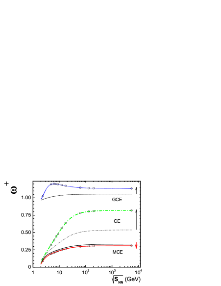
Figure 1: The scaled variances for negatively $\omega^{-}$ (left) and positively $\omega^{+}$ (right) charged particles. Both primordial and final $\omega^{\pm}$ are shown along the chemical freeze-out line for central Pb+Pb (Au+Au) collisions as the functions of the c.m. energy of the nucleon pair $\sqrt{s_{NN}}$. Different lines present the GCE, CE, and MCE results. Symbols at the lines for final particles correspond to the specific accelerator collision energies. The arrows show the effect of resonance decays.

At the chemical freeze-out of heavy-ion collisions, the Bose effect for pions and resonance decays are important and thus (see also Ref. [15]): $\omega^{-}_{g.c.e.}\cong 1.1$ and $\omega^{+}_{g.c.e.}\cong 1.2$ at the SPS energies. Note that in the Boltzmann approximation and neglecting the resonance decay effect one finds $\omega^{-}_{g.c.e.}=\omega^{+}_{g.c.e.}=1$.

Some qualitative features of the results should be mentioned. The effect of Bose and Fermi statistics is seen in primordial values in the GCE. At low temperatures most of positively charged hadrons are protons, and Fermi statistics dominates, $\omega^{+}_{g.c.e.}<1$. On the other hand, in the limit of high temperature (low $\mu_{B}/T$) most charged hadrons are pions and the effect of Bose statistics dominates, $\omega_{g.c.e.}^{\pm}>1$. Along the chemical freeze-out line, $\omega_{g.c.e.}^{-}$ is always slightly larger than 1, as $\pi^{-}$ mesons dominate at both low and high temperatures. The bump in $\omega^{+}_{g.c.e.}$ for final state particles seen in Fig. 1 at the small collision energies is due to a correlated production of proton and $\pi^{+}$ meson from $\Delta^{++}$ decays. This single resonance contribution dominates in $\omega^{+}_{g.c.e.}$ at small collision energies (small temperatures), but becomes relatively unimportant at the high collision energies.

A minimum in $\omega_{c.e.}^{-}$ for final particles is seen in Fig. 1. This is due to two effects. As the number of negatively charged particles is relatively small, $\langle N_{-}\rangle\ll\langle N_{+}\rangle$, at the low collision energies, both the CE suppression and the resonance decay effect are small. With increasing $\sqrt{s_{NN}}$, the CE effect alone leads to a decrease of $\omega^{-}_{c.e}$, but the resonance decay effect only leads to an increase of $\omega^{-}_{c.e}$. A combination of these two effects, the CE suppression and the resonance enhancement, leads to a minimum of $\omega^{-}_{c.e}$.

As expected, $\omega_{m.c.e.}<\omega_{c.e.}$, as an energy conservation further suppresses the particle number fluctuations. A new unexpected feature of the MCE is the suppression of the fluctuations after resonance decays. This is discussed in details in Ref. [16].

4 Comparison with NA49 Data

The scaled variance for the accepted particles is assumed to be equal to (see discussion of this point in Ref. [16]):

$$\omega~{}\equiv~{}\frac{\langle n^{2}\rangle~{}-~{}\langle n\rangle^{2}}{\langle n\rangle}~{}=~{}1~{}-~{}q~{}+q\cdot\omega_{4\pi}~{},$$ (13)

where $\omega_{4\pi}$ is the scaled variance for the full $4\pi$-acceptance. In the large acceptance limit ($q\approx 1$) the distribution of measured particles approaches the distribution in the full acceptance. For a very small acceptance ($q\approx 0$) the measured distribution approaches the Poisson one independent of the shape of the distribution in the full acceptance.

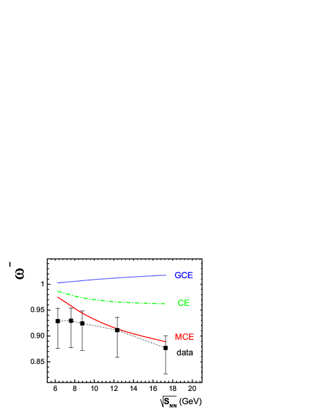
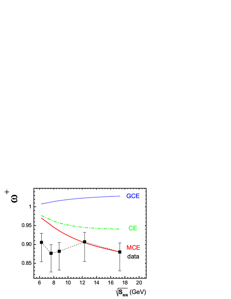
Figure 2: The scaled variances for negative (left) and positive (right) hadrons along the chemical freeze-out line for central Pb+Pb collisions at the SPS energies. The points show the preliminary data of NA49 [17]. Total (statistical+systematic) errors are indicated. The statistical model parameters $T$, $\mu_{B}$, and $\gamma_{S}$ at different SPS collision energies are taken at the chemical freeze-out, i.e. from fitting the hadron yields. Lines show the GCE, CE, and MCE results. The NA49 experimental acceptance is approximately taken into account according to Eq. (4.1).

The Fig. 2 presents the scaled variances $\omega^{-}$ and $\omega^{+}$ calculated with Eq. (13). The hadron-resonance gas calculations in the GCE, CE, and MCE shown in Fig. 1 are used for the $\omega_{4\pi}^{\pm}$. The NA49 acceptance used for the fluctuation measurements is located in the forward hemisphere [17]). The acceptance probabilities for positively and negatively charged hadrons are approximately equal, $q^{+}\approx q^{-}$, and the numerical values at different SPS energies are: $q^{\pm}=0.038,~{}0.063,$ $0.085,~{}0.131,~{}0.163$ at $\sqrt{s_{NN}}=6.27,~{}7.62,~{}8.77,~{}12.3,~{}17.3$ GeV, respectively. Eq. (13) has the following property: if $\omega_{4\pi}$ is smaller or larger than 1, the same inequality remains to be valid for $\omega$ at any value of $0<q\leq 1$. Thus one has a strong qualitative difference between the predictions of the statistical model valid for any freeze-out conditions and experimental acceptances. The CE and MCE correspond to $\omega_{m.c.e.}^{\pm}<\omega^{\pm}_{c.e.}<1$, and the GCE to $\omega_{g.c.e.}^{\pm}>1$.

From Fig. 2 it follows that the NA49 data for $\omega^{\pm}$ extracted from 1% of the most central Pb+Pb collisions at all SPS energies are best described by the results of the hadron-resonance gas model calculated within the MCE. The data reveal even stronger suppression of the particle number fluctuations. The chemical freeze-out parameters found at fixed collision energy have some uncertainties. However, the scaled variances $\omega_{m.c.e.}^{-}$ and $\omega_{m.c.e.}^{+}$ calculated in the full phase space within the MCE vary by less than 1% when changing the parameter set. In the NA49 acceptance the difference is almost completely washed out.

In order to allow for a detailed comparison of the distributions the ratio of the data and the model distributions to the Poisson one is presented in Fig. 3.

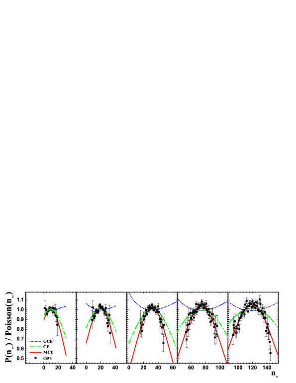
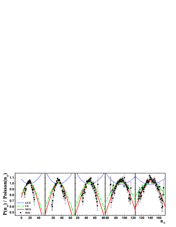
Figure 3: The ratio of the multiplicity distributions to Poisson ones for negatively (upper panel) and positively (lower panel) charged hadrons produced in central (1%) Pb+Pb collisions at 20$A$ GeV, 30$A$ GeV, 40$A$ GeV, 80$A$ GeV, and 158$A$ GeV (from left to right) in the NA49 acceptance [17]. The preliminary experimental data (solid points) of NA49 [17] are compared with the prediction of the hadron-resonance gas model obtained within different statistical ensembles, the GCE (dotted lines), the CE (dashed-dotted lines), and the MCE (solid lines).

The results for negatively and positively charged hadrons at 20$A$ GeV, 30$A$ GeV, 40$A$ GeV, 80$A$ GeV, and 158$A$ GeV are shown in Fig. 3. The convex shape of the data reflects the fact that the measured distribution is significantly narrower than the Poisson one. This suppression of fluctuations is observed for both charges, at all five SPS energies and it is consistent with the results for the scaled variance shown and discussed previously. The GCE hadron-resonance gas results are broader than the corresponding Poisson distribution. The ratio has a concave shape. An introduction of the quantum number conservation laws (the CE results) leads to the convex shape and significantly improves agreement with the data. Further improvement of the agreement is obtained by the additional introduction of the energy conservation law (the MCE results). The measured spectra surprisingly well agree with the MCE predictions.

5 Summary and Conclusions

The hadron multiplicity fluctuations in relativistic nucleus-nucleus collisions have been predicted in the statistical hadron-resonance gas model within the grand canonical, canonical, and micro-canonical ensembles in the thermodynamical limit. The microscopic correlator method has been extended to include three conserved charges – baryon number, electric charge, and strangeness – in the canonical ensemble, and additionally an energy conservation in the micro-canonical ensemble. The analytical formulas are used for the resonance decay contributions to the correlations and fluctuations. The scaled variances of negatively and positively charged particles for primordial and final state hadrons have been calculated at the chemical freeze-out in central Pb+Pb (Au+Au) collisions for different collision energies from SIS to LHC.

The effect of Bose enhancement and Fermi suppression can be seen in the primordial (before resonance decay) values of the scaled variances. The results presented in Fig. 1 demonstrate that the effects of quantum statistics are small at the chemical freeze-out. Resonance decays included into the GCE and CE lead to the enhancement of particle number fluctuations. An important feature of the MCE is the suppression of the fluctuations after resonance decays. This is discussed in details in Ref. [16].

A comparison of the multiplicity distributions and the scaled variances with the preliminary NA49 data on Pb+Pb collisions at the SPS energies has been done for the samples of about 1% of most central collisions selected by the number of projectile participants. This selection allows to eliminate effect of fluctuations of the number of nucleon participants. The effect of the limited experimental acceptance was taken into account by use of the uncorrelated particle approximation. The measured multiplicity distributions are significantly narrower than the Poisson one and allow to distinguish between model results derived within different statistical ensembles. The data surprisingly well agree with the expectations for the micro-canonical ensemble and exclude the canonical and grand-canonical ensembles. Thus, this is a first experimental observation of the predicted suppression [14, 15, 16] of the multiplicity fluctuations in relativistic gases in the thermodynamical limit due to conservation laws.

A validity of the micro-canonical description is surprising. In fact, significant event-by-event fluctuations of statistical model parameters may be expected. For instance, only a part of the total energy is available for the hadronization process. This part should be used in the hadron-resonance gas calculations while the remaining energy is contained in the collective motion of matter. The ratio between the hadronization and collective energies may vary from collision to collision and consequently increase the multiplicity fluctuations. The agreement between the data and the MCE predictions is even more surprising when the processes which are beyond the statistical hadron-resonance gas model are considered. Examples of these are jet and mini-jet production, heavy cluster formation, effects related to the phase transition or instabilities of the quark-gluon plasma. Naively all of them are expected to increase multiplicity fluctuations and thus lead to a disagreement between the data and the MCE predictions. A comparison of the data with the models which include these processes is obviously needed for significant conclusions.

On the model side there are, however, at least 2 additional effects which may lead to a suppression of the multiplicity fluctuations. The first of them follows from improving the description of the effect of the limited experimental acceptance within MCE [20]. The second one follows from taking into account the finite proper volume of hadrons. As shown in Ref. [21] the excluded volume effects lead to a reduction of the particle number fluctuations. The quantitative estimates of these two effects are needed.

More differential data on multiplicity fluctuations and correlations are required for further tests of the validity of the statistical models and observation of possible signals of the phase transitions. The experimental resolution in a measurement of the enhanced fluctuations due to the onset of deconfinement can be increased by increasing acceptance.

- [1] E. Fermi, Prog. Theor. Phys. 5, 570 (1950).
- [2] L. D. Landau, Izv. Akad. Nauk SSSR, Ser. Fiz. 17, 51 (1953).
- [3] R. Hagedorn, Nucl. Phys. B 24, 93 (1970).
- [4] For a recent review see Proceedings of the 3rd International Workshop: The Critical Point and Onset of Deconfinement, PoS(CPOD2006) (http://pos.sissa.it/), ed. F. Becattini, Firenze, Italy 3-6 July 2006.
- [5] J. Cleymans, H. Oeschler, K. Redlich, and S. Wheaton, Phys. Rev. C 73, 034905 (2006).
- [6] F. Becattini, J. Manninen, and M. Gaździcki, Phys. Rev. C 73, 044905 (2006).
- [7] A. Andronic, P. Braun-Munzinger, J. Stachel, Nucl. Phys. A 772, 167 (2006).
- [8] S.V. Afanasev et al., [NA49 Collaboration], Phys. Rev. Lett. 86, 1965 (2001); M.M. Aggarwal et al., [WA98 Collaboration], Phys. Rev. C 65, 054912 (2002); J. Adams et al., [STAR Collaboration], Phys. Rev. C 68, 044905 (2003); C. Roland et al., [NA49 Collaboration], J. Phys. G 30 S1381 (2004); Z.W. Chai et al., [PHOBOS Collaboration], J. Phys. Conf. Ser. 37, 128 (2005); M. Rybczynski et al. [NA49 Collaboration], J. Phys. Conf. Ser. 5, 74 (2005).
- [9] H. Appelshauser et al. [NA49 Collaboration], Phys. Lett. B 459, 679 (1999); D. Adamova et al., [CERES Collaboration], Nucl. Phys. A 727, 97 (2003); T. Anticic et al., [NA49 Collaboration], Phys. Rev. C 70, 034902 (2004); S.S. Adler et al., [PHENIX Collaboration], Phys. Rev. Lett. 93, 092301 (2004); J. Adams et al., [STAR Collaboration], Phys. Rev. C 71, 064906 (2005).
- [10] H. Heiselberg, Phys. Rep. 351, 161 (2001); S. Jeon and V. Koch, Review for Quark-Gluon Plasma 3, eds. R.C. Hwa and X.-N. Wang, World Scientific, Singapore, 430-490 (2004) [arXiv:hep-ph/0304012].
- [11] M. Gaździcki, M. I. Gorenstein, and St. Mrówczyński, Phys. Lett. B 585, 115 (2004); M. I. Gorenstein, M. Gazdźicki and O. S. Zozulya, Phys. Lett. B 585, 237 (2004).
- [12] I.N. Mishustin, Phys. Rev. Lett. 82, 4779 (1999); Nucl. Phys. A 681, 56c (2001); H. Heiselberg and A.D. Jackson, Phys. Rev. C 63, 064904 (2001).
- [13] M. Stephanov, K. Rajagopal, and E. Shuryak, Phys. Rev. Lett. 81, 4816 (1998); Phys. Rev. D 60, 114028 (1999); M. Stephanov, Acta Phys. Polon. B 35, 2939 (2004);
- [14] V.V. Begun, M. Gaździcki, M.I. Gorenstein, and O.S. Zozulya, Phys. Rev. C 70, 034901 (2004); V.V. Begun, M.I. Gorenstein, and O.S. Zozulya, Phys. Rev. C 72, 014902 (2005); A. Keränen, F. Becattini, V.V. Begun, M.I. Gorenstein, and O.S. Zozulya, J. Phys. G 31, S1095 (2005); F. Becattini, A. Keränen, L. Ferroni, and T. Gabbriellini, Phys. Rev. C 72, 064904 (2005); V.V. Begun, M.I. Gorenstein, A.P. Kostyuk, and O.S. Zozulya, Phys. Rev. C 71, 054904 (2005); J. Cleymans, K. Redlich, and L. Turko, Phys. Rev. C 71, 047902 (2005); J. Phys. G 31, 1421 (2005); V.V. Begun, M.I. Gorenstein, A.P. Kostyuk, and O.S. Zozulya, J. Phys. G 32, 935 (2006). V.V. Begun and M.I. Gorenstein, Phys. Rev. C 73, 054904 (2006).
- [15] V.V. Begun, M.I. Gorenstein, M. Hauer, V.P. Konchakovski, and O.S. Zozulya, Phys. Rev. C 74, 044903 (2006).
- [16] V.V. Begun, M. Gaździcki, M.I. Gorenstein, M. Hauer, V.P. Konchakovski, and B. Lungwitz, Phys. Rev. C 76, 024902 (2007).
- [17] B. Lungwitzt et al. [NA49 Collaboration], arXiv:nucl-ex/0610046.
- [18] S. Jeon and V. Koch, Phys. Rev. Lett. 83, 5435 (1999).
- [19] M. Hauer, V.V. Begun, and M.I. Gorenstein, nucl-th/0706.3290.
- [20] M. Hauer, to be published.
- [21] M.I. Gorenstein, M. Hauer and D. Nikolajenko, nucl-th/0702081 (Phys. Rev. C, to be published) .