The 191 orientable octahedral manifolds

Abstract

We enumerate all spaces obtained by gluing in pairs the faces of the octahedron in an orientation-reversing fashion. Whenever such a gluing gives rise to non-manifold points, we remove small open neighbourhoods of these points, so we actually deal with three-dimensional manifolds with (possibly empty) boundary.

There are 298 combinatorially inequivalent gluing patterns, and we show that they define 191 distinct manifolds, of which 132 are hyperbolic and 59 are not. All the 132 hyperbolic manifolds were already considered in different contexts by other authors, and we provide here their known “names” together with their main invariants. We also give the connected sum and JSJ decompositions for the 59 non-hyperbolic examples.

Our arguments make use of tools coming from hyperbolic geometry, together with quantum invariants and more classical techniques based on essential surfaces. Many (but not all) proofs were carried out by computer, but they do not involve issues of numerical accuracy.

MSC (2000): 57M50 (primary), 57M25 (secondary).

At the very beginning of his fundamental book [21], as an example of the richness of topology in three dimensions, Bill Thurston mentioned the fact that there are quite a few inequivalent ways of gluing together in pairs the faces of the octahedron. However, to our knowledge, as of today nobody had ever exactly determined the number of non-homeomorphic 3-manifolds arising as the results of these gluings. In this note we give a full solution to this problem, in the context of orientable (but unoriented) manifolds. After proving that there are 298 inequivalent gluing patterns, we have in fact proved the following:

Theorem 0.1.

Let $O$ be the octahedron and let ${\mathcal{O}}$ be the set of homeomorphism types of $3$-manifolds that can be obtained as follows:

• First, glue together in pairs in a simplicial and orientation-reversing fashion the faces of $O$, thus getting a compact polyhedron $X$;

• Second, remove from $X$ disjoint open stars of the non-manifold points, thus getting a compact orientable $3$-manifold with (possibly empty) boundary, all the components of which have positive genus.

Then ${\mathcal{O}}$ contains precisely $191$ elements, of which $132$ are hyperbolic and $59$ are not. More precisely, the numbers of inequivalent gluings and manifolds are split according to the topological type of the boundary as shown in Table 1, where $\Sigma_{g}$ denotes the orientable surface of genus $g$.

boundary type	$\#$(gluings)	hyperbolic	non-hyperbolic	total
$\emptyset$	37	–	17	17
$\Sigma_{1}$	81	$9$	$21$	30
$\Sigma_{1}\sqcup\Sigma_{1}$	9	2	5	7
$\Sigma_{2}$	113	63	16	79
$\Sigma_{2}\sqcup\Sigma_{1}$	2	2	–	2
$\Sigma_{3}$	56	56	–	56
Total	298	132	59	191

Table 1: Numbers of distinct manifolds arising from orientation-reversing gluings of the faces of an octahedron, with open stars of the non-manifold points removed

For the PL notions of polyhedron, manifold and star, see for instance [19]. As usual [1, 18, 21] a 3-manifold $M$ is “hyperbolic” if $M$ minus the boundary components of $M$ homeomorphic to the torus carries a complete metric with constant sectional curvatures $-1$ and totally geodesic boundary. The removed tori give rise to the so-called cusps of the manifold.

In addition to proving Theorem 0.1, we provide rather detailed information on the 191 elements of ${\mathcal{O}}$. In particular, we determine the volume and other invariants for the 132 hyperbolic manifolds in ${\mathcal{O}}$, and we identify the “names” they were given either in the Callahan-Hildebrand-Weeks census [2, 25] of small cusped hyperbolic manifolds, or in the Frigerio-Martelli-Petronio census [5, 6] of small hyperbolic manifolds with geodesic boundary. We also give detailed descriptions for the 59 non-hyperbolic elements of ${\mathcal{O}}$.

The question of counting the elements of ${\mathcal{O}}$ has a rather transparent combinatorial flavour and appears to be well-suited to computer investigation, but the complete answer would be extremely difficult to obtain without the aid of some rather sophisticated geometric tools developed over the last three decades by a number of mathematicians. It is indeed mostly thanks to hyperbolic geometry that one is able to show that certain gluings of $O$, despite being very similar to each other under many respects, are in fact distinct. This can be viewed as a manifestation of the crucial rôle played by hyperbolic geometry in the context of three-dimensional topology, as chiefly witnessed by Thurston’s geometrization, now apparently proved by Perelman [21, 15, 16, 17]

To prove Theorem 0.1 we have written some small specific Haskell code (to list the combinatorially inequivalent gluing patterns), and then we have used the “Orb” and “Manifold Recognizer” programs [9, 14]. There were however some manifolds the computer was unable to find hyperbolic structures for, and some pairs of manifolds that it was unable to tell apart. In these instances, we had to work by hand using classical techniques, including properly embedded essential surfaces. Despite being based on computers, our arguments do not involve issues of numerical accuracy, because approximation was only used within “Orb,” but the results were later checked through exact arithmetic in algebraic numbers fields with the program “Snap” [8].

Acknowledgements. Part of this work was carried out while the third-named author was visiting the University of Melbourne, the Université Paul Sabatier in Toulose and the Columbia University in New York. He is grateful to all these institutions for financial support, and he would like to thank Craig Hodgson, Michel Boileau and Dylan Thurston for their warm hospitality and inspiring mathematical discussions. The second named author was supported by the Marie Curie fellowship MIF1-CT-2006-038734.

1 Preliminaries

In this section we collect some elementary facts needed to prove Theorem 0.1.

Polyhedra vs manifolds

Given a gluing pattern $\varphi$ for the faces of the octahedron $O$, as described in the statement of Theorem 0.1, let us denote by $X(\varphi)$ the polyhedron resulting from the gluing, and by $M(\varphi)$ the 3-manifold obtained from $X(\varphi)$ by removing disjoint open stars of the non-manifold points. The following easy fact, that we leave to the reader, shows that $X(\varphi)$ and $M(\varphi)$ are in fact very tightly linked:

Proposition 1.1.

• Only the points of $X(\varphi)$ arising from the vertices of $O$ can be non-manifold points of $X(\varphi)$;

• The homeomorphism type of $X(\varphi)$ determines that of $M(\varphi)$, and conversely.

Before proceeding, recall that ${\mathcal{O}}$ denotes the set of homeomorphism classes of all $M(\varphi)$’s as $\varphi$ varies in the set simplicial and orientation-reversing gluing patterns of the faces of $O$.

Number of inequivalent gluings

To count the elements of ${\mathcal{O}}$, the first step is of course to enumerate the combinatorially inequivalent gluing patterns $\varphi$. Since $O$ has 8 faces and there are 3 different ways of gluing together any two chosen faces, the number of different patterns is $(8-1)!!\times 3^{4}=105\times 81=8505$. However there is a symmetry group with 48 elements acting on $O$, so the inequivalent patterns are actually much fewer than 8505. Using a small piece of Haskell code we have in fact shown the following:

Proposition 1.2.

There exist $298$ combinatorially inequivalent patterns of orientation-reversing gluings of the faces of $O$.

Classification according to boundary type

Two homeomorphic manifolds of course have homeomorphic boundaries. Moreover the boundary of an orientable 3-manifold is an orientable surface, which is very easy to identify by counting the number of connected components and computing the Euler characteristic of each of them. So the first easy step towards understanding ${\mathcal{O}}$ and proving Theorem 0.1 is to split the inequivalent gluing patterns according to the boundary they give rise to. Using again a Haskell program we found the results described in Table 2, where again $\Sigma_{g}$ denotes the orientable surface of genus $g$.

$\partial M(\varphi)$	$\#$(inequivalent $\varphi$’s)
$\emptyset$	37
$\Sigma_{1}$	81
$\Sigma_{1}\sqcup\Sigma_{1}$	9
$\Sigma_{2}$	113
$\Sigma_{2}\sqcup\Sigma_{1}$	2
$\Sigma_{3}$	56
Total	298

Table 2: Numbers of inequivalent gluings $\varphi$ of the faces of $O$, subdivided according to the topological type of $\partial M(\varphi)$

Further notation

Choosing one representative for each equivalence class of gluing patterns $\varphi$ and constructing the corresponding manifold $M(\varphi)$, we get a set of 298 manifolds that we denote henceforth by ${\mathcal{M}}$. By definition, ${\mathcal{O}}$ is obtained from ${\mathcal{M}}$ by identifying homeomorphic manifolds, and the main issue in establishing Theorem 0.1 is indeed to determine which elements of ${\mathcal{M}}$ are in fact homeomorphic to each other. Taking advantage of the easy work already described, we denote by ${\mathcal{M}}_{\Sigma}$ the set of elements of ${\mathcal{M}}$ having boundary $\Sigma$, thus getting a splitting of ${\mathcal{M}}$ as

$${\mathcal{M}}={\mathcal{M}}_{\emptyset}\sqcup{\mathcal{M}}_{\Sigma_{1}}\sqcup{\mathcal{M}}_{\Sigma_{1}\sqcup\Sigma_{1}}\sqcup{\mathcal{M}}_{\Sigma_{2}}\sqcup{\mathcal{M}}_{\Sigma_{2}\sqcup\Sigma_{1}}\sqcup{\mathcal{M}}_{\Sigma_{3}}.$$

Each set ${\mathcal{M}}_{\Sigma}$, after identifying homeomorphic manifolds, gives rise to some ${\mathcal{O}}_{\Sigma}$, that we further split as

$${\mathcal{O}}_{\Sigma}={\mathcal{O}}^{\mathrm{hyp}}_{\Sigma}\sqcup{\mathcal{O}}^{\mathrm{non}}_{\Sigma},$$

separating the hyperbolic members from the non-hyperbolic ones.

2 Hyperbolic manifolds

According to the well-known rigidity theorem [21, 1, 18], each $3$-manifold carries, up to isometry, at most one hyperbolic structure, as defined after the statement of Theorem 0.1. Note that the hyperbolic structures we consider are finite-volume by default. Moreover the following facts hold:

1. Every hyperbolic manifold with cusps or non-empty boundary has a “canonical decomposition,” which allows to efficiently compare it to any other such manifold. This is the decomposition into ideal polyhedra due to Epstein and Penner [3] for cusped manifolds (non-compact and without boundary), and the decomposition into truncated hyperideal polyhedra due to Kojima [11, 12] for manifolds with non-empty boundary. The hyperbolic structure of a manifold, whence (by rigidity) its topology, determines not only the polyhedral type of the blocks of the decomposition, but also the combinatorics of the gluings;

2. If a manifold is represented by a triangulation, namely as a gluing of tetrahedra, both its hyperbolic structure (if any) and its canonical decomposition can be searched algorithmically. This applies in particular to any element of the set ${\mathcal{M}}$ of manifolds we need to analyze, because the octahedron $O$ can be viewed as a partial gluing of 4 tetrahedra. The idea to construct the hyperbolic structure, due to Thurston [21], is to consider a space of parameters for the hyperbolic structures on each individual tetrahedron, and then to express the matching of the structures on the glued tetrahedra by a system of equations, that can be solved using numerical tools. The method for constructing the canonical decomposition is to modify any given geometric triangulation until the canonical decomposition is reached. This uses the “tilt formula” of Sakuma and Weeks [20] for cusped manifolds, and its variation due to Ushijima [23], together with some ideas from [7], for manifolds with non-empty geodesic boundary. Both the search for the hyperbolic structure and that for the canonical decomposition are not fully guaranteed to work, but in practice they always do (perhaps after some initial randomization of the triangulation);

3. The computer programs “SnapPea” [25] by Jeff Weeks, and “Orb” [9] by Damian Heard very efficiently implement the procedures mentioned in the previous point;

4. Both “SnapPea” and “Orb” employ numerical approximation, but the solutions these programs find can be checked using exact arithmetic in algebraic number fields with the program “Snap” [8] by Oliver Goodman.

Genus-3 geodesic boundary

To prove Theorem 0.1, for each of the 6 sets ${\mathcal{M}}_{\Sigma}$ we have, we need to determine which elements of ${\mathcal{M}}_{\Sigma}$ are homeomorphic to each other, thus finding the corresponding ${\mathcal{O}}_{\Sigma}$, and then to decide which elements of ${\mathcal{O}}_{\Sigma}$ are actually hyperbolic. We begin with the case $\Sigma=\Sigma_{3}$, where the result is quite striking. It was initially discovered from a computer experiment [5] and later established theoretically. We include a sketch of the proof for the sake of completeness.

Proposition 2.1.

The $56$ elements of ${\mathcal{M}}_{\Sigma_{3}}$ are all hyperbolic and distinct from each other, so ${\mathcal{O}}_{\Sigma_{3}}={\mathcal{O}}_{\Sigma_{3}}^{\mathrm{hyp}}={\mathcal{M}}_{\Sigma_{3}}$ has $56$ elements. For each element of this set the Kojima canonical decomposition has the same single block, namely a truncated regular hyperbolic octahedron with all dihedral angles equal to $\pi/6$.

Proof.

An easy computation of Euler characteristic shows that a gluing $\varphi$ defines a manifold $M(\varphi)$ bounded by $\Sigma_{3}$ if and only if it identifies all 12 edges to each other. We want to show that such an $M(\varphi)$ is hyperbolic with geodesic boundary by choosing a hyperbolic shape of the truncated octahedron that is matched by $\varphi$. Since all edges are glued together, this can only happen if the geometric shape is such that all edges have the same length, i.e. the octahedron is regular. If this is the case, all dihedral angles are also the same, so they must all be $2\pi/12$. Such an octahedron certainly does not exist in Euclidean or spherical geometry, but it does in hyperbolic geometry. This implies that $M(\varphi)$ is indeed hyperbolic.

Let us now analyze the Kojima canonical decomposition of $M(\varphi)$. To this end we recall [11, 12] that it is dual to the cut locus of the boundary, i.e. to the set of points having multiple shortest paths to $\partial M(\varphi)$. Using the fact that $M(\varphi)$ is the gluing of a regular truncated octahedron, which is totally symmetric, it is not too difficult to show that the Kojima decomposition is given by the octahedron itself, with its gluing pattern $\varphi$. This implies that the geometry of $M(\varphi)$, and hence its topology, determines $\varphi$. Therefore different $\varphi$’s give rise to different $M(\varphi)$’s. ∎

It follows from this result that the 56 elements of ${\mathcal{O}}_{\Sigma_{3}}^{\mathrm{hyp}}$ all have the same volume, that one can calculate to be $11.448776110...$ via Ushijima’s formulae [24]. Using “Orb” we have also computed the symmetry groups and homology of the elements of ${\mathcal{O}}_{\Sigma_{3}}^{\mathrm{hyp}}$, as described in Tables 3 and 4. Note that these invariants alone are far from sufficient to distinguish the 56 elements of ${\mathcal{M}}_{\Sigma_{3}}$ from each other. The tables also show the position of the manifolds in the file census$\_$4$\_$T3$\_$octa.snp available from [6]. Here and below ${\mathbb{Z}}_{n}$ and $D_{n}$ denote respectively the cyclic group with $n$ elements and the dihedral group with $2n$ elements.

File	no.	Volume	Sym	Hom
census$\_$4$\_$T3$\_$octa.snp	0	11.448776110	trivial	${\mathbb{Z}}^{3}$
census$\_$4$\_$T3$\_$octa.snp	1	11.448776110	trivial	${\mathbb{Z}}^{3}$
census$\_$4$\_$T3$\_$octa.snp	2	11.448776110	trivial	${\mathbb{Z}}^{3}$
census$\_$4$\_$T3$\_$octa.snp	3	11.448776110	trivial	${\mathbb{Z}}^{3}$
census$\_$4$\_$T3$\_$octa.snp	4	11.448776110	trivial	${\mathbb{Z}}^{3}$
census$\_$4$\_$T3$\_$octa.snp	5	11.448776110	trivial	${\mathbb{Z}}^{3}$
census$\_$4$\_$T3$\_$octa.snp	6	11.448776110	trivial	${\mathbb{Z}}^{3}$
census$\_$4$\_$T3$\_$octa.snp	7	11.448776110	trivial	${\mathbb{Z}}^{3}$
census$\_$4$\_$T3$\_$octa.snp	8	11.448776110	trivial	${\mathbb{Z}}^{3}$
census$\_$4$\_$T3$\_$octa.snp	9	11.448776110	trivial	${\mathbb{Z}}^{3}$
census$\_$4$\_$T3$\_$octa.snp	10	11.448776110	trivial	${\mathbb{Z}}^{3}$
census$\_$4$\_$T3$\_$octa.snp	11	11.448776110	trivial	${\mathbb{Z}}^{3}$
census$\_$4$\_$T3$\_$octa.snp	12	11.448776110	$D_{2}$	${\mathbb{Z}}^{3}$
census$\_$4$\_$T3$\_$octa.snp	13	11.448776110	${\mathbb{Z}}_{2}$	${\mathbb{Z}}^{3}$
census$\_$4$\_$T3$\_$octa.snp	14	11.448776110	${\mathbb{Z}}_{2}$	${\mathbb{Z}}^{3}$
census$\_$4$\_$T3$\_$octa.snp	15	11.448776110	trivial	${\mathbb{Z}}^{3}$
census$\_$4$\_$T3$\_$octa.snp	16	11.448776110	$D_{2}$	${\mathbb{Z}}^{3}$
census$\_$4$\_$T3$\_$octa.snp	17	11.448776110	${\mathbb{Z}}_{2}$	${\mathbb{Z}}^{3}$
census$\_$4$\_$T3$\_$octa.snp	18	11.448776110	$D_{4}$	${\mathbb{Z}}^{3}$
census$\_$4$\_$T3$\_$octa.snp	19	11.448776110	${\mathbb{Z}}_{2}$	${\mathbb{Z}}^{3}$
census$\_$4$\_$T3$\_$octa.snp	20	11.448776110	${\mathbb{Z}}_{2}$	${\mathbb{Z}}^{3}$
census$\_$4$\_$T3$\_$octa.snp	21	11.448776110	$D_{4}$	${\mathbb{Z}}^{3}$
census$\_$4$\_$T3$\_$octa.snp	22	11.448776110	${\mathbb{Z}}_{2}$	${\mathbb{Z}}^{3}$
census$\_$4$\_$T3$\_$octa.snp	23	11.448776110	${\mathbb{Z}}_{2}$	${\mathbb{Z}}^{3}$
census$\_$4$\_$T3$\_$octa.snp	24	11.448776110	${\mathbb{Z}}_{2}$	${\mathbb{Z}}^{3}$
census$\_$4$\_$T3$\_$octa.snp	25	11.448776110	trivial	${\mathbb{Z}}^{3}$
census$\_$4$\_$T3$\_$octa.snp	26	11.448776110	trivial	${\mathbb{Z}}^{3}$
census$\_$4$\_$T3$\_$octa.snp	27	11.448776110	trivial	${\mathbb{Z}}^{3}$
census$\_$4$\_$T3$\_$octa.snp	28	11.448776110	trivial	${\mathbb{Z}}^{3}$
census$\_$4$\_$T3$\_$octa.snp	29	11.448776110	trivial	${\mathbb{Z}}^{3}$
census$\_$4$\_$T3$\_$octa.snp	30	11.448776110	trivial	${\mathbb{Z}}^{3}$

Table 3: Information on the $56$ elements of ${\mathcal{O}}^{\mathrm{hyp}}_{\Sigma_{3}}$ (the compact orientable hyperbolic manifolds with geodesic boundary of genus $3$ arising from gluings of the octahedron) – part 1

File	no.	Volume	Sym	Hom
census$\_$4$\_$T3$\_$octa.snp	31	11.448776110	${\mathbb{Z}}_{2}$	${\mathbb{Z}}^{3}$
census$\_$4$\_$T3$\_$octa.snp	32	11.448776110	${\mathbb{Z}}_{2}$	${\mathbb{Z}}^{3}$
census$\_$4$\_$T3$\_$octa.snp	33	11.448776110	${\mathbb{Z}}_{2}$	${\mathbb{Z}}^{3}$
census$\_$4$\_$T3$\_$octa.snp	34	11.448776110	${\mathbb{Z}}_{2}$	${\mathbb{Z}}^{3}$
census$\_$4$\_$T3$\_$octa.snp	35	11.448776110	${\mathbb{Z}}_{2}$	${\mathbb{Z}}^{3}$
census$\_$4$\_$T3$\_$octa.snp	36	11.448776110	${\mathbb{Z}}_{2}$	${\mathbb{Z}}^{3}$
census$\_$4$\_$T3$\_$octa.snp	37	11.448776110	trivial	${\mathbb{Z}}_{3}+{\mathbb{Z}}^{3}$
census$\_$4$\_$T3$\_$octa.snp	38	11.448776110	${\mathbb{Z}}_{2}$	${\mathbb{Z}}_{3}+{\mathbb{Z}}^{3}$
census$\_$4$\_$T3$\_$octa.snp	39	11.448776110	$D_{2}$	${\mathbb{Z}}_{3}+{\mathbb{Z}}^{3}$
census$\_$4$\_$T3$\_$octa.snp	40	11.448776110	${\mathbb{Z}}_{4}$	${\mathbb{Z}}_{3}+{\mathbb{Z}}^{3}$
census$\_$4$\_$T3$\_$octa.snp	41	11.448776110	${\mathbb{Z}}_{2}$	${\mathbb{Z}}^{3}$
census$\_$4$\_$T3$\_$octa.snp	42	11.448776110	trivial	${\mathbb{Z}}^{3}$
census$\_$4$\_$T3$\_$octa.snp	43	11.448776110	${\mathbb{Z}}_{2}$	${\mathbb{Z}}^{3}$
census$\_$4$\_$T3$\_$octa.snp	44	11.448776110	${\mathbb{Z}}_{2}$	${\mathbb{Z}}^{3}$
census$\_$4$\_$T3$\_$octa.snp	45	11.448776110	${\mathbb{Z}}_{2}$	${\mathbb{Z}}^{3}$
census$\_$4$\_$T3$\_$octa.snp	46	11.448776110	trivial	${\mathbb{Z}}^{3}$
census$\_$4$\_$T3$\_$octa.snp	47	11.448776110	trivial	${\mathbb{Z}}^{3}$
census$\_$4$\_$T3$\_$octa.snp	48	11.448776110	${\mathbb{Z}}_{2}$	${\mathbb{Z}}^{3}$
census$\_$4$\_$T3$\_$octa.snp	49	11.448776110	trivial	${\mathbb{Z}}^{3}$
census$\_$4$\_$T3$\_$octa.snp	50	11.448776110	${\mathbb{Z}}_{2}$	${\mathbb{Z}}^{3}$
census$\_$4$\_$T3$\_$octa.snp	51	11.448776110	trivial	${\mathbb{Z}}^{3}$
census$\_$4$\_$T3$\_$octa.snp	52	11.448776110	trivial	${\mathbb{Z}}^{3}$
census$\_$4$\_$T3$\_$octa.snp	53	11.448776110	trivial	${\mathbb{Z}}^{3}$
census$\_$4$\_$T3$\_$octa.snp	54	11.448776110	${\mathbb{Z}}_{2}$	${\mathbb{Z}}^{3}$
census$\_$4$\_$T3$\_$octa.snp	55	11.448776110	${\mathbb{Z}}_{2}$	${\mathbb{Z}}^{3}$

Table 4: Information on the $56$ elements of ${\mathcal{O}}^{\mathrm{hyp}}_{\Sigma_{3}}$ (the compact orientable hyperbolic manifolds with geodesic boundary of genus $3$ arising from gluings of the octahedron) – part 2

Genus-2 geodesic boundary and one cusp

For the case $\Sigma=\Sigma_{2}\sqcup\Sigma_{1}$ the analysis of ${\mathcal{M}}_{\Sigma}$ was already contained in [5]:

Proposition 2.2.

The two elements of ${\mathcal{M}}_{\Sigma_{2}\sqcup\Sigma_{1}}$ are hyperbolic and distinct from each other, so ${\mathcal{O}}_{\Sigma_{2}\sqcup\Sigma_{1}}={\mathcal{O}}_{\Sigma_{2}\sqcup\Sigma_{1}}^{\mathrm{hyp}}={\mathcal{M}}_{\Sigma_{2}\sqcup\Sigma_{1}}$ has two elements.

Table 5 describes the symmetry group and homology of both elements of ${\mathcal{O}}_{\Sigma_{2}\sqcup\Sigma_{1}}^{\mathrm{hyp}}$, and reference to their position in the files available from [6], as we determined using “Orb”.

File	no.	Volume	Sym	Hom
census$\_$4$\_$cusp.snp	14	8.681737155	${\mathbb{Z}}_{2}$	${\mathbb{Z}}^{3}$
census$\_$4$\_$cusp.snp	15	8.681737155	${\mathbb{Z}}_{2}$	${\mathbb{Z}}^{3}$

Table 5: Information on the $2$ elements of ${\mathcal{O}}^{\mathrm{hyp}}_{\Sigma_{2}\sqcup\Sigma_{1}}$ (the orientable hyperbolic manifolds with one cusp and geodesic boundary of genus 2 arising from gluings of the octahedron)

Genus-2 geodesic boundary

The following partial information on the elements of ${\mathcal{M}}_{\Sigma_{2}}$ can be deduced from the results in [5]:

Proposition 2.3.

The set ${\mathcal{M}}_{\Sigma_{2}}$ (which has $113$ elements) contains the following subsets:

• A set of $14$ distinct hyperbolic manifolds with Kojima decomposition having one and the same block, namely a regular truncated octahedron with all dihedral angles equal to $\pi/3$;

• A set of $8$ distinct hyperbolic manifolds with Kojima decomposition having one and the same block, namely a non-regular truncated octahedron;

• A set of $4$ distinct hyperbolic manifolds with Kojima decomposition having the same two blocks, namely two identical square pyramids.

Moreover any other hyperbolic element of ${\mathcal{M}}_{\Sigma_{2}}$ has Kojima decomposition consisting of tetrahedra only.

To complete the analysis of the hyperbolic elements of ${\mathcal{M}}_{\Sigma_{2}}$, using “Orb” (and then “Snap” for a formal verification) we proved the following:

Proposition 2.4.

Of the $113-(14+8+4)=87$ elements of ${\mathcal{M}}_{\Sigma_{2}}$ not covered by Proposition 2.3, at least $37$ are hyperbolic, and they are all distinct from each other.

After “Orb” has been able to construct the hyperbolic structure of an element $M$ of ${\mathcal{M}}$ and the solution has been checked using “Snap,” one can state for sure that $M$ is indeed hyperbolic, and one can positively determine whether $M$ is homeomorphic to any other given hyperbolic manifold. However if “Orb” fails to construct the structure one has to prove by some other method that $M$ is actually non-hyperbolic. This is what we do in the next section. In particular, we prove that the $113-[(14+8+4)+37]=50$ elements of ${\mathcal{M}}_{\Sigma_{2}}$ not covered by Propositions 2.3 and 2.4 are indeed non-hyperbolic, which implies the following:

Proposition 2.5.

The set ${\mathcal{O}}^{\mathrm{hyp}}_{\Sigma_{2}}$ consists of the $63$ manifolds described in Propositions 2.3 and 2.4.

The elements of ${\mathcal{O}}^{\mathrm{hyp}}_{\Sigma_{2}}$, together with the usual information on them determined by “Orb,” are listed in order of increasing volume in Tables 6 and 7. Again the first column indicates the file from [6] where the manifold can be located in the position (starting from 0) specified in the second column. Note that the name of the file contains a description of the Kojima canonical decomposition (e.g. tetra6 means that this decomposition consists of 6 tetrahedra).

File	no.	Volume	Sym	Hom
census$\_$3.snp	93	7.636519630	${\mathbb{Z}}_{2}$	${\mathbb{Z}}^{2}$
census$\_$3.snp	90	7.636519630	${\mathbb{Z}}_{2}$	${\mathbb{Z}}^{2}$
census$\_$3.snp	89	7.636519630	${\mathbb{Z}}_{2}$	${\mathbb{Z}}^{2}$
census$\_$3.snp	88	7.636519630	${\mathbb{Z}}_{2}$	${\mathbb{Z}}^{2}$
census$\_$3.snp	92	7.636519630	trivial	${\mathbb{Z}}^{2}$
census$\_$3.snp	86	7.636519630	trivial	${\mathbb{Z}}^{2}$
census$\_$3.snp	87	7.636519630	${\mathbb{Z}}_{2}$	${\mathbb{Z}}^{2}$
census$\_$3.snp	94	7.636519630	${\mathbb{Z}}_{2}$	${\mathbb{Z}}^{2}$
census$\_$3.snp	91	7.636519630	${\mathbb{Z}}_{2}$	${\mathbb{Z}}^{2}$
census$\_$4$\_$T2$\_$tetra6.snp	2	8.297977385	${\mathbb{Z}}_{2}$	${\mathbb{Z}}^{2}$
census$\_$4$\_$T2$\_$tetra6.snp	1	8.297977385	${\mathbb{Z}}_{2}$	${\mathbb{Z}}^{2}$
census$\_$4$\_$T2$\_$tetra6.snp	0	8.297977385	${\mathbb{Z}}_{2}$	${\mathbb{Z}}^{2}$
census$\_$4$\_$T2$\_$tetra4.snp	75	8.625848296	${\mathbb{Z}}_{2}$	${\mathbb{Z}}^{2}$
census$\_$4$\_$T2$\_$tetra4.snp	76	8.625848296	${\mathbb{Z}}_{2}$	${\mathbb{Z}}^{2}$
census$\_$4$\_$T2$\_$octa$\_$nonreg.snp	1	8.739252140	$D_{3}$	${\mathbb{Z}}_{3}+{\mathbb{Z}}^{2}$
census$\_$4$\_$T2$\_$octa$\_$nonreg.snp	0	8.739252140	$D_{3}$	${\mathbb{Z}}_{3}+{\mathbb{Z}}^{2}$
census$\_$4$\_$T2$\_$octa$\_$nonreg.snp	7	8.739252140	$D_{3}$	${\mathbb{Z}}_{3}+{\mathbb{Z}}^{2}$
census$\_$4$\_$T2$\_$octa$\_$nonreg.snp	6	8.739252140	$D_{3}$	${\mathbb{Z}}_{3}+{\mathbb{Z}}^{2}$
census$\_$4$\_$T2$\_$octa$\_$nonreg.snp	2	8.739252140	${\mathbb{Z}}_{2}$	${\mathbb{Z}}^{2}$
census$\_$4$\_$T2$\_$octa$\_$nonreg.snp	5	8.739252140	${\mathbb{Z}}_{2}$	${\mathbb{Z}}^{2}$
census$\_$4$\_$T2$\_$octa$\_$nonreg.snp	4	8.739252140	${\mathbb{Z}}_{2}$	${\mathbb{Z}}^{2}$
census$\_$4$\_$T2$\_$octa$\_$nonreg.snp	3	8.739252140	${\mathbb{Z}}_{2}$	${\mathbb{Z}}^{2}$
census$\_$4$\_$T2$\_$pyramids.snp	2	9.044841574	${\mathbb{Z}}_{2}$	${\mathbb{Z}}^{2}$
census$\_$4$\_$T2$\_$pyramids.snp	1	9.044841574	${\mathbb{Z}}_{2}$	${\mathbb{Z}}^{2}$
census$\_$4$\_$T2$\_$pyramids.snp	0	9.044841574	${\mathbb{Z}}_{2}$	${\mathbb{Z}}^{2}$
census$\_$4$\_$T2$\_$pyramids.snp	3	9.044841574	${\mathbb{Z}}_{2}$	${\mathbb{Z}}^{2}$
census$\_$4$\_$T2$\_$tetra4.snp	161	9.082538547	trivial	${\mathbb{Z}}^{2}$
census$\_$4$\_$T2$\_$tetra4.snp	162	9.082538547	trivial	${\mathbb{Z}}^{2}$
census$\_$4$\_$T2$\_$tetra4.snp	166	9.087925790	${\mathbb{Z}}_{2}$	${\mathbb{Z}}^{2}$
census$\_$4$\_$T2$\_$tetra4.snp	165	9.087925790	${\mathbb{Z}}_{2}$	${\mathbb{Z}}^{2}$
census$\_$4$\_$T2$\_$tetra4.snp	163	9.087925790	${\mathbb{Z}}_{2}$	${\mathbb{Z}}_{3}+{\mathbb{Z}}^{2}$
census$\_$4$\_$T2$\_$tetra4.snp	164	9.087925790	${\mathbb{Z}}_{2}$	${\mathbb{Z}}_{3}+{\mathbb{Z}}^{2}$

Table 6: Information on the $63$ elements of ${\mathcal{O}}^{\mathrm{hyp}}_{\Sigma_{2}}$ (the compact orientable hyperbolic manifolds with geodesic boundary of genus $2$ arising from gluings of the octahedron) – part 1

File	no.	Volume	Sym	Hom
census$\_$4$\_$T2$\_$tetra5.snp	4	9.134474458	$D_{4}$	${\mathbb{Z}}^{3}$
census$\_$4$\_$T2$\_$tetra5.snp	3	9.134474458	${\mathbb{Z}}_{2}$	${\mathbb{Z}}_{2}+{\mathbb{Z}}^{2}$
census$\_$4$\_$T2$\_$tetra5.snp	7	9.134474458	${\mathbb{Z}}_{2}$	${\mathbb{Z}}_{2}+{\mathbb{Z}}^{2}$
census$\_$4$\_$T2$\_$tetra5.snp	5	9.134474458	$D_{4}$	${\mathbb{Z}}^{3}$
census$\_$4$\_$T2$\_$tetra5.snp	6	9.134474458	$D_{2}$	${\mathbb{Z}}_{2}+{\mathbb{Z}}^{2}$
census$\_$4$\_$T2$\_$tetra5.snp	8	9.134474458	$D_{2}$	${\mathbb{Z}}_{2}+{\mathbb{Z}}^{2}$
census$\_$4$\_$T2$\_$tetra5.snp	15	9.333442928	${\mathbb{Z}}_{2}$	${\mathbb{Z}}^{2}$
census$\_$4$\_$T2$\_$tetra5.snp	18	9.333442928	${\mathbb{Z}}_{2}$	${\mathbb{Z}}^{2}$
census$\_$4$\_$T2$\_$tetra5.snp	16	9.333442928	trivial	${\mathbb{Z}}^{2}$
census$\_$4$\_$T2$\_$tetra5.snp	19	9.333442928	${\mathbb{Z}}_{2}$	${\mathbb{Z}}_{3}+{\mathbb{Z}}^{2}$
census$\_$4$\_$T2$\_$tetra5.snp	17	9.333442928	trivial	${\mathbb{Z}}^{2}$
census$\_$4$\_$T2$\_$tetra5.snp	20	9.333442928	${\mathbb{Z}}_{2}$	${\mathbb{Z}}_{3}+{\mathbb{Z}}^{2}$
census$\_$4$\_$T2$\_$tetra4.snp	246	9.346204962	trivial	${\mathbb{Z}}^{2}$
census$\_$4$\_$T2$\_$tetra4.snp	245	9.346204962	${\mathbb{Z}}_{2}$	${\mathbb{Z}}_{3}+{\mathbb{Z}}^{2}$
census$\_$4$\_$T2$\_$tetra4.snp	247	9.346204962	${\mathbb{Z}}_{2}$	${\mathbb{Z}}^{2}$
census$\_$4$\_$T2$\_$tetra5.snp	21	9.350261353	${\mathbb{Z}}_{2}$	${\mathbb{Z}}_{3}+{\mathbb{Z}}^{2}$
census$\_$4$\_$T2$\_$tetra5.snp	22	9.350261353	${\mathbb{Z}}_{2}$	${\mathbb{Z}}^{2}$
census$\_$4$\_$T2$\_$octa$\_$reg.snp	11	9.415841683	$D_{2}$	${\mathbb{Z}}^{2}$
census$\_$4$\_$T2$\_$octa$\_$reg.snp	5	9.415841683	${\mathbb{Z}}_{2}$	${\mathbb{Z}}/2+{\mathbb{Z}}^{2}$
census$\_$4$\_$T2$\_$octa$\_$reg.snp	1	9.415841683	$D_{4}$	${\mathbb{Z}}/3+{\mathbb{Z}}^{2}$
census$\_$4$\_$T2$\_$octa$\_$reg.snp	9	9.415841683	${\mathbb{Z}}_{2}+{\mathbb{Z}}_{4}$	${\mathbb{Z}}_{5}+{\mathbb{Z}}^{2}$
census$\_$4$\_$T2$\_$octa$\_$reg.snp	6	9.415841683	$D_{3}$	${\mathbb{Z}}_{6}+{\mathbb{Z}}^{2}$
census$\_$4$\_$T2$\_$octa$\_$reg.snp	7	9.415841683	$D_{3}$	${\mathbb{Z}}_{6}+{\mathbb{Z}}^{2}$
census$\_$4$\_$T2$\_$octa$\_$reg.snp	4	9.415841683	${\mathbb{Z}}_{2}$	${\mathbb{Z}}_{2}+{\mathbb{Z}}^{2}$
census$\_$4$\_$T2$\_$octa$\_$reg.snp	3	9.415841683	trivial	${\mathbb{Z}}_{2}+{\mathbb{Z}}^{2}$
census$\_$4$\_$T2$\_$octa$\_$reg.snp	10	9.415841683	$D_{4}$	${\mathbb{Z}}^{2}$
census$\_$4$\_$T2$\_$octa$\_$reg.snp	8	9.415841683	trivial	${\mathbb{Z}}_{2}+{\mathbb{Z}}^{2}$
census$\_$4$\_$T2$\_$octa$\_$reg.snp	13	9.415841683	trivial	${\mathbb{Z}}^{2}$
census$\_$4$\_$T2$\_$octa$\_$reg.snp	2	9.415841683	$D_{2}$	${\mathbb{Z}}^{2}$
census$\_$4$\_$T2$\_$octa$\_$reg.snp	12	9.415841683	${\mathbb{Z}}_{4}$	${\mathbb{Z}}^{2}$
census$\_$4$\_$T2$\_$octa$\_$reg.snp	0	9.415841683	$D_{2}$	${\mathbb{Z}}_{3}+{\mathbb{Z}}^{2}$

Table 7: Information on the $63$ elements of ${\mathcal{O}}^{\mathrm{hyp}}_{\Sigma_{2}}$ (the compact orientable hyperbolic manifolds with geodesic boundary of genus $2$ arising from gluings of the octahedron) – part 2

Cusped manifolds

We carried out the analysis of the hyperbolic elements of ${\mathcal{M}}_{\Sigma_{1}}$ and ${\mathcal{M}}_{\Sigma_{1}\sqcup\Sigma_{1}}$ using “Orb,” with the following result:

Proposition 2.6.

• The set ${\mathcal{M}}_{\Sigma_{1}}$ (which has $81$ elements) contains $11$ hyperbolic manifolds, yielding $9$ distinct homeomorphism types;

• The set ${\mathcal{M}}_{\Sigma_{1}\sqcup\Sigma_{1}}$ (which has $9$ elements) contains $2$ distinct hyperbolic manifolds.

As above for the case of boundary $\Sigma_{2}$, failure of “Orb” to find a cusped hyperbolic structure does not imply that the structure does not exist. However in the next section we show that the $81-11=70$ elements of ${\mathcal{M}}_{\Sigma_{1}}$ and the $9-2=7$ elements of ${\mathcal{M}}_{\Sigma_{1}\sqcup\Sigma_{1}}$ not covered by Proposition 2.6 are indeed non-hyperbolic, which implies the following:

Proposition 2.7.

The set ${\mathcal{O}}^{\mathrm{hyp}}_{\Sigma_{1}}$ (respectively, ${\mathcal{O}}^{\mathrm{hyp}}_{\Sigma_{1}\sqcup\Sigma_{1}}$) consists of the $9$ (respectively, $2$) manifolds described in Proposition 2.6.

Using “Orb” we have determined the symmetry group and homology of each element of ${\mathcal{O}}^{\mathrm{hyp}}_{\Sigma_{1}}$ and ${\mathcal{O}}^{\mathrm{hyp}}_{\Sigma_{1}\sqcup\Sigma_{1}}$, together with the name it was given in [2, 25]. This information appears in Tables 8 and 9.

Name	Volume	Sym	Hom
m006	2.568970601	$D_{2}$	${\mathbb{Z}}_{5}+{\mathbb{Z}}$
m007	2.568970601	$D_{2}$	${\mathbb{Z}}_{3}+{\mathbb{Z}}$
m009	2.666744783	$D_{2}$	${\mathbb{Z}}_{2}+{\mathbb{Z}}$
m010	2.666744783	$D_{2}$	${\mathbb{Z}}_{6}+{\mathbb{Z}}$
m011	2.781833912	${\mathbb{Z}}$	${\mathbb{Z}}_{2}$
m032	3.163963229	$D_{2}$	${\mathbb{Z}}$
m033	3.163963229	$D_{2}$	${\mathbb{Z}}_{9}+{\mathbb{Z}}$
m036	3.177293279	$D_{2}$	${\mathbb{Z}}_{3}+{\mathbb{Z}}$
m038	3.177293279	$D_{2}$	${\mathbb{Z}}$

Table 8: Information on the $9$ elements of ${\mathcal{O}}^{\mathrm{hyp}}_{\Sigma_{1}}$ (the one-cusped orientable hyperbolic manifolds arising from gluings of the octahedron)

Name	Volume	Sym	Hom
m125	3.663862377	$D_{4}$	${\mathbb{Z}}^{2}$
m129	3.663862377	$D_{4}$	${\mathbb{Z}}^{2}$

Table 9: Information on the $2$ elements of ${\mathcal{O}}^{\mathrm{hyp}}_{\Sigma_{1}\sqcup\Sigma_{1}}$ (the two-cusped orientable hyperbolic manifolds arising from gluings of the octahedron)

3 Non-hyperbolic manifolds

In this section we analyze the elements of ${\mathcal{M}}$ not covered by Propositions 2.1, 2.2, 2.3, 2.4, and 2.6, thus completing our enumeration of ${\mathcal{O}}$. Recall that only ${\mathcal{M}}_{\emptyset}$, ${\mathcal{M}}_{\Sigma_{1}}$, ${\mathcal{M}}_{\Sigma_{1}\sqcup\Sigma_{1}}$, and ${\mathcal{M}}_{\Sigma_{2}}$ still require some work.

Matching of triangulations

The numbers of elements of ${\mathcal{M}}_{\Sigma}$ not already recognized to belong to ${\mathcal{O}}^{\mathrm{hyp}}_{\Sigma}$ are as described in the central column of Table 10. As already remarked, all these manifolds come with a triangulation consisting of 4 tetrahedra. Now, one of the features of “Orb” is to compare two triangulated manifolds for equality by randomizing the initial triangulations and matching. So we have first exploited this feature to reduce the numbers of potentially distinct homeomorphism types, getting the results described in the right column of Table 10. In the rest of this section we describe the proof of the following result:

type according	apparently	apparently distinct
to the boundary	non-hyperbolic	after matching
${\mathcal{M}}_{\emptyset}$	37	17
${\mathcal{M}}_{\Sigma_{1}}$	70	21
${\mathcal{M}}_{\Sigma_{1}\sqcup\Sigma_{1}}$	7	5
${\mathcal{M}}_{\Sigma_{2}}$	50	16
${\mathcal{M}}_{\Sigma_{2}\sqcup\Sigma_{1}}$	–	–
${\mathcal{M}}_{\Sigma_{3}}$	–	–

Table 10: Numbers of apparently non-hyperbolic elements of ${\mathcal{M}}$, and potentially distinct homeomorphism types after the triangulation matching performed using “Orb”

Proposition 3.1.

For $\Sigma=\emptyset,\Sigma_{1},\Sigma_{1}\sqcup\Sigma_{1},\Sigma_{2}$ and $I=17,21,5,16$, respectively, let $\big{(}M_{\Sigma}^{(i)}\big{)}_{i=1}^{I}$ be the manifolds as in the right column of Table 10. Then:

1. If $i\neq j$ then $M_{\Sigma}^{(i)}$ is not homeomorphic to $M_{\Sigma}^{(j)}$;

2. Each $M_{\Sigma}^{(i)}$ is non-hyperbolic.

This implies Propositions 2.5 and 2.7, the equalities ${\mathcal{O}}^{\mathrm{non}}_{\Sigma}=\big{(}M_{\Sigma}^{(i)}\big{)}_{i=1}^{I}$ for all four relevant $\Sigma$’s, and hence Theorem 0.1. Our proof utilizes computers and theoretical work. Note that Proposition 3.1 shows that “Orb” was totally efficient both in constructing the hyperbolic structures and in comparing the non-hyperbolic manifolds for homeomorphism.

In the sequel we freely use several classical notions, results and techniques of 3-manifold topology, in particular the definition of essential surface, the Haken-Kneser-Milnor decomposition along spheres, the definition and properties of Seifert fibred spaces, and the Jaco-Shalen-Johansson decomposition along tori and annuli, see [10, 4, 13]. Moreover we use the fact that if a manifold contains a properly embedded essential surface with non-negative Euler characteristic then the manifold cannot be hyperbolic.

The “3-Manifold Recognizer”

As already mentioned, besides “Orb” we have employed another software, namely the “3-Manifold Recognizer,” written by Tarkaev and Matveev [14]. The input to this program is a triangulation of a 3-manifold $M$ and its output is the “name” of $M$, by which we mean the following:

• For a Seifert $M$, (one of) its Seifert structure(s);

• For a hyperbolic $M$, its presentation(s) as a Dehn filling of a manifold in the tables of Weeks [2];

• For an irreducible $M$ having JSJ decomposition into more than one block, the names (as just illustrated) of the blocks, together with the gluing instructions between the blocks;

• For a reducible manifold, the names (as just illustrated) of its irreducible summands.

The program is not guaranteed to always find the name of the manifold (for instance, it does not even attempt to do this for manifolds with boundary of genus 2 or more, and it happens to fail also in other cases). But it can always compute the first homology and, in the case of boundary of genus at most $1$, the Turaev-Viro invariants [22], which turned out to be very useful for us.

We now describe the proof of Proposition 3.1, breaking it into separate paragraphs according to the boundary type $\Sigma$, and at the same time we provide detailed topological information on the manifolds $M_{\Sigma}^{(i)}$.

Closed manifolds

Let us start with the case $\Sigma=\emptyset$. The second item in Proposition 3.1, namely the proof that each $M_{\emptyset}^{(i)}$ is non-hyperbolic, was not an issue in this case. In fact, it has been known for a long time [13] that any triangulation of a closed hyperbolic manifold contains at least 9 tetrahedra, whereas each $M_{\emptyset}^{(i)}$ admits a triangulation with 4 tetrahedra.

To show that $M_{\emptyset}^{(i)}\not\cong M_{\emptyset}^{(j)}$ for $1\leqslant i<j\leqslant 17$ we have run the “Recognizer,” that successfully identified all the manifolds (this was also independently done by Tarkaev). From the names (all manifolds turned out to be Seifert or connected sums of Seifert) we could see that the $M_{\emptyset}^{(i)}$’s were indeed all distinct, except possibly for $M_{\emptyset}^{(1)}$ and $M_{\emptyset}^{(2)}$, that were both recognized to be the connected sum of two copies of the lens space $L(3,1)$. Since $L(3,1)$ has no orientation-reversing automorphism, even if one looks (as we do) at orientable but unoriented manifolds, there are two distinct ways of performing the connected sum of $L(3,1)$ with itself, so the names of $M_{\emptyset}^{(1)}$ and $M_{\emptyset}^{(2)}$ provided by the “Recognizer” were indeed ambiguous.

To show that $M_{\emptyset}^{(1)}\not\cong M_{\emptyset}^{(2)}$ we then had to examine their triangulations by hand, introducing an arbitrary orientation on each and finding the essential sphere realizing the connected sum. Cutting along this sphere and capping off, we saw that for $M_{\emptyset}^{(1)}$ the two connected summands were distinctly oriented copies of $L(3,1)$, while for $M_{\emptyset}^{(2)}$ they were consistently oriented. This led us to the proof of Proposition 3.1 for $\Sigma=\emptyset$. More precisely we established the following:

Proposition 3.2.

The set $\mathcal{O}^{\mathrm{non}}_{\emptyset}$ consists of $13$ irreducible manifolds and $4$ reducible ones. The irreducible manifolds are the Seifert spaces

$${\mathbb{S}}^{3},\qquad{\mathbb{P}}^{3},\qquad{\mathbb{S}}^{2}\times{\mathbb{S}}^{1},\qquad L(3,1),\qquad L(4,1),\qquad L(5,2),$$

$$L(6,1),\qquad L(9,2),\qquad L(12,5),\qquad\big{(}{\mathbb{P}}^{2};(3,2),(1,0)\big{)},$$

$$\big{(}{\mathbb{P}}^{2};(2,1),(1,1)\big{)},\qquad\big{(}{\mathbb{P}}^{2};(1,3)\big{)},\qquad\big{(}{\mathbb{S}}^{2};(2,1),(3,1),(3,1),(1,-1)\big{)},$$

and the reducible ones are

$${\mathbb{P}}^{3}\#{\mathbb{P}}^{3},\qquad{\mathbb{P}}^{3}\#L(3,1),\qquad L(3,1)\#L(3,1),\qquad L(3,1)\#\big{(}-L(3,1)\big{)}.$$

One-cusped manifolds

In this case both items in Proposition 3.1 required some work. We proceeded as follows.

To prove that $M_{\Sigma_{1}}^{(i)}\not\cong M_{\Sigma_{1}}^{(j)}$ for $1\leqslant i<j\leqslant 21$ we again employed the “Recognizer”, using which we calculated the first homology group and Turaev-Viro invariants up to order 16 of each $M_{\Sigma_{1}}^{(i)}$. From this computation we deduced that $M_{\Sigma_{1}}^{(i)}\not\cong M_{\Sigma_{1}}^{(j)}$ for $1\leqslant i<j\leqslant 21$ except possibly for $i=1,2,3,4$ and $j=i+4$. For the four pairs of manifolds left, we showed the homeomorphism was impossible by analyzing the JSJ decompositions. Specifically, $M_{\Sigma_{1}}^{(1)}$ and $M_{\Sigma_{1}}^{(5)}$ turned out to be Seifert and distinct, and the same happened for $M_{\Sigma_{1}}^{(2)}$ and $M_{\Sigma_{1}}^{(6)}$, whereas $M_{\Sigma_{1}}^{(3)}$ and $M_{\Sigma_{1}}^{(7)}$ had non-trivial JSJ decompositions, with the same blocks but different gluing matrices, and analogously for $M_{\Sigma_{1}}^{(4)}$ and $M_{\Sigma_{1}}^{(8)}$.

The results just described allowed us to conclude that $M_{\Sigma_{1}}^{(i)}$ is non-hyperbolic for $i=1,\ldots,8$. To show that the same holds for $i=9,\ldots,21$ we used the “Recognizer” again to compute connected sum and JSJ decompositions. In each instance the desired result was returned because we obtained either connected sums or manifolds having JSJ decomposition consisting of Seifert pieces (sometimes only one of them). It is perhaps worth mentioning that in one case the “Recognizer” failed to return the answer right away, but we were able to transform the triangulation by hand into one that the “Recognizer” could handle.

These arguments led us to the proof of Proposition 3.1 for the case $\Sigma=\Sigma_{1}$, and also to the next more specific result. In its statement we use matrices to encode gluings between boundary components of Seifert spaces, which requires choosing homology bases; when the base surface of the fibration is orientable, the homology basis is $(\mu,\lambda)$, where $\mu$ is a boundary component of the base surface of the fibration and $\lambda$ is a fibre; see [4] for the non-orientable case.

Proposition 3.3.

The $21$ elements of the set ${\mathcal{O}}^{\mathrm{non}}_{\Sigma_{1}}$ subdivide as follows:

• $2$ reducible manifolds, both being the connected sum of two Seifert spaces;

• $10$ irreducible Seifert spaces;

• $7$ irreducible manifolds whose JSJ decomposition consists of two Seifert blocks;

• $2$ irreducible manifolds whose JSJ decomposition consists of three Seifert blocks.

More precisely:

• The $2$ reducible manifolds are ${\mathbb{P}}^{3}\#(D^{2}\times{\mathbb{S}}^{1})$ and $L(3,1)\#(D^{2}\times{\mathbb{S}}^{1})$;

• The $10$ Seifert spaces are

  $$\begin{array}[]{ll}D^{2}\times{\mathbb{S}}^{1},&\big{(}{\mathbb{S}}^{2}\setminus 3D^{2},(1,0)\big{)},\\ \big{(}D^{2},(2,1),(2,1),(1,0)\big{)},&\big{(}D^{2},(2,1),(3,1),(1,-1)\big{)},\\ \big{(}D^{2},(3,1),(3,2),(1,0)\big{)},&\big{(}D^{2},(3,2),(3,2),(1,-1)\big{)},\\ \big{(}D^{2},(3,2),(4,1),(1,-1)\big{)},&\big{(}D^{2},(3,1),(4,1),(1,0)\big{)},\\ \big{(}{\mathbb{P}}^{2}\setminus D^{2},(2,1),(1,0)\big{)},&\big{(}{\mathbb{P}}^{2}\setminus D^{2},(3,2),(1,0)\big{)};\end{array}$$

• The $7$ manifolds having JSJ decomposition consisting of two Seifert blocks are obtained by gluing the following pairs of Seifert spaces along the homeomorphism represented by the matrix $\tiny\left(\begin{array}[]{cc}0&1\\ 1&0\end{array}\right)$:

  $$\begin{array}[]{rcl}\big{(}{\mathbb{S}}^{2}\setminus 2D^{2},(2,1),(1,0)\big{)}&{\rm and}&\big{(}D^{2},(2,1),(2,1),(1,0)\big{)},\\ \big{(}{\mathbb{S}}^{2}\setminus 2D^{2},(2,1),(1,1)\big{)}&{\rm and}&\big{(}D^{2},(2,1),(4,3),(1,-1)\big{)},\\ \big{(}{\mathbb{S}}^{2}\setminus 2D^{2},(3,1),(1,-1)\big{)}&{\rm and}&\big{(}D^{2},(2,1),(3,2),(1,-1)\big{)},\\ \big{(}{\mathbb{S}}^{2}\setminus 2D^{2},(3,2),(1,0)\big{)}&{\rm and}&\big{(}D^{2},(2,1),(3,2),(1,-1)\big{)},\\ \big{(}{\mathbb{S}}^{2}\setminus 2D^{2},(2,1),(1,0)\big{)}&{\rm and}&\big{(}D^{2},(3,1),(3,2),(1,-1)\big{)},\\ \big{(}{\mathbb{S}}^{2}\setminus 2D^{2},(2,1),(1,-1)\big{)}&{\rm and}&\big{(}D^{2},(3,1),(3,1),(1,-1)\big{)},\\ \big{(}{\mathbb{P}}^{2}\setminus 2D^{2},(1,1)\big{)}&{\rm and}&\big{(}D^{2},(2,1),(3,1),(1,-1)\big{)};\end{array}$$

• The $2$ manifolds having JSJ decomposition consisting of three Seifert blocks are obtained by gluing two Seifert spaces to two different boundary components of $\big{(}{\mathbb{S}}^{2}\setminus 3D^{2},(1,2)\big{)}$. In the first example the remaining two Seifert blocks are both $(D^{2},(2,1),(3,2),(1,-1))$. In the second example the two remaining two Seifert blocks are $(D^{2},(2,1),(3,1),(1,-1))$ and $(D^{2},(2,1),(3,2),(1,-1))$. The gluing homeomorphisms are all encoded by the matrix $\tiny\left(\begin{array}[]{cc}0&1\\ 1&0\end{array}\right)$.

Remark 3.4.

The fact that $M_{\Sigma_{1}}^{(3)}$ and $M_{\Sigma_{1}}^{(7)}$ have JSJ decompositions with the same two blocks but different gluing matrices, and analogously for $M_{\Sigma_{1}}^{(4)}$ and $M_{\Sigma_{1}}^{(8)}$, can be recovered from the statement just given by changing some parameters of the exceptional fibres. This allows one to get identical presentations of some Seifert spaces but different gluing matrices.

Two-cusped manifolds

For the case $\Sigma=\Sigma_{1}\sqcup\Sigma_{1}$ we had to deal with 5 manifolds, which we did using the “Recognizer”. To show that they are distinct we computed their Turaev-Viro invariants, which led to the desired conclusion right away. To prove that they are not hyperbolic we determined their JSJ decomposition, which always turned out to consist of Seifert blocks, whence the conclusion. More precisely we established the following:

Proposition 3.5.

All $5$ elements of ${\mathcal{O}}^{\mathrm{non}}_{\Sigma_{1}\sqcup\Sigma_{1}}$ are irreducible. Three of them are Seifert spaces and two have JSJ decomposition consisting of two Seifert blocks. The Seifert spaces are

$$\Sigma_{1}\times[0,1],\qquad\big{(}{\mathbb{S}}^{2}\setminus 2D^{2};(2,1),(1,-1)\big{)},\qquad\big{(}{\mathbb{S}}^{2}\setminus 2D^{2};(3,2),(1,1)\big{)};$$

the Seifert blocks for the two other manifolds are respectively $\big{(}{\mathbb{S}}^{2}\setminus 3D^{2};(1,0)\big{)}$ and $\big{(}D^{2};(2,1),(3,1),(1,-1)\big{)}$, and two copies of $\big{(}{\mathbb{S}}^{2}\setminus 2D^{2};(2,1),(1,-1)\big{)}$, while the gluing is encoded by the matrix $\tiny\left(\begin{array}[]{cc}0&1\\ 1&0\end{array}\right)$ in both cases.

Genus-2 boundary: distinguishing manifolds

The case of genus-2 boundary was the hardest to settle, in particular because it could not be dealt with using the “Recognizer.” We concentrate here on the task of showing that $M_{\Sigma_{2}}^{(i)}\not\cong M_{\Sigma_{2}}^{(j)}$ for $1\leqslant i<j\leqslant 16$ (item 1 of Proposition 3.1), postponing the proof of non-hyperbolicity to another paragraph. We proceeded as follows:

1. We first analyzed (by hand) the Turaev-Viro invariants of each $M_{\Sigma_{2}}^{(i)}$. This allowed us to break down our set of 16 manifolds into three groups of 4 manifolds, one group of 2, and two groups of 1, such that the manifolds in each group have the same Turaev-Viro invariants of all orders, while manifolds in different groups have a distinct Turaev-Viro invariant (of order 6 or 7, as it turned out);

2. Then we determined (by computer) the homology of the three-fold coverings of the manifolds in each group. This allowed us to conclude that $M_{\Sigma_{2}}^{(i)}\not\cong M_{\Sigma_{2}}^{(j)}$ for $1\leqslant i<j\leqslant 16$ except possibly $i=1,2$ and $j=i+2$. Moreover, it was not difficult to show that $\pi_{1}(M_{\Sigma_{2}}^{(i)})=\pi_{1}(M_{\Sigma_{2}}^{(i+2)})$ for $i=1,2$ (and in fact previously we had also shown that $M_{\Sigma_{2}}^{(i)}$ and $M_{\Sigma_{2}}^{(i+2)}$ have the same Turaev-Viro invariants of all orders);

3. To deal with the remaining two pairs $M_{\Sigma_{2}}^{(1)},M_{\Sigma_{2}}^{(3)}$ and $M_{\Sigma_{2}}^{(2)},M_{\Sigma_{2}}^{(4)}$, the strategy was to find their JSJ decompositions. Below we explain in some detail how this was done.

The general idea was to switch from triangulations to the dual viewpoint of special spines of 3-manifolds, and more generally to simple spines [13]. The reason why this was beneficial in this case is that a special spine that contains a 2-component with embedded closure incident to two vertices (as our spines turned out to do) admits a so-called inverse L-move [13], whose result is a simple spine of the same manifold. In particular, this spine may contain an annulus (or Möbius strip) 2-component, and it frequently turns out that the annulus transversal to the core of the annulus 2-component (or to the boundary of the Möbius strip) is essential. Moreover, if the initial spine has a small number of vertices, one may hope that after cutting along the annulus the spine breaks down into easily identifiable pieces (for instance, polyhedra that collapse onto graphs), in which case the annulus already constitutes the JSJ splitting surface of the manifold in question. This is precisely the strategy which worked in our case.

Let us now turn to our specific situation. After dualizing the triangulations and applying the inverse L-move we obtained the simple spines $P_{1},\ldots,P_{4}$ shown in Fig. 1.

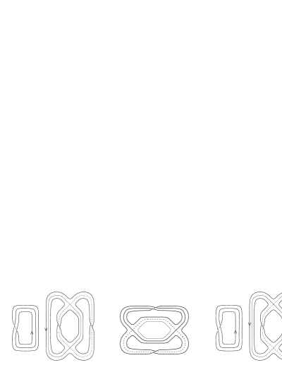
Figure 1: The simple spines $P_{1},\ldots,P_{4}$ of $M_{\Sigma_{2}}^{(1)},\ldots,M_{\Sigma_{2}}^{(4)}$. The picture always shows the boundary of a regular neighbourhood of the locus of non-surface points. To get $P_{1}$ from the two separate fragments shown one must identify the two curves marked by arrows, which constitute the core $\alpha_{1}$ of the annular 2-component of $P_{1}$, while all other 2-components are discs. The same applies to $P_{3}$, which contains an annulus with core $\alpha_{3}$. To get $P_{2}$ from the fragment shown one should attach a Möbius strip to the thick curve $\alpha_{2}$ and a disc to the other one, and the same applies to $P_{4}$, which contains a Möbius strip bounded by a curve $\alpha_{4}$.

As explained in the caption, the spines of $M_{\Sigma_{2}}^{(1)}$ and $M_{\Sigma_{2}}^{(3)}$ contain an annular 2-component, while those of $M_{\Sigma_{2}}^{(2)}$ and $M_{\Sigma_{2}}^{(4)}$ contain a Möbius strip 2-component. Let us denote by $S_{i}$ the properly embedded annulus or Möbius strip transversal to the curve $\alpha_{i}$ also described in the caption of Fig. 1.

We begin with the case $i=1,3$. As one sees from the picture, cutting $P_{i}$ along $\alpha_{i}$ one gets a disjoint union of two polyhedra that collapse respectively onto a circle and onto a graph of Euler characteristic $-1$. Since this corresponds to cutting $M_{\Sigma_{2}}^{(i)}$ along $S_{i}$, we deduce that $M_{\Sigma_{2}}^{(i)}$ is obtained by gluing a genus-2 handlebody and a solid torus along a boundary annulus. Looking at the core curves of the glued annuli, it is not difficult to show that the annulus $S_{i}$ is essential in $M_{\Sigma_{2}}^{(i)}$, so it gives the JSJ decomposition. Finally, taking a closer examination of the gluings, we saw that the annuli used in both gluings are the same, while the gluing homeomorphisms are different. This allowed us to conclude that $M_{\Sigma_{2}}^{(1)}\not\cong M_{\Sigma_{2}}^{(3)}$.

Let us now turn to the case $i=2,4$. Cutting $P_{i}$ along the core circle of the Möbius strip component (which again corresponds to cutting $M_{\Sigma_{2}}^{(i)}$ along $S_{i}$) yields a polyhedron which collapses onto a graph of Euler characteristic $-1$. Even if we get a single polyhedron, (which must be the case since this time the cut is along the core of a Möbius strip), we again conclude that the initial manifold is obtained by gluing a genus-2 handlebody and a solid torus along a boundary annulus. As before it is not hard to show that the annulus is in fact essential, so it gives the JSJ decomposition. In addition, we have proved that the annulus in the boundary of the solid torus is the same in both cases, its core being the curve of type (2,1). On the contrary, the cores of the annuli on the boundary of the genus-2 handlebody used to obtain $M_{\Sigma_{2}}^{(2)}$ and $M_{\Sigma_{2}}^{(4)}$ are those shown in Fig. 2.

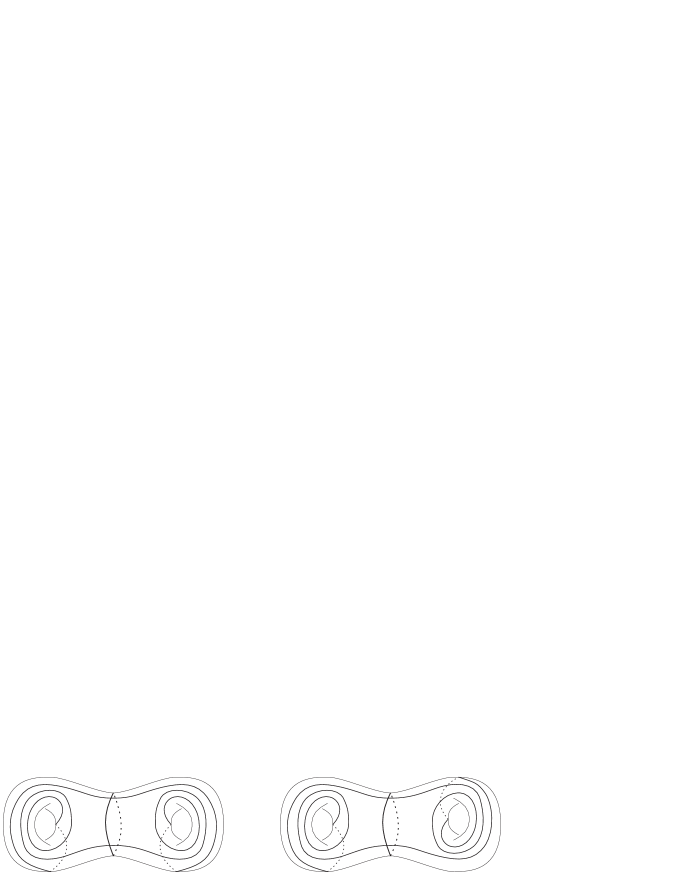
Figure 2: The core curves of the annuli used to reconstruct $M_{\Sigma_{2}}^{(2)}$ and $M_{\Sigma_{2}}^{(4)}$.

The conclusion that $M_{\Sigma_{2}}^{(2)}\not\cong M_{\Sigma_{2}}^{(4)}$ now follows from the next result, the long proof of which we only outline:

Proposition 3.6.

No homeomorphism of the genus-$2$ handlebody $H$ takes the curve $\ell_{2}$ shown in Fig. 2-left to the curve $\ell_{4}$ shown in Fig. 2-right.

Proof.

As already mentioned, we restrict ourselves to indicating the general scheme of our argument only. As one sees from Fig. 2, for $i=2,4$ there exists an essential disc $D_{i}$ in $H$ which intersects $\ell_{i}$ transversely in exactly two points. Moreover cutting $H$ along $D_{i}$ we get two solid tori $T^{0}_{i}$ and $T^{1}_{i}$ such that $\partial T^{j}_{i}$ contains a distinguished disc $\Delta^{j}_{i}$ and an arc $\beta_{i}^{j}$ properly embedded in $\partial T^{j}_{i}\setminus\Delta^{j}_{i}$. The pair $(H,\ell_{i})$ is obtained by gluing $T^{0}_{i}$ to $T^{1}_{i}$ along a homeomorphism $\Delta^{0}_{i}\to\Delta^{1}_{i}$, with $\ell_{i}$ being the image of $\beta^{0}_{i}\cup\beta^{1}_{i}$. It is actually quite easy to see that the four triples $(T^{j}_{i},\Delta^{j}_{i},\beta^{j}_{i})$ for $i=2,4$ and $j=0,1$ can be identified to each other, but after doing this the gluing homeomorphisms $\Delta^{0}_{2}\to\Delta^{1}_{2}$ and $\Delta^{0}_{4}\to\Delta^{1}_{4}$ differ by a rotation of angle $\pi$, which is isotopic to the identity but not in a way that preserves the endpoints of the arcs. The proof of the proposition then follows from the next:

Claim. For $\ell\in\{\ell_{2},\ell_{4}\}$, the disc $D$ properly embedded in $H$ which intersects $\ell$ transversely in two points and splits $H$ into two solid tori is unique up to isotopy preserving $\ell$.

The proof of this claim is rather long and technical. We consider a handle decomposition of $H$ into one 0-handle and two 1-handles. This yields a decomposition of $\partial H$ into three punctured discs, namely one sphere with four holes and two annuli. Slightly modifying the definition in [13] we then call normal with respect to this decomposition a curve in $\partial H$ which intersects each of the punctured discs along a collection of simple arcs with endpoints on different boundary components or along a simple closed curve. We next establish the following two facts:

1. Up to isotopy preserving $\ell$ there is a unique normal curve that intersects $\ell$ in two points and decomposes $H$ into two solid tori;

2. The boundary of $D$ can be isotoped (preserving $\ell$) to normal position.

This concludes our argument. ∎

Genus-2 boundary: non-hyperbolicity

To show that none of the manifolds $M_{\Sigma_{2}}^{(i)}$ is hyperbolic, we used again the idea described above. Namely, we constructed for each $M_{\Sigma_{2}}^{(i)}$ a simple spine with an annulus or Möbius strip component and we proved that the corresponding proper annulus in the manifold is essential. This was done as follows:

1. For about half of the $M_{\Sigma_{2}}^{(i)}$’s, the special spine dual to the initial triangulation already contained a 2-component incident to two vertices, so we found a simple spine with an annulus or Möbius strip 2-component by applying an inverse L-move, as above. For the other $M_{\Sigma_{2}}^{(i)}$’s we did the same but we first had to change the initial special spine, by applying first one positive $T$-move [13] and then one inverse $T$-move elsewhere.

2. From the spine of $M_{\Sigma_{2}}^{(i)}$ constructed in the previous item we got a properly embedded annulus $S_{i}$, that we then showed to be essential. We did this by cutting $M_{\Sigma_{2}}^{(i)}$ along $S_{i}$, which gave the following:

   1. In $2$ cases, a genus-2 handlebody;

   2. In $6$ cases, the union of a genus-2 handlebody and a solid torus;

   3. In $4$ cases, a manifold that could be further split along an annulus into the union of a genus-2 handlebody and a solid torus;

   4. In $4$ cases, the union of a solid torus and a manifold as described in the previous point.

   In all cases, analyzing the way $M_{\Sigma_{2}}^{(i)}$ can be reconstructed from the pieces $S_{i}$ cuts into, we could then show that it is irreducible and that within it $S_{i}$ is $\pi_{1}$-injective and not boundary-parallel, from which we got the desired conclusion.

Further information for genus-2 boundary

The decomposition (a)-(d) just described along annuli of the 16 elements of ${\mathcal{O}}^{\mathrm{non}}_{\Sigma_{2}}$ provides a rather accurate description of the topology of these manifolds. In addition to it, we mention that in cases (c) and (d) the second splitting annulus is not disjoint from the trace of $S_{i}$, so the splitting cannot be described as being along the union of two disjoint annuli.

RedTribe
Carlton, Victoria
Australia 3053
damianh@redtribe.com

Dipartimento di Matematica Applicata
Via Filippo Buonarroti, 1C
56127 PISA – Italy
petronio@dm.unipi.it

Dipartimento di Matematica Applicata
Via Filippo Buonarroti, 1C
56127 PISA – Italy
pervova@csu.ru

References

- [1] R. Benedetti – C. Petronio, “Lectures on Hyperbolic Geometry,” Springer-Verlag, Berlin-Heidelberg-New York, 1992.
- [2] P. J. Callahan – M. V. Hildebrandt – J. R. Weeks, A census of cusped hyperbolic -manifolds. With microfiche supplement, Math. Comp. 68 (1999), 321-332.
- [3] D. B. A. Epstein – R. C. Penner, Euclidean decomposition of non-compact hyperbolic manifolds, J. Differential Geom. (1) 27 (1988), 67-80.
- [4] A. T. Fomenko – S. V. Matveev, “Algorithmic and computer methods for three-manifolds,” Mathematics and its Applications, Vol. 425, Kluwer Academic Publishers, Dordrecht, 1997.
- [5] R. Frigerio – B. Martelli – C. Petronio, Small hyperbolic -manifolds with geodesic boundary, Exp. Math. 13 (2004), 171-184.
- [6] R. Frigerio – B. Martelli – C. Petronio, “Hyperbolic -manifolds with non-empty boundary,” Tables available from www.dm.unipi.it/pages/petronio/public-html.
- [7] R. Frigerio – C. Petronio, Construction and recognition of hyperbolic -manifolds with geodesic boundary, Trans. Amer. Math. Soc. 356 (2004), 3243-3282.
- [8] O. Goodman, “Snap,” The computer program for studying arithmetic invariants of hyperbolic 3-manifolds, available from http://www.ms.unimelb.edu.au/snap/ and from http://sourceforge.net/projects/snap-pari.
- [9] D. Heard, “Orb,” The computer program for finding hyperbolic structures on hyperbolic 3-orbifolds and 3-manifolds, available from http://www.ms.unimelb.edu.au/snap/orb.html.
- [10] J. Hempel, “3-Manifolds,” Ann. of Math. Studies, Vol. 86, Princeton, (1976).
- [11] S. Kojima, Polyhedral decomposition of hyperbolic manifolds with boundary, Proc. Work. Pure Math. 10 (1990), 37-57.
- [12] S. Kojima, Polyhedral decomposition of hyperbolic -manifolds with totally geodesic boundary, In: “Aspects of Low-Dimensional Manifolds,” Adv. Stud. Pure Math. Vol. 20, Kinokuniya, Tokyo, 1992, 93-112.
- [13] S. V. Matveev, “Algorithmic Topology and Classification of -Manifolds,” ACM-monographs Vol. 9, Springer-Verlag, Berlin-Heidelberg-New York, 2003.
- [14] S. V. Matveev – V. V. Tarkaev, “Three-manifold Recognizer”, A computer program for recognition of 3-manifolds, available from http://www.csu.ac.ru/trk/spine/.
- [15] G. Perelman, The entropy formula for the Ricci flow and its geometric applications, preprint math.DG/0211159.
- [16] G. Perelman, Ricci flow with surgery on three-manifolds, preprint math.DG/0303109.
- [17] G. Perelman, Finite extinction time for the solutions to the Ricci flow on certain three-manifolds, preprint math.DG/0307245.
- [18] J. G. Ratcliffe, “Foundations of Hyperbolic Manifolds,” Second Edition, Graduate Texts in Math. Vol. 149, Springer-Verlag, New York, 2006.
- [19] C. P. Rourke – B. J. Sanderson, “Introduction to Piecewise-Linear Topology,” Ergebn. der Math. Vol. 69, Springer-Verlag, New York-Heidelberg, 1972.
- [20] M. Sakuma – J. R. Weeks, The generalized tilt formula, Geom. Dedicata 50 (1995), 1-9.
- [21] W. P. Thurston, “The Geometry and Topology of -manifolds,” mimeographed notes, Princeton, 1979.
- [22] V. G. Turaev – O. Ya. Viro, State sum invariants of -manifolds and quantum -symbols, Topology (4) 31 (1992), 865-902.
- [23] A. Ushijima, The tilt formula for generalized simplices in hyperbolic space, Discrete Comput. Geom. 28 (2002), 19-27.
- [24] A. Ushijima, A volume formula for generalised hyperbolic tetrahedra, In: “Non-Euclidean Geometries”, Mathematics and Its Applications, Vol. 581, Springer, NY, 2006, 249-265.
- [25] J. R. Weeks, “SnapPea”, The hyperbolic structures computer program, available from www.geometrygames.org.