On the influence of time and space correlations on the next earthquake magnitude

Abstract

A crucial point in the debate on feasibility of earthquake prediction is the dependence of an earthquake magnitude from past seismicity. Indeed, whilst clustering in time and space is widely accepted, much more questionable is the existence of magnitude correlations. The standard approach generally assumes that magnitudes are independent and therefore in principle unpredictable. Here we show the existence of clustering in magnitude: earthquakes occur with higher probability close in time, space and magnitude to previous events. More precisely, the next earthquake tends to have a magnitude similar but smaller than the previous one. A dynamical scaling relation between magnitude, time and space distances reproduces the complex pattern of magnitude, spatial and temporal correlations observed in experimental seismic catalogs.

Since the Omori observation omori , temporal clustering is considered a general and distinct feature of seismic occurrence. Clustering in space has also been well established kagknop and, together with the Omori law and the Gutenberg-Richter law GR , is the main ingredient of probabilistic tools for time-dependent seismic hazard evaluation reajon ; ogata ; gerg . The distribution $D(\Delta t)$ of the inter-time $\Delta t$ elapsed between two successive events is a suitable quantity to characterize the temporal organization of seismicity. Analogously, the distribution $D(\Delta r)$ of the distance $\Delta r$ between subsequent epicenters provides useful insights in the spatial organization. Both distributions have been the subject of much interest in the last years bak ; mega ; yang ; corral ; corral1 ; scaf ; lind ; livina ; noisoc ; sorn2 ; davpac ; corral2 ; corral3 ; noi . In particular, they exhibit universal behavior essentially independent of the space region and the magnitude range considered corral ; sorn2 ; davpac ; corral3 . Furthermore, the question of the existence of correlations between magnitudes of subsequent earthquakes has been also recently addressed noi ; corral1 ; corral2 . In ref.corral1 ; corral2 , Corral has shown that the Southern California Catalog exhibits possible magnitude correlations that are small but different from zero. However, restricting his investigation to earthquakes with $\Delta t$ greater then $30$ minutes, he observes that correlations reduce and become smaller than statistical uncertainty. Magnitude correlations have been, therefore, interpreted as a spurious effect due to short term aftershock incompleteness (STAI) kagan . According to this hypothesis, aftershocks, in particular small events, occurring closely after large shocks are not reported in the experimental catalog. This interpretation agrees with the standard approach that assumes independence of earthquake magnitudes: an earthquake ”does not know how large it will become”. This has strong implications on the still open question of earthquake predictability nat . On the other hand, a recent analysis of the Southern California Catalog noi has shown the existence of non-zero magnitude correlations, not to be attributed to STAI. These are observed by means of an averaging procedure that reduces statistical fluctuations. A dynamical scaling hypothesis relating magnitude to time differences has been proposed to explain the observed magnitude correlations.

In this paper we present a statistical analysis of experimental catalogs that confirms the existence of relevant magnitude correlations. In particular, the analysis enlightens the structure of these correlations and their relationship with $\Delta t$ and $\Delta r$. We then introduce a trigger model based on a dynamical scaling relation between energy, space and time and show that this model reproduces the above experimental findings. We consider the NCEDC catalog (downloaded at http:///www.ncedc.org/ncedc/, years 1974-2002, South (North) lat. 32 (37), West (East) long. -122 (-114)). Similar results are obtained for seismic catalogs of other geographic regions. To ensure catalog completeness, we consider only events with magnitudes $m\geq 3$ and take into account STAI using the method proposed in ref.helmkag . The quantities considered are $\Delta t_{i}=t_{i+1}-t_{i}$, $\Delta r_{i}=|\vec{r}_{i+1}-\vec{r}_{i}|$ and $\Delta m_{i}=m_{i+1}-m_{i}$, i.e. the time, space and magnitude difference between subsequent events. We have also evaluated the quantity $\Delta m^{*}_{i}=m_{i^{*}}-m_{i}$ where $i^{*}\neq i$ is the random index of an earthquake recorded in the catalog. Hence, $\Delta m_{i}^{*}$ is the magnitude difference within a reshuffled catalog where the magnitude of the subsequent earthquake is independent of previous ones. We then consider the conditional probability

$$P(\Delta x_{i}<x_{0}|\Delta y_{i}<y_{0})\equiv\frac{N(x_{0},y_{0})}{N(y_{0})}$$ (1)

where $N(x_{0},y_{0})$ is the number of couples of subsequent events with both $\Delta x_{i}<x_{0}$ and $\Delta y_{i}<y_{0}$ and $N(y_{0})$ is the number of couples with $\Delta y_{i}<y_{0}$. In the following $\Delta x_{i}$ or $\Delta y_{i}$ will be used to indicate, depending on cases, $\Delta r_{i}$, $\Delta t_{i}$, $\Delta m_{i}$ or $\Delta m_{i}^{*}$. Our method is schematically presented in Fig.1. Keeping $m_{0}$ and $r_{0}$ fixed, we compute the quantity $P(\Delta m^{*}_{i}<m_{0}|\Delta r_{i}<r_{0})$ for several independent random realizations of the reshuffled catalog, obtaining the distribution $\rho\left[P(\Delta m^{*}_{i}<m_{0}|\Delta r_{i}<r_{0})\right]$. Taking $10^{4}$ independent realizations of the magnitude reshuffling, for each given $m_{0}$ and $r_{0}$, we always find that $\rho\left[P(\Delta m^{*}_{i}<m_{0}|\Delta r_{i}<r_{0})\right]$ is gaussian distributed with mean value $Q(m_{0},r_{0})$ and standard deviation $\sigma(m_{0},r_{0})$. Analogous behaviour is obtained for $P(\Delta m^{*}_{i}<m_{0}|\Delta t_{i}<t_{0})$ and we similarly define $Q(m_{0},t_{0})$ and $\sigma(m_{0},t_{0})$. The relevant quantity is $\delta P(m_{0},y_{0})=P(\Delta m_{i}<m_{0}|\Delta y_{i}<y_{0})-Q(m_{0},y_{0})$, i.e the difference between the value of $P(\Delta m_{i}<m_{0}|\Delta y_{i}<y_{0})$ in the real catalog and its mean value in the reshuffled one. If the absolute value $|\delta P(m_{0},y_{0})|$ is larger than $\sigma(m_{0},y_{0})$, significant non-zero correlations between magnitudes of successive earthquakes exist. In particular, a positive value of $\delta P(m_{0},y_{0})>\sigma(m_{0},y_{0})$ implies that the number of couples $N(m_{0},y_{0})$ is significantly larger in the real catalog with respect to a catalog where magnitudes are uncorrelated. In Fig.1 we explicitly compare $\rho\left[P(\Delta m^{*}_{i}<m_{0}|\Delta y_{i}<y_{0})\right]$ with $P(\Delta m_{i}<m_{0}|\Delta y_{i}<y_{0})$ for $m_{0}=0$ and $y_{0}=r_{0}=10km$ or $y_{0}=t_{0}=1h$. One clearly observes the existence of non-zero magnitude correlations, since $\delta P(m_{0},r_{0})\simeq 8.3\sigma(m_{0},r_{0})$ and $\delta P(m_{0},t_{0})\simeq 7.3\sigma(m_{0},t_{0})$. For a deeper understanding of the nature of the observed correlations, the above analysis has been extended to other values of $m_{0}$, $r_{0}$ and $t_{0}$. In Fig.2 and Fig.3 we plot the quantities $\delta P(m_{0},r_{0})$ and $\delta P(m_{0},t_{0})$ as a function of $m_{0}$ for different values of $r_{0}$ and $t_{0}$ respectively. The error bar of each point is the standard deviation $\sigma(m_{0},y_{0})$. We first observe that for each value of $r_{0}$ and $t_{0}$ and for a wide range of $m_{0}$, $\delta P(m_{0},y_{0})$ is strictly positive and significantly different from zero. Considering the behavior at fixed $r_{0}$ or $t_{0}$, the curve has a peak centered in $m_{0}\lesssim 0$, indicating a crossover from positive to negative correlations. This can be better enlightened by the derivative $P^{\prime}(m_{0},y_{0})=\frac{d\delta P(m_{0},y_{0})}{dm_{0}}=$, which represents the probability difference for $\Delta m_{i}=m_{0}$ conditioned to $\Delta y_{i}<y_{0}$ . $P^{\prime}(m_{0},y_{0})$ is therefore an estimate of the magnitude correlation between two subsequent events with $\Delta m_{i}=m_{0}$. Interestingly, for both $y_{0}=r_{0}$ and $y_{0}=t_{0}$ (inset of Fig.2 and Fig.3), $P^{\prime}(m_{0},y_{0})$ has the maximum value for $m_{0}$ in the range $[-1,-0.5]$ and decreases to zero for smaller values of $m_{0}$. For $m_{0}\geq 0$, $P^{\prime}(m_{0},y_{0})$ is always negative with the minimum value centered around $m_{0}\in[0,0.5]$ and going to zero for large $m_{0}$. This implies that, for positive $m_{0}$, the probability is larger in a reshuffled catalog than in the real one. As a consequence, Fig.s (2,3) clearly show that the magnitudes of subsequent earthquakes are correlated and, in particular, the next earthquake tends to have a magnitude close but smaller than the previous one. Furthermore, Fig.s (2,3) indicate that for any fixed $m_{0}$, curves corresponding to different $r_{0}$ or $t_{0}$ clearly separate, showing the existence of correlations between $\Delta m$ and $\Delta r$, $\Delta m$ and $\Delta t$. In particular we observe that the larger are $r_{0}$ or $t_{0}$, the smaller are magnitude correlations.

To better investigate the role of $r_{0}$ and $t_{0}$ on magnitude correlations, we consider $P(\Delta r_{i}<r_{0}|\Delta m_{i}<m_{0})$ and $P(\Delta t_{i}<t_{0}|\Delta m_{i}<m_{0})$. Following the procedure described for Fig.1, we compute $\delta P(x_{0},m_{0})$ and $\sigma(x_{0},m_{0})$ for $x_{0}=r_{0},t_{0}$ (Fig.4). Also in this case, a non-zero $\delta P(x_{0},m_{0})$ is the signature of magnitude correlations. We observe that, for each value of $m_{0}$, $\delta P(x_{0},m_{0})$ is a decreasing function of $r_{0}$ and $t_{0}$ and therefore stronger correlations are observed for events that occur closely in time and space. More specifically, Fig.4 shows that for smaller values of $t_{0}$ and $r_{0}$, the probability to have $\Delta m_{i}\leq-2$ is about $40\%$ larger in the real than in a given reshuffled catalog.

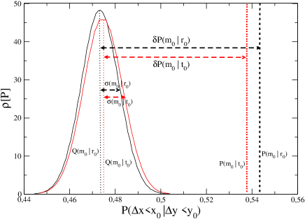
Figure 1: (Color online) The distribution of $P(\Delta m^{*}_{i}<m_{0}|\Delta r_{i}<r_{0})$ for $r_{0}=10Km$ and $m_{0}=0$ (black curve) is compared with $P(\Delta m_{i}<0|\Delta r_{i}<10Km)=0.543$ (broken black curve). $\rho[P]$ has a gaussian behaviour with mean $Q(m_{0},r_{0})=0.473$ and standard deviation $\sigma(m_{0},r_{0})=0.00825$. For $r_{0}=10Km$ and $m_{0}=0$ one has $\delta P(m_{0},r_{0})=0.07\simeq 8.5\sigma(m_{0},r_{0})$ strongly supporting the existence of correlations between $m_{i}$ and $m_{i-1}$. The same conclusion can be obtained by considering $P(\Delta m^{*}_{i}<m_{0}|\Delta t_{i}<t_{0})$ for $t_{0}=1h$ and $m_{0}=0$ (red curve). It is found $P(\Delta m_{i}<0|\Delta t_{i}<1h)=0.537$ (broken red curve) whereas $\rho[P]$ is a gaussian with mean $Q(m_{0},t_{0})=0.475$ and standard deviation $\sigma(m_{0},t_{0})=0.0085$. As a consequence $\delta P(m_{0},t_{0})\simeq 7.3\sigma(m_{0},t_{0})$.

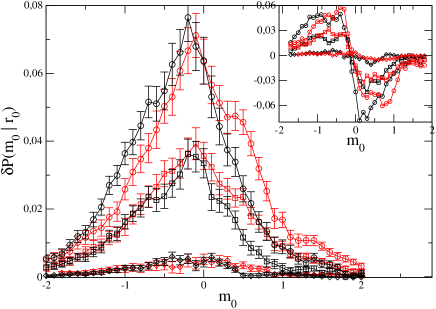
Figure 2: (Color online) The quantity $\delta P(m_{0},r_{0})$ as a function of $m_{0}$ for $r_{0}=10,100,500Km$ from top to bottom. For each $r_{0}$ and $m_{0}$ the error bar is the standard deviation $\sigma(m_{0},r_{0})$. Data for the Southern California catalog (black) are compared with numerical simulations (red). In the inset, the quantity $P^{\prime}(m_{0},r_{0})$.

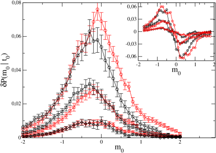
Figure 3: (Color online) The quantity $\delta P(m_{0},t_{0})$ as a function of $m_{0}$ for $t_{0}=1,10,50hours$ from top to bottom. For each $t_{0}$ and $m_{0}$ the error bar is the standard deviation $\sigma(m_{0},t_{0})$. Data for the Southern California catalog (black) are compared with numerical simulations (red). In the inset, the quantity $P^{\prime}(m_{0},t_{0})$.

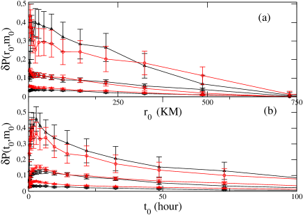
Figure 4: (Color online) (a) The quantity $\delta P(r_{0},m_{0})$ as a function of $r_{0}$ for $m_{0}=2,0.5,0$ from top to bottom. (b) The quantity $\delta P(t_{0},m_{0})$ as a function of $r_{0}$ for $m_{0}=2,0.5,0$ from top to bottom. Data for the experimental catalog (black) are compared with numerical simulations (red). For each point the error bar is the standard deviation $\sigma(x_{0},m_{0})$.

The above analysis shows that a better description of real seismicity can be obtained if correlations between time, space and magnitude are properly taken into account. As in dynamical critical phenomena where energy and time fix a characteristic length scale, similar ideas can be used to introduce magnitude correlations within standard trigger models for seismicity. In trigger models vere-jones , the probability to have the next earthquake in the time window $[t,t+\delta t]$, with epicenter in the region $[\vec{r},\vec{r}+\delta\vec{r}]$ and magnitude in the range $[m,m+\delta m]$ is given by the superposition

$${\cal P}(t,\vec{r},m)=\sum_{j}P(t-t_{j},|\vec{r}-\vec{r}_{j}|,m,m_{j}),$$ (2)

where $P(t-t_{j},|\vec{r}-\vec{r}_{j}|,m,m_{j})$ is the probability conditioned to the occurrence of an earthquake of magnitude $m_{j}$, at time $t_{j}<t$, in the position $\vec{r}_{j}$ . In the widely accepted ETAS model ogata , $m,m_{j},t-t_{j}$ and $|\vec{r}-\vec{r}_{j}|$ are all independent quantities and empirical laws are used to characterize their distributions. Many analytical and numerical studies show that the ETAS model captures several aspects of real seismic occurrence ogata ; ogata2 ; helmstetter ; etas ; sorn2 ; saichev1 . Nevertheless, because of the assumption of independence between $m$ and $m_{j}$, $\delta P(x,y)$ would be a random fluctuating function with zero average and standard deviation $\sigma(x,y)$, in all cases considered in Fig.s (2-4). Hence, by construction, the ETAS model does not take into account magnitude correlations and their dependence on time and space.

In order to reproduce the experimental findings, we introduce

$$\tau_{ij}=k_{t}10^{b(m_{i}-m_{j})}\hskip 14.22636pt{\rm and}\hskip 14.22636ptr_{ij}^{z}=k_{r}|\vec{r}_{i}-\vec{r}_{j}|^{z}$$ (3)

which fix two characteristic time scales leading to the scaling behaviour with $\Delta t_{ij}=t_{i}-t_{j}$

$$P(\Delta t_{ij},|\vec{r}_{i}-\vec{r}_{j}|,m_{i},m_{j})=\Delta t_{ij}^{-2/z}H\left(\frac{\tau_{ij}}{\Delta t_{ij}},\frac{r_{ij}}{\Delta t_{ij}^{1/z}}\right).$$ (4)

The exponent $2/z$ is determined by imposing the condition $\int d\vec{r}_{i}P(\Delta t_{ij},|\vec{r}_{i}-\vec{r}_{j}|,m_{i},m_{j})=H_{1}\left(\frac{\tau_{ij}}{\Delta t_{ij}}\right)$, where the function $H_{1}(x)$ must satisfy the normalization condition $\int dxH_{1}(x)=1$. Following ref. noi it is possible to show that this normalization removes the problem with “ultaviolet” and “infrared” divergences of the ETAS model saichev1 .

In order to simplify the numerical procedure, we consider a special case of Eq.(4)

$$H\left(\frac{\tau_{ij}}{\Delta t_{ij}},\frac{r_{ij}}{\Delta t_{ij}^{1/z}}\right)=H_{1}\left(\frac{\tau_{ij}}{\Delta t_{ij}}\right)H_{2}\left(\frac{r_{ij}}{\Delta t_{ij}^{1/z}}\right).$$ (5)

In the numerical simulation, we generate a synthetic catalog containing only occurrence times and magnitudes. We start with a random event at initial time $t_{0}=0$, time is then increased by one unit and a trial magnitude is randomly chosen. The $i$-th event, at time $t_{i}$ and with magnitude $m_{i}$, occurs with a probability $\sum_{j<i}H_{1}(\tau_{ij}/\Delta t_{ij})$ where the sum is over all previous events. In particular we use

$$H_{1}(x)=\frac{A}{e^{x}-1+\gamma_{1}}$$ (6)

with the parameters $k_{t}=12.7h$, $A=0.21h^{-1}$, $\gamma_{1}=0.1$ and $b=0.9$, that in ref.noi are found able to reproduce the experimental behavior of magnitude and inter-time distributions. To introduce the epicenter location in the numerical catalog we use the power law

$$H_{2}(x)=\frac{B}{x^{\mu}+\gamma_{2}}$$ (7)

where $\mu$ and $\gamma_{2}$ are fit-parameters and $B$ is fixed by the normalization. Other functional forms for $H_{2}(x)$ give similar results but with a worse agreement with experimental data. We follow the method used in ref.helmstetter ; ogata2 for the ETAS model. More precisely, for $j=0$ the epicenter of the first event in the catalog $\vec{r}_{j=0}$ is randomly fixed in a point of a square lattice of size $L$. For sufficiently large lattices, the results are $L$ independent. Next, $j$ is updated $j=j+1$, and the mother of the $j-th$ earthquake is chosen among all previous $0\leq i\leq j-1$ events according to the probability $H_{1}\left(\frac{\tau_{ij}}{\Delta t_{ij}}\right)$. Once the mother event is identified, its epicenter $\vec{r}^{*}$ and occurrence time $t^{*}$ are used to randomly obtain $\vec{r}_{j}$ from the probability distribution $(t_{j}-t^{*})^{-2/z}H_{2}\left(\frac{|\vec{r}_{j}-\vec{r}^{*}|}{(t_{j}-t^{*})^{1/z}}\right)$ and assuming space isotropy.

The numerical catalog is analyzed with the same procedure applied to experimental data. Numerical results for $\delta P(x_{0},y_{0})$ are presented as red circles in Fig.s (2-4) for $\mu=2.6$, $k_{r}=0.03h/Km^{z}$, $z=3.3$ and $\gamma_{2}=0.1$. We observe a very good agreement between numerical and experimental data. In particular, $\delta P(m_{0},y_{0})$ (Fig.s(2,3)) displays a maximum value localized around the maximum of the experimental distribution. Furthermore, also the functional form of the decay of $\delta P(x_{0},m_{0})$ for both $x_{0}=r_{0}$ (Fig.4a) and $x_{0}=t_{0}$ (Fig.4b) is reproduced.

The agreement between numerical and experimental results, indicates that the scaling relation (4) among magnitudes, times, and epicenter distances can describe the complex pattern of the experimentally observed correlations. The origin of magnitude correlations, within our theoretical approach, has a direct interpretation. According to Eq.s (5,6,7), indeed, at the time $t$ an earthquake of magnitude $m$ with epicenter $\vec{r}$ has a finite probability to be triggered by a previous ($m_{j},t_{j},\vec{r}_{j}$) earthquake only if $m<m_{j}-(1/b)\log((t-t_{j})/k_{t})$ and $r_{ij}<(t-t_{j})^{1/z}$ (Eq. (3)). As a consequence, only events occurring close in time and space can have a magnitude close and smaller, or even larger, that the previous triggering one. Magnitude correlations, therefore, become particularly relevant within aftershock sequences, when earthquakes tend to be very close in time and space. Thus a dynamical scaling approach, that properly takes into account these correlations, can improve existing methods for time dependent hazard evaluation.

References

- (1) F. Omori, J. Coll. Sci. Imp. Univ. Tokyo 7, 111, (1894)
- (2) Y.Y. Kagan, L. Knopoff, Geophys. J. Roy. Astron. Soc. 62, 303 (1980)
- (3) B. Gutenberg, C.F. Richter, Bull. Seism. Soc. Am. 34, 185 (1944)
- (4) Y. Ogata, J. Amer. Stat. Assoc. 83, 9, (1988)
- (5) P.A Reasenberg, L.M. Jones, Science 243, 1173 (1989)
- (6) M.C. Gerstenberger, S. Wiemer, L.M. Jones, P.A. Reasenberg, Nature 435, 328 (2005)
- (7) P. Bak, K. Christensen, L. Danon, T. Scanlon, Phys. Rev. Lett. 88, 178501, (2002)
- (8) M.S. Mega et al., Phys. Rev. Lett. 90, 188501 (2003)
- (9) A. Corral, Phys. Rev. Lett. 92, 108501 (2004)
- (10) X. Yang, S. Du, J. Ma, Phys. Rev. Lett. 92, 228501 (2004)
- (11) N. Scafetta, B.J. West Phys. Rev. Lett. 92, 138501 (2004).
- (12) M. Lindman, K. Jonsdottir, R. Roberts, B. Lund, R. Bodvarsson, Phys. Rev. Lett. 94, 108501 (2005)
- (13) V. N. Livina, S. Havlin, A. Bunde Phys. Rev. Lett. 95, 208501 (2005)
- (14) E. Lippiello, C. Godano, L. de Arcangelis, Europhys. Lett. 72, 678 (2005)
- (15) A. Saichev, D. Sornette, Phys. Rev. Lett. 97, 078501 (2006).
- (16) J. Davidsen, M. Paczuski, Phys. Rev. Lett. 94, 048501 (2005).
- (17) A. Corral, Phys. Rev. Lett. 97, 178501 (2006)
- (18) A. Corral, Phys. Rev. Lett. 95, 159801 (2005)
- (19) A. Corral, TectonoPhysics 424, 177 (2006)
- (20) E. Lippiello, C. Godano, L. de Arcangelis, Phys. Rev. Lett. 98, 098501 (2007)
- (21) Y.Y. Kagan, Bull. Seism. Soc. Amer., 94(4), 1207 (2004)
- (22) http://www.nature.com/nature/debates/earthquake/ index.html
- (23) A. Helmstetter, Y. Kagan, D. Jackson, J. Geophys. Res. 110, B05S08 (2005)
- (24) J. F. D. Vere-Jones, J. Roy. Statist. Soc., B32, 1, (1970)
- (25) Y. Ogata, Ann. Inst. Stat. Math 50, 379, (1998)
- (26) A. Helmstetter, D. Sornette, Phys. Rev. E 66 061104 1, (2002);
- (27) A. Helmstetter, D. Sornette, J. Geophys. Res. 107 2237, (2002); A. Saichev, D. Sornette Phys. Rev. E, 70, 046123 (2004); A. Saichev, A. Helmstetter, D. Sornette, Pure and Applied Geophysics, 162, 1113, (2005); D. Sornette, M.J. Werner J. Geophys. Res., 110, B09303, (2005)
- (28) A. Saichev, D. Sornette, Phys. Rev. E 72, 056122 (2005)