Overlap-free words and spectra of matrices

Abstract

Overlap-free words are words over the binary alphabet $A=\{a,b\}$ that do not contain factors of the form $xvxvx$, where $x\in A$ and $v\in A^{*}$. We analyze the asymptotic growth of the number $u_{n}$ of overlap-free words of length $n$ as $\,n\to\infty$. We obtain explicit formulas for the minimal and maximal rates of growth of $u_{n}$ in terms of spectral characteristics (the lower spectral radius and the joint spectral radius) of certain sets of matrices of dimension $20\times 20$. Using these descriptions we provide new estimates of the rates of growth that are within $0.4\%$ and $0.03\%$ of their exact values. The best previously known bounds were within $11\%$ and $3\%$ respectively. We then prove that the value of $u_{n}$ actually has the same rate of growth for “almost all” natural numbers $n$. This “average” growth is distinct from the maximal and minimal rates and can also be expressed in terms of a spectral quantity (the Lyapunov exponent). We use this expression to estimate it. In order to obtain our estimates, we introduce new algorithms to compute spectral characteristics of sets of matrices. These algorithms can be used in other contexts and are of independent interest.

1 Introduction

Binary overlap-free words have been studied for more than a century. These are words over the binary alphabet $A=\{a,b\}$ that do not contain factors of the form $xvxvx,$ where $x\in A$ and $v\in A^{*}.$ For instance, the word baabaa is overlap free, but the word baabaab is not, since it can be written $xuxux$ with $x=b$ and $u=aa.$ See [1] for a recent survey. Thue [22, 23] proved in 1906 that there are infinitely many overlap-free words. Indeed, the well-known Thue-Morse sequence is overlap-free, and so the set of its factors provides an infinite number of different overlap-free words. The asymptotics of the number $u_{n}$ of such words of a given length $n$ was analyzed in a number of subsequent contributions. The number of factors of length $n$ in the Thue-Morse sequence is proved in [6] to be larger than $3n$, thus providing a linear lower bound on $u_{n}$:

$$u_{n}\ \geq\ 3\,n.$$

The next improvement was obtained by Restivo and Salemi [20]. By using a certain decomposition result, they showed that the number of overlap-free words grows at most polynomially:

$$u_{n}\ \leq\ C\,n^{\,r},$$

where $r=\log(15)\approx 3.906.$ This bound has been sharpened successively by Kfoury [11], Kobayashi [12], and finally by Lepisto [13] to the value $r=1.37$. One could then suspect that the sequence $u_{n}$ grows linearly. However, Kobayashi [12] proved that this is not the case. By enumerating the subset of overlap-free words of length $n$ that can be infinitely extended to the right he showed that $u_{n}\ \geq\ C\,n^{\,1.155}$ and so we have

$$C_{1}\,n^{\,1.155}\leq u_{n}\leq C_{2}\,n^{\,1.37}.$$

It is worth noting that the sequence $u_{n}$ is $2$-regular, as shown by Carpi [7]. On Figure 1(a) we show the values of the sequence $u_{n}$ for $1\leq n\leq 200$ and on Figure 1(b) we show the behavior of $\log{u_{n}}/\log{n}$ for larger values of $n$. One can see that the sequence $u_{n}$ is not monotonic, but is globally increasing with $n$. Moreover the sequence does not appear to have a polynomial growth since the value $\log{u_{n}}/\log{n}$ does not seem to converge. In view of this, a natural question arises: is the sequence $u_{n}$ asymptotically equivalent to $n^{r}$ for some $r$ ? Cassaigne proved in [8] that the answer is negative. He introduced the lower and the upper exponents of growth:

$$\alpha = \sup\bigl{\{}r\ \bigl{|}\exists C>0,u_{n}\geq Cn^{r}\bigr{\}},$$ (1)

$$\beta = \inf\bigl{\{}r\ \bigl{|}\exists C>0,u_{n}\leq Cn^{r}\bigr{\}},$$

and showed that $\,\alpha<\beta$. Cassaigne made a real breakthrough in the study of overlap-free words by characterizing in a constructive way the whole set of overlap-free words. By improving the decomposition theorem of Restivo and Salemi he showed that the numbers $u_{n}$ can be computed as sums of variables that are obtained by certain linear recurrence relations. These relations are explicitly given in the next section and all numerical values can be found in Appendix A. As a result of this description, the number of overlap-free words of length $n$ can be computed in logarithmic time. For the exponents of growth Cassaigne has also obtained the following bounds: $\alpha<1.276$ and $\beta>1.332.$ Thus, combining this with the earlier results described above, one has the following inequalities:

$$1.155\ <\ \alpha\ <\ 1.276\qquad\mbox{and}\qquad 1.332\ <\ \beta\ <\ 1.37.$$ (2)

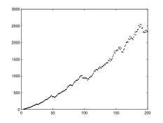
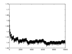
(a)	(b)

Figure 1: The values of $u_{n}$ for $1\leq n\leq 200$ (a) and $\log{u_{n}}/\log{n}$ for $1\leq n\leq 10000$ (b).

In this paper we develop a linear algebraic approach to study the asymptotic behavior of the number of overlap-free words of length $n$. Using the results of Cassaigne we show in Theorem 2 that $u_{n}$ is asymptotically equivalent to the norm of a long product of two particular matrices $A_{0}$ and $A_{1}$ of dimension $20\times 20$. This product corresponds to the binary expansion of the number $n-1$. Using this result we express the values of $\alpha$ and $\beta$ by means of certain joint spectral characteristics of these matrices. We prove that $\,\alpha\,=\,\log_{2}\check{\rho}(A_{0},A_{1})\,$ and $\,\beta\,=\,\log_{2}{\hat{\rho}}(A_{0},A_{1})$, where ${\check{\rho}}$ and ${\hat{\rho}}$ denote, respectively, the lower spectral radius and the joint spectral radius of the matrices $A_{0},A_{1}$ (we define these notions in the next section). In Section 3, we estimate these values and we obtain the following improved bounds for $\alpha$ and $\beta$:

$$1.2690\ <\ \alpha\ <\ 1.2736\qquad\mbox{and}\qquad 1.3322\ <\ \beta\ <\ 1.3326.$$ (3)

Our estimates are, respectively, within $0.4\%$ and $0.03\%$ of the exact values. In addition, we show in Theorem 3 that the smallest and the largest rates of growth of $u_{n}$ are effectively attained, and there exist positive constants $C_{1},C_{2}$ such that $\ C_{1}\,n^{\alpha}\ \leq\ u_{n}\ \leq\ C_{2}\,n^{\,\beta}$ for all $n\in{\mathbb{N}}$.

Although the sequence $\,u_{n}\,$ does not exhibit an asymptotic polynomial growth, we then show in Theorem 5 that for “almost all” values of $n$ the rate of growth is actually equal to  $\,\sigma\,=\,\log_{2}\,\bar{\rho}(A_{0},A_{1})$, where $\bar{\rho}$ is the Lyapunov exponent of the matrices. For almost all values of $n$ the number of overlap-free words does not grow as $n^{\alpha}$, nor as $n^{\beta}$, but in an intermediary way, as $n^{\sigma}$. This means in particular that the value $\frac{\,\log\,u_{n}}{\log\,n}\,$ converges to $\sigma$ as $\,n\to\infty$ along a subset of density $1$. We obtain the following bounds for the limit $\sigma,$ which provides an estimation within $0.8\%$ of the exact value:

$$1.3005<\sigma<1.3098.$$

These bounds clearly show that $\,\alpha<\sigma<\beta$.

To compute the exponents $\alpha$ and $\sigma$ we introduce new efficient algorithms for estimating the lower spectral radius $\check{\rho}$ and the Lyapunov exponent $\bar{\rho}$ of matrices. These algorithms are both of independent interest as they can be applied to arbitrary matrices.

Our linear algebraic approach not only allows us to improve the estimates of the asymptotics of the number of overlap-free words, but also clarifies some aspects of the nature of these words. For instance, we show that the “non purely overlap-free words” used in [8] to compute $u_{n}$ are asymptotically negligible when considering the total number of overlap-free words.

The paper is organized as follows. In the next section we formulate and prove the main theorems (except for Theorem 2, whose proof is quite technical and is given in Appendix B). Then in Section 3 we present algorithms for estimating the joint spectral radius, the lower spectral radius, and the Lyapunov exponent of linear operators. Applying them to those special matrices we obtain the estimations for $\,\alpha,\beta$ and $\sigma$. In the appendices we write explicit forms of the matrices and initial vectors used to compute $u_{n}$, we give a proof of Theorem 2 and present the results of our numerical algorithms.

2 The asymptotics of the overlap-free words

In the sequel we use the following notation: ${\mathbb{R}}^{d}$ is the $d$-dimensional space, inequalities $x\geq 0$ and $A\geq 0$ mean that all the entries of the vector $x$ (respectively, of the matrix $A$) are nonnegative. We denote ${\mathbb{R}}^{d}_{+}=\{x\in{\mathbb{R}}^{d},\ x\geq 0\}$, by $|x|$ we denote a norm of the vector $x\in{\mathbb{R}}^{d}$, and by $\|\cdot\|$ any matrix norm. In particular, $|x|_{1}=\sum\limits_{i=1}^{d}|x_{i}|,\ \|A\|_{1}=\sup_{|x|_{1}=1}|Ax|=\max_{j=1,\ldots d}\sum_{i=1}^{d}|A_{ij}|$. We write ${\bf 1}$ for the vector $(1,\ldots,1)^{T}\in{\mathbb{R}}^{d}$, $\rho(A)$ for the spectral radius of the matrix $A$, that is, the largest magnitude of its eigenvalues. If $A\geq 0$, then there is a vector $v\geq 0$ such that $Av=\rho(A)v$ (the so-called Perron-Frobenius eigenvector). For two functions $f_{1},f_{2}$ from a set $Y$ to ${\mathbb{R}}_{+}$ the relation $f_{1}(y)\asymp f_{2}(y)$ means that there are positive constants $C_{1},C_{2}$ such that $C_{1}f_{1}(y)\leq f_{2}(y)\leq C_{2}f_{1}(y)$ for all $y\in Y$.
To compute the number $u_{n}$ of overlap-free words of length $n$ we use several results from [8] that we summarize in the following theorem:

Theorem 1

Let $F_{0},F_{1}\in{\mathbb{R}}^{30\times 30},$ and let $w,y_{3},\dots,y_{15}\in{\mathbb{R}}_{+}^{30}$ be as given in Appendix A. For $n\geq 16$, let $y_{n}$ be the solution of the following recurrence equations

$$\begin{array}[]{ccc}y_{2n}&=&F_{0}y_{n}\\ y_{2n+1}&=&F_{1}y_{n}.\end{array}$$ (4)

Then, for any $n\geq 16,$ the number of overlap-free words of length $n$ is equal to $w^{T}y_{n-1}.$

It follows from this result that the number $u_{n}$ of overlap-free words of length $n\geq 16$ can be obtained by first computing the binary expansion $d_{k}\cdots d_{1}$ of $n-1$, i.e., $n-1=\sum_{j=0}^{k-1}d_{j+1}2^{j}$, and then defining

$$u_{n}=w^{T}F_{d_{1}}\cdots F_{d_{k-4}}y_{m}$$ (5)

where $m=d_{k-3}+d_{k-2}2+d_{k-1}2^{2}+d_{k}2^{3}$. To arrive at the results summarized in Theorem 1, Cassaigne builds a system of recurrence equations allowing the computation of a vector $U_{n}$ whose entries are the number of overlap-free words of certain types (there are $16$ different types). These recurrence equations also involve the recursive computation of a vector $V_{n}$ that counts other words of length $n,$ the so-called “single overlaps”. The single overlap words are not overlap-free, but have to be computed, as they generate overlap-free words of larger lengths. We now present the main result of this section which improves the above theorem in two directions. First we reduce the dimension of the matrices from 30 to 20, and second we prove that $u_{n}$ is given asymptotically by the norm of a matrix product. The reduction of the dimension to 20 has a straightforward interpretation: when computing the asymptotic growth of the number of overlap-free words, one can neglect the number of “single overlaps” $V_{n}$ defined by Cassaigne. We call the remaining words purely overlap-free words, as they can be entirely decomposed in a sequence of overlap-free words via Cassaigne’s decomposition (see [8] for more details).

Theorem 2

Let $A_{0},A_{1}\in{\mathbb{R}}_{+}^{20\times 20}$ be the matrices defined in Appendix A (Equation 24), let $\|\cdot\|$ be a matrix norm, and let $A(n):{\mathbb{N}}\rightarrow{\mathbb{R}}_{+}^{20\times 20}$ be defined as $A(n)=A_{d_{1}}\cdots A_{d_{k}}$ with $d_{k}\dots d_{1}$ the binary expansion of $n-1$. Then,

$$u_{n}\asymp||A(n)||.$$ (6)

Observe that the matrices $F_{0},F_{1}$ in Theorem 1 are both nonnegative and hence possess a common invariant cone $K={\mathbb{R}}^{30}_{+}$. We say that a cone $K$ is invariant for a linear operator $B$ if $BK\subset K$. All cones are assumed to be solid, convex, closed, and pointed. We start with the following simple result proved in [18].

Lemma 1

For any cone $K\subset{\mathbb{R}}^{d}$, for any norm $|\cdot|$ in ${\mathbb{R}}^{d}$ and any matrix norm $\|\cdot\|$ there is a homogeneous continuous function $\gamma:K\to{\mathbb{R}}_{+}$ positive on ${\rm int}K$ such that for any $x\in{\rm int}K$ and for any matrix $B$ that leaves $K$ invariant one has

$$\gamma(x)\|B\|\cdot|x|\leq|Bx|\leq\frac{1}{\gamma(x)}\|B\|\cdot|x|.$$

Corollary 1

Let two matrices $A_{0},A_{1}$ possess an invariant cone $K\subset{\mathbb{R}}^{d}$. Then for any $x\in{\rm int}K$ we have $|A_{d_{1}}\cdots A_{d_{k}}x|\asymp\|A_{d_{1}}\cdots A_{d_{k}}\|$ for all $k$ and for all indices $d_{1},\ldots,d_{k}\in\{0,1\}$.

In view of Corollary 1 and of Eq. (5), Theorem 2 may seem obvious, at least if we consider the matrices $F_{i}$ instead of $A_{i}$. One can however not directly apply Lemma 1 and Corollary 1 to the matrices $A_{0},A_{1}$ or to the matrices $F_{0},F_{1}$ because the vector corresponding to $x$ is not in the interior of the positive orthant, which is an invariant cone of these matrices. To prove Theorem 2 we construct a wider invariant cone of $A_{0}$ and $A_{1}$ by using special properties of these matrices. We detail the construction of this cone in the proof given in Appendix B. Theorem 2 allows us to express the rates of growth of the sequence $u_{n}$ in terms of norms of products of the matrices $A_{0},A_{1}$ and then to use joint spectral characteristics of these matrices to estimate the rates of growth. More explicitly, Theorem 2 yields the following corollary:

Corollary 2

Let $A_{0},A_{1}\in{\mathbb{R}}_{+}^{20\times 20}$ be the matrices defined in Appendix A and let $A(n):{\mathbb{N}}\rightarrow{\mathbb{R}}_{+}^{20\times 20}$ be defined as $A(n)=A_{d_{1}}\cdots A_{d_{k}}$ with $d_{k}\dots d_{1}$ the binary expansion of $n-1$. Then

$$\frac{\log u_{n}}{\log n}-\log\|A(n)\|^{1/k}\to\ 0\quad\mbox{as}\quad n\to\infty.$$ (7)

Proof. Since $\frac{\log_{2}n}{k}\to 1$ as $n\to\infty$, we have

$$\lim\limits_{n\to\infty}\left(\frac{\log_{2}u_{n}}{\log_{2}n}-\frac{\log_{2}\|A_{d_{1}}\cdots A_{d_{k}}\|}{k}\right)$$

By Theorem 2 the value $\log_{2}\bigl{(}u_{n}\cdot\|A_{d_{1}}\cdots A_{d_{k}}\|^{-1}\bigr{)}$ is bounded uniformly over $n\in{\mathbb{N}}$, hence it tends to zero, being divided by $k$. $\Box$
We first analyze the smallest and the largest exponents of growth $\alpha$ and $\beta$ defined in Eq. (1). For a given set of matrices $\Sigma=\{A_{1},\ldots,A_{m}\}$ we denote by ${\check{\rho}}$ and ${\hat{\rho}}$ its lower spectral radius and its joint spectral radius:

$${\check{\rho}}(\Sigma) = \lim_{k\to\infty}\min_{d_{1},\ldots,d_{k}\in\{1,\ldots,m\}}\|A_{d_{1}}\cdots A_{d_{k}}\|^{1/k},$$ (8)

$${\hat{\rho}}(\Sigma) = \lim_{k\to\infty}\max_{d_{1},\ldots,d_{k}\in\{1,\ldots,m\}}\|A_{d_{1}}\cdots A_{d_{k}}\|^{1/k}.$$

Both limits are well-defined and do not depend on the chosen norm. Moreover, for any product $A_{d_{1}}\cdots A_{d_{k}}$ we have

$${\check{\rho}}\leq\rho(A_{d_{1}}\cdots A_{d_{k}})^{1/k}\leq{\hat{\rho}}$$ (9)

(see [16, 5] for surveys on these notions).

Theorem 3

For $k\geq 1$, let $\alpha_{k}=\min\limits_{2^{k-1}<n\leq 2^{k}}\frac{\log u_{n}}{\log n}$ and $\beta_{k}=\max\limits_{2^{k-1}<n\leq 2^{k}}\frac{\log u_{n}}{\log n}$. Then

$$\alpha=\lim\limits_{k\to\infty}\alpha_{k}=\log_{2}{\check{\rho}}(A_{0},A_{1})\quad\mbox{and}\quad\beta=\lim\limits_{k\to\infty}\beta_{k}=\log_{2}{\hat{\rho}}(A_{0},A_{1}),$$ (10)

where the matrices $A_{0},A_{1}$ are defined in Appendix A. Moreover, there are positive constants $C_{1},C_{2}$ such that

$$C_{1}\leq\ \min\limits_{2^{k-1}<n\leq 2^{k}}u_{n}n^{-\alpha}\quad\mbox{and}\quad C_{1}\leq\max\limits_{2^{k-1}<n\leq 2^{k}}u_{n}n^{-\beta}\leq\ C_{2}$$ (11)

for all $k\in{\mathbb{N}}$.

The proof of this theorem is based on the following auxiliary result taken from [18]. For a given set of indices $\{i_{1},\ldots,i_{p}\}\subset\{1,\ldots,d\},\ p\geq 1$ we call the subspace $L_{i_{1},\ldots,i_{p}}=\{x\in{\mathbb{R}}^{d},\ x_{i_{1}}=\cdots=x_{i_{p}}=0\}$ a coordinate plane.

Proposition 1

[18] Let $A_{0},A_{1}$ be matrices with a common invariant cone. Then there is a positive constant $c_{1}$ such that

$$\max_{d_{1},\ldots,d_{k}}\|A_{d_{1}}\cdots A_{d_{k}}\|\geq\ c_{1}{\hat{\rho}}^{k}\quad\mbox{and}\quad\min_{d_{1},\ldots,d_{k}}\|A_{d_{1}}\cdots A_{d_{k}}\|\geq\ c_{1}{\check{\rho}}^{k},\quad k\in{\mathbb{N}}.$$

If, moreover, these matrices have no common invariant subspace among the coordinate planes, then there is a positive constant $c_{2}$ such that

$$\max_{d_{1},\ldots,d_{k}}\|A_{d_{1}}\cdots A_{d_{k}}\|\leq\ c_{2}{\hat{\rho}}^{k},\qquad k\in{\mathbb{N}}.$$

Proof of Theorem 3. The equalities in Eq. (10) follow immediately from Corollary 2 and the definitions given on Eq. (8). To prove the inequalities given at Eq. (11) we apply Proposition 1 for our matrices $A_{0},A_{1}$ that have an invariant cone ${\mathbb{R}}^{20}_{+}$. Theorem 2 yields

$$u_{n}n^{-\alpha}\asymp\|A_{d_{1}}\cdots A_{d_{k}}\|2^{-\alpha k}=\|A_{d_{1}}\cdots A_{d_{k}}\|{\check{\rho}}^{-k}.$$

Taking the minimum over $n=2^{k-1}+1,\ldots,2^{k}$ and invoking Proposition 1 we conclude that $\min\limits_{2^{k-1}<n\leq 2^{k}}u_{n}n^{-\alpha}\geq C_{1}$. The same with the inequality $\max\limits_{2^{k-1}<n\leq 2^{k}}u_{n}n^{-\beta}\geq C_{1}$. To prove the upper bound in  Eq. (11) we note that the matrices $A_{0},A_{1}$ have no common invariant subspaces among the coordinate planes (to see this observe, for instance, that $(A_{0}+A_{1})^{5}$ has no zero entry). $\Box$

Corollary 3

There are positive constants $C_{1},C_{2}$ such that

$$C_{1}n^{\alpha}\leq\ u_{n}\leq C_{2}n^{\beta},\ n\in{\mathbb{N}}.$$

In the next section we will see that $\alpha<\beta.$ In particular, the sequence $u_{n}$ does not have a constant rate of growth, and the value $\frac{\log u_{n}}{\log n}$ does not converge as $n\to\infty$. This was already noted by Cassaigne in [8]. Nevertheless, it appears that the value $\frac{\log u_{n}}{\log n}$ actually has a limit as $n\to\infty$, not along all the natural numbers $n\in{\mathbb{N}}$, but along a subsequence of ${\mathbb{N}}$ of density $1$. In other terms, the sequence converges with probability $1$. The limit, which differs from both $\alpha$ and $\beta$ can be expressed by the so-called Lyapunov exponent $\bar{\rho}$ of the matrices $A_{0},A_{1}$. To show this we apply the following result proved by Oseledets in 1968. For the sake of simplicity we formulate it for two matrices, although it can be easily generalized to any finite set of matrices.

Theorem 4

[14] Let $A_{0},A_{1}$ be arbitrary matrices and $d_{1},d_{2},\ldots$ be a sequence of independent random variables that take values $0$ and $1$ with equal probabilities $1/2$. Then the value $\|A_{d_{1}}\cdots A_{d_{k}}\|^{1/k}$ converges to some number $\bar{\rho}$ with probability $1$. This means that for any $\varepsilon>0$ we have $P\bigl{(}\bigl{|}\|A_{d_{1}}\cdots A_{d_{k}}\|^{1/k}-\bar{\rho}\bigr{|}>\varepsilon\bigr{)}\to\ 0$ as $k\to\infty$.

The limit $\bar{\rho}$ in Theorem 4 is called the Lyapunov exponent of the set $\{A_{0},A_{1}\}.$ This value is given by the following formula:

$$\bar{\rho}(A_{0},A_{1})=\lim\limits_{k\to\infty}\ \Bigl{(}\prod\limits_{d_{1},\ldots,d_{k}}\|A_{d_{1}}\cdots A_{d_{k}}\|^{1/k}\Bigr{)}^{{1}/{2^{k}}}$$ (12)

(for the proof see, for instance, [19]). To understand what this gives for the asymptotics of our sequence $u_{n}$ we introduce some further notation. Let $\mathcal{P}$ be some property of natural numbers. For a given $k\in{\mathbb{N}}$ we denote

$$P_{k}({\mathcal{P}})=\ 2^{-(k-1)}{\rm Card}\bigl{\{}n\in\{2^{k-1}+1,\ldots,2^{k}\},\quad n\,\mbox{satisfies}\,\mathcal{P}\ \bigr{\}}.$$

Thus, $P_{k}$ is the probability that the integer $n$ uniformly distributed on the set $\{{2^{k-1}+1},\ldots,2^{k}\}$ satisfies $\mathcal{P}$. Combining Proposition 2 and Theorem 4 we obtain

Theorem 5

There is a number $\sigma$ such that for any $\varepsilon>0$ we have

$$P_{k}\Bigl{(}\Bigl{|}\frac{\log u_{n}}{\log n}-\sigma\ \Bigr{|}>\varepsilon\Bigr{)}\to\ 0\qquad\mbox{as}\ k\to\infty.$$

Moreover, $\sigma=\log_{2}\bar{\rho}$, where $\bar{\rho}$ is the Lyapunov exponent of the matrices $\{A_{0},A_{1}\}$ defined in Appendix A.

Thus, for almost all numbers $n\in{\mathbb{N}}$ the number of overlap-free words $u_{n}$ has the same exponent of growth $\sigma=\log_{2}\bar{\rho}$. If positive $a$ and $b$ are large enough and $a<b$, then for a number $n$ taken randomly from the segment $[a,b]$ the value $\frac{\log u_{n}}{\log n}$ is close to $\sigma$. Let us recall that a subset $\mathcal{A}\subset{\mathbb{N}}$ is said to have density $1$ if $\frac{1}{n}{\rm Card}\bigl{\{}r\leq n,\ r\in{\mathcal{A}}\bigr{\}}\to\ 1$ as $n\to\infty$. We say that a sequence $f_{n}$ converges to a number $f$ along a set of density $1$ if there is a set ${\mathcal{A}}\subset{\mathbb{N}}$ of density $1$ such that $\lim\limits_{n\to\infty,n\in{\mathcal{A}}}f_{n}=\ f$. Theorem 5 yields

Corollary 4

The value $\frac{\log u_{n}}{\log n}$ converges to $\sigma$ along a set of density $1$.

Proof. By Theorem 5 there exists $k_{1}\in{\mathbb{N}}$ such that at least half of the natural numbers $n\leq 2^{k_{1}}$ satisfy the inequality $\bigl{|}\frac{\log u_{n}}{\log n}-\sigma\ \bigr{|}<\frac{1}{2}$. Denote the set of such numbers $n\leq 2^{k_{1}}$ by $\mathcal{A}_{1}$. Further, there exists $k_{2}>k_{1}$ such that at least $\frac{3}{4}$ of the numbers $n\in\{2^{k_{1}}+1,\ldots,2^{k_{2}}\}$ satisfy the inequality $\bigl{|}\frac{\log u_{n}}{\log n}-\sigma\ \bigr{|}<\frac{1}{4}$. Denote the set of such numbers by ${\mathcal{A}}_{2}$. The remainder is by induction: having a number $k_{r-1}$ we take a number $k_{r}>k_{r-1}$ such that at least $\frac{2^{r}-1}{2^{r}}$ of the numbers $n\in\{2^{k_{r-1}}+1,\ldots,2^{k_{r}}\}$ satisfy the inequality $\bigl{|}\frac{\log u_{n}}{\log n}-\sigma\ \bigr{|}<\frac{1}{2^{r}}$ and denote the set of such numbers by ${\mathcal{A}}_{r}$. The set $\mathcal{A}=\cup_{r\in{\mathbb{N}}}{\mathcal{A}}_{r}$ has density $1$ and $\frac{\log u_{n}}{\log n}$ tends to $\sigma$ along $\mathcal{A}$ as $n\to\infty$. $\Box$

3 Estimations of the exponents

Theorems 2 and 5 reduce the problem of estimating the exponents of growth of $u_{n}$ to computing joint spectral characteristics of the matrices $A_{0}$ and $A_{1}$. In order to estimate the joint spectral radius we use a modified version of the “ellipsoidal norm algorithm” [3]. For the lower spectral radius and for the Lyapunov exponent we present new algorithms, which seem to be relatively efficient for nonnegative matrices. The results we obtain can be summarized in the following theorem:

Theorem 6

$$\begin{array}[]{ccccc}1.2690&<&\alpha&<&1.2736\\ 1.3322&<&\beta&<&1.3326\\ 1.3005&<&\sigma&<&1.3098\end{array}$$ (13)

In this section we also make (and give arguments for) the following conjecture:

Conjecture 1

$$\beta=\log_{2}\sqrt{\rho(A_{0}A_{1})}=1.3322\dots.$$

3.1 Estimation of $\beta$ and the joint spectral radius

By Theorem 3 to estimate the exponent $\beta$ one needs to estimate the joint spectral radius of the set $\{A_{0},A_{1}\}$. A lower bound for $\hat{\rho}$ can be obtained by applying inequality (9). Taking $k=2$ and $d_{1}=0,d_{2}=1$ we get

$$\hat{\rho}\quad\geq\quad\bigl{[}\rho(A_{0}A_{1})\bigr{]}^{1/2}=2.5179,$$ (14)

and so $\beta\,>\,\log_{2}2.5179\,>\,1.3322$ (this lower bound was already found in [8]).
Upper bounds for the joint spectral radius of sets of matrices $\Sigma=\{A_{1},\ldots,A_{m}\}$ are usually derived from the following simple inequality

$$\hat{\rho}\quad\leq\quad\max_{d_{1},\ldots,d_{k}\,\in\,\{1,\ldots,m\}}\|A_{d_{1}}\cdots A_{d_{k}}\|^{1/k},$$ (15)

which holds for every $k\geq 1$ and converges to $\hat{\rho}\,$ as $\,k\to\infty$. This, at least theoretically, gives arbitrarily sharp estimations for $\hat{\rho}$. However, in our case, due to the size of the matrices $A_{0},A_{1}$, this method leads to computations that are too expensive even for relatively small values of $k$. Faster convergence can be achieved by finding an appropriate norm. To do this we use the so-called ellipsoidal norm: $||A||_{P}=\max_{x}{\sqrt{\frac{x^{T}A^{T}PAx}{x^{T}Ax}}},$ where $P$ is a positive definite matrix. This is the matrix norm induced by the vector norm $|x|_{P}=(x^{T}Px)^{1/2}.$ The crucial idea is that the optimal $P$, for which the right hand side in (15) for $k=1$ is minimal, can be found by solving a simple semidefinite programming problem. This algorithm can be iterated using the relation $\rho(\Sigma^{k})=\rho(\Sigma)^{k}$. In the sequel we denote $\,\Sigma^{k}\,=\,\bigl{\{}\,A_{d_{1}}\cdots A_{d_{k}},1\leq d_{i}\leq m,i\,=\,1,\ldots,k\,\bigr{\}}$. Thus one can consider the set $\Sigma^{k}$ as a new set of matrices, and approximate its joint spectral radius with the best possible ellipsoidal norm. In Appendix C we give an ellipsoidal norm such that each matrix in $\Sigma^{14}$ has a norm smaller than $2.5186^{14}.$ This implies that $\hat{\rho}\leq 2.5186$, which gives $\beta<1.3326$. Combining this with the inequality $\beta>1.3322$ we complete the proof of the bounds for $\beta$ in Theorem 6.
We have not been able to improve the lower bound of Eq. (14). However, the upper bound we obtain is very close to this lower bound, and the upper bounds obtained with an ellipsoidal norm for $\Sigma^{k}$ get closer and closer to this value when $k$ increases. Moreover, it has already been observed that for many sets of matrices for which the joint spectral radius is known exactly, and in particular matrices with nonnegative integer entries, there always is a product that achieves the joint spectral radius, i.e., a product $A\in\Sigma^{t}$ such that $\hat{\rho}=\rho(A)^{(1/t)}$ [9]. For these reasons, we conjecture that the exponent $\beta$ is actually equal to the lower bound.

3.2 Estimation of $\alpha$ and the lower spectral radius

An upper bound for $\check{\rho}(A_{0},A_{1})$ can be obtained using Eq.(9) for $k=1$ and $d_{1}=0$. We have

$$\alpha=\log_{2}(\check{\rho})\leq\log_{2}(A_{0})=1.276...$$ (16)

This bound for $\alpha$ was first derived in [8]. This bound is however not optimal. Taking the product $A_{1}^{10}A_{0}$ (i.e., $k=11$ in inequality (9)), we get a better estimate:

$$\alpha\leq\log_{2}\,\bigl{[}(\rho(A_{1}^{10}A_{0})^{1/11}\bigr{]}=1.2735...$$ (17)

One can verify numerically that this product gives the best possible upper bound among all the matrix products of length $k\leq 14$.

We now estimate $\alpha$ from below. The problem of approximating the lower spectral radius is NP-hard [4] and to the best of our knowledge, no algorithm is known to compute $\check{\rho}$. Here we propose two new algorithms. We first consider nonnegative matrices. As we observed above, for any $k$ we have $\,\check{\rho}(\Sigma^{k})=\check{\rho}^{k}(\Sigma)$. Without loss of generality it can be assumed that the matrices of the set $\Sigma$ do not have a common zero column. Otherwise, by suppressing this column and the corresponding row we obtain a set of matrices of smaller dimension with the same lower spectral radius. The vector of ones is denoted by ${\bf 1}$.

Theorem 7

Let $\Sigma$ be a set of nonnegative matrices that do not have any common zero column. If for some $r\in{\mathbb{R}}^{+},s\leq t\in{\mathbb{N}},$ there exists $x\in\mathbb{R}^{d}$ satisfying the following system of linear inequalities

$$\begin{array}[]{lcl}B(Ax-rx)&\geq&0,\quad\forall B\in\Sigma^{s},A\in\Sigma^{t},\\ x&\geq&0,\quad(x,{\bf 1})=1,\end{array}$$ (18)

then $\check{\rho}(\Sigma)\geq r^{1/t}.$

Proof. Let $x$ be a solution of (18). Let us consider a product of matrices $A_{k}\dots A_{1}\in\Sigma^{kt}:A_{i}\in\Sigma^{t}.$ We show by induction in $k$ that $A_{k}\dots A_{1}x\geq r^{k-1}A_{k}x:$ For $k=2,$ we have $A_{2}(A_{1}x-rx)=CB(A_{1}x-rx)\geq 0,$ with $B\in\Sigma^{s},C\in\Sigma^{t-s}.$ For $k>2$ we have $A_{k}\dots A_{1}x=A_{k}A_{k-1}\dots A_{1}x\geq r^{k-2}A_{k}A_{k-1}x\geq r^{k-1}A_{k}x.$ In the last inequality the case for $k=2$ was reused. Hence, $||A_{k}\dots A_{1}||={\bf 1}^{T}A_{k}\dots A_{1}{\bf 1}\geq r^{k-1}{\bf 1}^{T}A_{k}x\geq r^{k}C,$ where $C=(\min_{k}{\bf 1}^{T}A_{k}x)/r>0.$ The last inequality holds because $A_{k}x=0,$ together with the first inequality in (18), imply that $-rBx=0$ for all $B\in\Sigma^{s},$ which implies that all $B\in\Sigma^{s}$ have a common zero column. This is in contradiction with our assumption because the matrices in $\Sigma^{s}$ share a common zero column if and only if the matrices in $\Sigma$ do. $\Box$
We were able to find a solution to the linear programming problem (18) with $r=2.41,\ t=16,s=6.$ Hence we get the following lower bound: $\,\alpha\,\geq\log{r}>1.2690.$ The corresponding vector $x$ is given in Appendix D. This completes the proof of Theorem 6.

Theorem 7 handles nonnegative matrices, and we propose now a way to generalize this result to arbitrary real matrices. The idea is to lift the matrices to a larger vector space, so that all the matrices share an invariant cone. This kind of lifting is rather classical and is known under several names in the literature as for instance semidefinite lifting or symmetric algebras [2, 17, 15]. The idea is to consider the matrices $A_{i}\in\Sigma$ as linear operators acting on the cone of positive semidefinite matrices $S$ as $S\rightarrow A_{i}^{T}SA_{i}.$ It is not difficult to prove that the lower spectral radius of this new set of linear operators is equal to $\check{\rho}(\Sigma)^{2}.$ We use the notation $A\succeq B$ to denote that the matrix $A-B$ is positive semidefinite. Recall that $A\succeq 0\Leftrightarrow\forall y,y^{T}Ay\geq 0.$

Theorem 8

Let $\Sigma$ be a set of matrices in ${\mathbb{R}}^{d\times d}$ and $s\leq t\in{\mathbb{N}}.$ Suppose that there are $r>0$ and a symmetric matrix $S\succeq 0$ such that

$$\begin{array}[]{ll}B^{*}(A^{*}SA-rS)B\succeq 0&\forall A\in\Sigma^{t},B\in\Sigma^{s}\\ S\succ 0\end{array}$$ (19)

then $\check{\rho}(\Sigma)\geq r^{1/2t}.$

Proof. The proof is formally similar to the previous one: Let $S$ be a solution of (19). We denote $M_{k}$ the product $A_{1}\dots A_{k}.$ It is easy to show by induction that $M_{k}^{*}SM_{k}\succeq r^{k-1}(A_{k}^{*}SA_{k}).$ This is obvious for $k=2$ for similar reasons as in the previous theorem, and for $k>2,$ if, by induction,

$$\forall y,\quad y^{*}M_{k-1}^{*}SM_{k-1}y\geq r^{k-2}y^{*}A_{k-1}^{*}SA_{k-1}y,$$

then, with $y=A_{k}x,$ for all $x,$

$$x^{*}M_{k}^{*}SM_{k}x\geq r^{k-2}x^{*}A_{k}^{*}A_{k-1}^{*}SA_{k-1}A_{k}x\geq r^{k-1}x^{*}A_{k}^{*}SA_{k}x.$$

Thus,

$$\sup{\left\{\frac{x^{*}M_{k}^{*}SM_{k}x}{x^{*}Sx}\right\}}\geq r^{k-1}\sup{\left\{\frac{x^{*}A_{k}^{*}SA_{k}x}{x^{*}Sx}\right\}}.$$

Finally, $||M_{k}||_{S}\geq r^{k/2}C,$ where $C$ is a constant. $\Box$
For a given $r>0$ the existence of a solution $S$ can be established by solving the semidefinite programming problem (19), and the optimal $r$ can be found by bisection in logarithmic time.

3.3 Estimation of $\sigma$ and the Lyapunov exponent

The exponent of the average growth $\sigma$ is obviously between $\alpha$ and $\beta$, so $1.2690<\sigma<1.3326$. To get better bounds we need to estimate the Lyapunov exponent $\bar{\rho}$ of the matrices $A_{0},A_{1}$. The first upper bound can be given by the so-called 1-radius $\rho_{1}$:

$$\rho_{1}=\lim\limits_{k\to\infty}\Bigl{(}2^{-k}\sum\limits_{d_{1},\ldots,d_{k}}\|A_{d_{1}}\cdots A_{d_{k}}\|\Bigr{)}^{1/k}.$$

For matrices with a common invariant cone we have $\rho_{1}=\frac{1}{2}\rho(A_{0}+A_{1})$ [18]. Therefore, in our case $\rho_{1}=\frac{1}{2}\rho(A_{0}+A_{1})=2.479...$. This exponent was first computed in [8], where it was shown that the value $\sum_{j=0}^{n-1}u_{j}$ is equivalent to $n^{\eta}$, where $\eta=1+\log_{2}\rho_{1}=2.310...$. It follows immediately from the inequality between the arithmetic mean and the geometric mean that $\bar{\rho}\leq\rho_{1}$. Thus, $\sigma\leq\eta$. In fact, as we show below, $\sigma$ is strictly smaller than $\eta$. We are not aware of any approximation algorithm for the Lyapunov exponent, except by application of Definition (12). It is easily seen that for any $k$ the value $r_{k}=\bigl{(}\prod\limits_{d_{1},\ldots,d_{k}}\|A_{d_{1}}\cdots A_{d_{k}}\|\Bigr{)}^{\frac{1}{k2^{k}}}$ gives an upper bound for $\bar{\rho}$, that is $\bar{\rho}\leq r_{k}$ for any $k\in{\mathbb{N}}$. Since $r_{k}\to\bar{\rho}$ as $k\to\infty$, we see that this estimation can be arbitrarily sharp for large $k$. But for the dimension $20$ this leads to extensive numerical computations. For example, for the norm $\|\cdot\|_{1}$ we have $r_{20}=2.4865$, which is even larger than $\rho_{1}$. In order to obtain a better bound for $\bar{\rho}$ we state the following results. For any $k$ and $x\in{\mathbb{R}}^{d}$ we denote $p_{k}(x)=\bigl{(}\prod\limits_{d_{1},\ldots,d_{k}}|A_{d_{1}}\cdots A_{d_{k}}x|\Bigr{)}^{\frac{1}{2^{k}}}$ and $m_{k}=\sup\limits_{x\geq 0,|x|=1}p_{k}(x)$.

Proposition 2

Let $A_{0},A_{1}$ be nonnegative matrices in ${\mathbb{R}}^{d}$. Then for any norm $|\cdot|$ and for any $k\geq 1$ we have $\bar{\rho}\leq(m_{k})^{1/k}$.

Proof. For any $x\geq 0$ and for any $n,k\in{\mathbb{N}}$ we have $p_{k+n}(x)\leq m_{k}p_{n}(x)$. Therefore, $p_{tk}(x)\leq(m_{k})^{t}$. Whence, $\lim\limits_{t\to\infty}\bigl{[}p_{tk}(x)\bigr{]}^{1/tk}\leq(m_{k}^{t})^{1/tk}=(m_{k})^{1/k}$. On the other hand, by Corollary 1 for $x>0$ we have $r_{n}\asymp[p_{n}(x)]^{1/n}$, and consequently $\lim\limits_{t\to\infty}\bigl{[}p_{tk}(x)\bigr{]}^{1/tk}\to\bar{\rho}$ as $t\to\infty$. Thus, $\bar{\rho}\leq(m_{k})^{1/k}$. $\Box$

Proposition 3

Let $A_{0},A_{1}$ be nonnegative matrices in ${\mathbb{R}}^{d}$ that do not have common invariant subspaces among the coordinate planes. If $\check{\rho}<\hat{\rho}$, then $\bar{\rho}<\rho_{1}$.

Proof. Let $v_{*}$ be the eigenvector of the matrix $\frac{1}{2}\bigl{(}A_{0}^{*}+A_{1}^{*}\bigr{)}$ corresponding to its largest eigenvalue $\rho_{1}$. Since the matrices have no common invariant coordinate planes, it follows that $v_{*}>0$. Consider the norm $|x|=(x,v_{*})$ on ${\mathbb{R}}^{d}_{+}$. Take some $k\geq 1$ and ${y\in{\mathbb{R}}^{d}_{+},|y|=(y,v_{*})=1}$, such that $p_{k}(y)=m_{k}.$ We have

$$m_{k}=p_{k}(y)\leq 2^{-k}\sum\limits_{d_{1},\ldots,d_{k}}|A_{d_{1}}\cdots A_{d_{k}}y|=\ 2^{-k}\sum\limits_{d_{1},\ldots,d_{k}}\bigl{(}A_{d_{1}}\cdots A_{d_{k}}y,v_{*}\bigr{)}$$

$$=\ \Bigl{(}y,2^{-k}\bigl{(}A_{0}^{*}+A_{1}^{*}\bigr{)}^{k}v_{*}\Bigr{)}=\ \rho_{1}^{k}\bigl{(}y,v_{*}\bigr{)}=\rho_{1}^{k}.$$

Thus, $m_{k}\leq\rho_{1}^{k}$, and the equality is possible only if all $2^{k}$ values $|A_{d_{1}}\cdots A_{d_{k}}y|$ are equal. Since $\check{\rho}<\hat{\rho},$ there must be a $k$ such that the inequality is strict. Thus, $m_{k}<\rho_{1}^{k}$ for some $k$, and by Proposition 2 we have $\bar{\rho}\leq(m_{k})^{1/k}<\rho_{1}$. $\Box$

We are now able to estimate $\bar{\rho}$ for the matrices $A_{0},A_{1}.$ For the norm $|x|=(x,v_{*})$ used in the proof of Proposition 3 the value $-\frac{1}{k}\log_{2}m_{k}$ can be found as the solution of the following convex minimization problem with linear constraints:

$$\begin{array}[]{lc}\min&-\frac{1}{k2^{k}\ln 2}\sum\limits_{d_{1},\ldots,d_{k}\in\{0,1\}}\ln\Bigl{(}x,A_{d_{1}}^{*}\cdots A_{d_{k}}^{*}v_{*}\Bigr{)}\\ \mbox{s.t. }&x\geq 0,\quad(x,v_{*})=1.\end{array}$$ (20)

The optimal value of this optimization problem is equal to $-\frac{1}{k}\log_{2}m_{k}$, which gives un upper bound for $\sigma=\log_{2}\bar{\rho}$ (Proposition 2). Solving this problem for $k=12$ we obtain $\sigma\leq 1.3098$. We finally provide a theorem that allows us to derive a lower bound on $\sigma.$ The idea is identical to the one used in Theorem 7, but transposed to the Lyapunov exponent.

Theorem 9

Let $\Sigma$ be a set of nonnegative matrices that do not have any common zero column. If for some $r_{i}\in{\mathbb{R}}_{+},s\leq t\in{\mathbb{N}},$ there exists $x\in\mathbb{R}_{+}^{d}$ satisfying the following system of linear inequalities

$$\begin{array}[]{lcl}B(A_{i}x-r_{i}x)&\geq&0,\quad\forall B\in\Sigma^{s},A_{i}\in\Sigma^{t},\\ x&\geq&0,\quad(x,{\bf 1})=1,\end{array}$$ (21)

then $\bar{\rho}(\Sigma)\geq\prod_{i}{r_{i}}^{1/(t2^{t})}.$

The proof is similar to the proof of Theorem 7 and is left to the reader. Also, a similar theorem can be stated for general matrices (with negative entries), but involving linear matrix inequalities. Due to the number of different variables $r_{i},$ one cannot hope to find the optimal $x$ with SDP and bisection techniques. However, by using the vector $x$ computed for approximating the lower spectral radius (given in Appendix D), with the values $s=8,t=16$ for the parameters, one gets a good lower bound for $\sigma:$ $\sigma\geq 1.3005$.

4 Conclusions

The goal of this paper is to precisely characterize the asymptotic rate of growth of the number of overlap-free words. Based on Cassaigne’s description of these words with products of matrices, we first prove that these matrices can be simplified, by decreasing the state space dimension from $30$ to $20.$ This improvement is not only useful for numerical computations, but allows to characterize the overlap-free words that “count” for the asymptotics: we call these words purely overlap free, as they can be expressed iteratively as the image of shorter purely overlap free words.
We have then proved that the lower and upper exponents $\alpha$ and $\beta$ defined by Cassaigne are effectively reached for an infinite number of lengths, and we have characterized them respectively as the logarithms of the lower spectral radius and the joint spectral radius of the simplified matrices that we constructed. This characterization, combined with new algorithms that we propose to approximate the lower spectral radius, allow us to compute them within $0.4\%$. The algorithms we propose can of course be used to reach any degree of accuracy for $\beta$ (this seems also to be the case for $\alpha$ and $\sigma,$ but no theoretical result is known for the approximation of the lower spectral radius). The computational results we report in this paper have all been obtained in a few minutes of computation time on a standard PC desktop and can therefore easily be improved.
Finally we have shown that for almost all values of $n$, the number of overlap-free words of length $n$ do not grow as $n^{\alpha},$ nor as $n^{\beta},$ but in an intermediary way as $n^{\sigma},$ and we have provided sharp bounds for this value of $\sigma.$
This work opens obvious questions: Can joint spectral characteristics be used to describe the rate of growth of other languages, such as for instance the more general repetition free languages ? The generalization does not seem to be straightforward for several reasons: first, the somewhat technical proofs of the links between $u_{n}$ and the norm of a corresponding matrix product take into account the very structure of these particular matrices, and second, it is known that a bifurcation occurs for the growth of repetition-free words: for some members of this class of languages the growth is polynomial, as for overlap-free words, but for some others the growth is exponential [10], and one could wonder how the joint spectral characteristics developed in this paper could represent both kinds of growth.

Appendix A Numerical values

We introduce the following auxiliary matrices. For the sake of simplicity our notation do not follow exactly those of [8].

$$D_{1}=\begin{pmatrix}0&0&0&0&0&0&0&1&2&1\\ 0&0&1&1&0&1&1&0&0&0\\ 0&0&0&0&0&0&0&1&1&0\\ 0&0&0&0&0&0&0&0&0&0\\ 1&2&0&0&1&0&0&0&0&0\\ 0&0&1&0&0&1&0&0&0&0\\ 0&0&0&0&0&0&0&0&0&0\\ 0&0&0&0&0&0&0&1&0&0\\ 0&0&0&0&0&0&0&0&0&0\\ 0&0&0&0&0&0&0&0&0&0\end{pmatrix},B_{1}=\begin{pmatrix}0&0&0&0&0&0&0&1&2&1\\ 0&0&0&0&0&0&0&0&0&0\\ 0&0&0&0&0&1&1&0&0&0\\ 0&0&1&1&0&0&0&0&0&0\\ 0&0&0&0&0&0&0&0&0&0\\ 0&0&0&0&0&0&0&0&0&0\\ 0&0&0&0&0&0&0&0&0&0\\ 0&0&0&0&1&0&0&0&0&0\\ 0&1&0&0&0&0&0&0&0&0\\ 1&0&0&0&0&0&0&0&0&0\\ \end{pmatrix},C_{1}=\begin{pmatrix}0&0&0&0&0&0&0&2&4&2\\ 0&0&1&1&0&1&1&0&0&0\\ 0&0&0&0&0&1&1&1&1&0\\ 0&0&1&1&0&0&0&0&0&0\\ 0&0&0&0&0&0&0&0&0&0\\ 0&1&0&0&1&0&0&0&0&0\\ 1&1&0&0&0&0&0&0&0&0\\ 0&0&0&0&0&2&0&0&0&0\\ 0&0&1&0&0&0&0&0&0&0\\ 0&0&0&0&0&0&0&0&0&0\\ \end{pmatrix},$$

$$B_{2}=\begin{pmatrix}0&0&0&0&0\\ 0&0&0&0&0\\ 0&0&0&1&1\\ 0&1&1&0&0\\ 0&0&0&0&0\\ 0&0&0&0&0\\ 0&0&0&0&0\\ 0&0&0&0&0\\ 1&0&0&0&0\\ 0&0&0&0&0\end{pmatrix},C_{2}=\begin{pmatrix}0&0&0&0&0\\ 0&0&0&0&0\\ 0&0&0&0&0\\ 0&0&0&0&0\\ 0&0&0&0&0\\ 0&0&0&0&0\\ 0&0&0&0&0\\ 0&0&0&2&0\\ 0&1&0&0&0\\ 0&0&0&0&0\end{pmatrix},C_{4}=\begin{pmatrix}0&1&1&1&1\\ 0&0&0&1&1\\ 0&1&1&0&0\\ 1&0&0&0&0\\ 1&0&0&0&0\end{pmatrix}.$$

Now, defining

$$F_{0}=\begin{pmatrix}C_{1}&0_{10\times 10}&\vline&C_{2}&0_{10\times 5}\\ D_{1}&B_{1}&\vline&0_{10\times 5}&B_{2}\\ \hline\cr 0_{5\times 10}&0_{5\times 10}&\vline&C_{4}&0_{5\times 5}\\ 0_{5\times 10}&0_{5\times 10}&\vline&0_{5\times 5}&0_{5\times 5}\end{pmatrix},F_{1}=\begin{pmatrix}D_{1}&B_{1}&\vline&0_{10\times 5}&B_{2}\\ 0_{10\times 10}&C_{1}&\vline&0_{10\times 5}&C_{2}\\ \hline\cr 0_{5\times 10}&0_{5\times 10}&\vline&0_{5\times 5}&0_{5\times 5}\\ 0_{5\times 10}&0_{5\times 10}&\vline&0_{5\times 5}&C_{4}\end{pmatrix},$$ (22)

$$w=(1,2,2,2,1,2,2,1,2,1,0_{1\times 20})^{T},$$

$$y_{3}=(2,0,2,0,2,0,0,0,0,2,0,2,2,0,0,0,2,2,0,0,0,0,0,0,0,0,0,0,0,0)^{T},$$

$$y_{4}=(0,2,2,0,0,0,2,2,0,0,0,0,0,0,0,2,2,0,2,2,2,0,2,0,2,0,0,0,0,0)^{T},$$

$$y_{5}=(2,2,0,2,2,2,0,2,0,2,0,0,0,0,0,4,2,0,2,0,2,2,0,2,0,0,2,0,0,0)^{T},$$

$$y_{6}=(4,2,0,2,0,2,2,0,2,0,0,2,0,0,0,4,2,2,2,4,2,0,0,2,2,0,0,0,0,0)^{T},$$

$$y_{7}=(4,2,2,2,4,2,0,0,2,2,0,0,0,0,0,4,4,4,2,0,2,2,0,2,0,0,0,0,0,2)^{T},$$

$$y_{8}=(4,4,4,2,0,2,2,0,2,0,0,0,0,0,2,6,4,4,2,4,2,0,4,2,2,0,0,0,0,0)^{T},$$

$$y_{9}=(6,4,4,2,4,2,0,4,2,2,0,0,0,0,0,8,4,4,2,0,4,4,4,0,0,0,0,0,0,0)^{T},$$

$$y_{10}=(8,4,4,2,0,4,4,4,0,0,0,0,0,0,0,8,4,6,4,8,2,0,4,2,4,0,0,0,0,0)^{T},$$

$$y_{11}=(8,4,6,4,8,2,0,4,2,4,0,0,0,0,0,8,6,6,2,0,2,6,4,2,0,2,0,2,2,0)^{T},$$

$$y_{12}=(8,6,6,2,0,2,6,4,2,0,2,0,2,2,0,10,6,4,4,8,2,0,4,2,4,0,0,0,0,0)^{T},$$

$$y_{13}=(10,6,4,4,8,2,0,4,2,4,0,0,0,0,0,12,6,4,4,0,6,6,4,2,0,0,0,0,0,0)^{T},$$

$$y_{14}=(12,6,4,4,0,6,6,4,2,0,0,0,0,0,0,10,6,8,6,12,4,0,0,4,4,0,0,0,0,0)^{T},$$

$$y_{15}=(10,6,8,6,12,4,0,0,4,4,0,0,0,0,0,8,10,6,6,0,4,8,4,4,0,2,2,0,0,0)^{T},$$

and introducing the recurrence relation

$$y_{2n}=F_{0}y_{n},\quad y_{2n+1}=F_{1}y_{n},\quad n\geq 8$$

one has the relation [8]:

$$u_{n+1}=w^{T}y_{n}.$$ (23)

We finally introduce two new matrices in ${\mathbb{R}}^{20\times 20}$ that rule the asymptotics of $u_{n}:$

$$A_{0}=\begin{pmatrix}C_{1}&0_{10\times 10}\\ D_{1}&B_{1}\end{pmatrix},A_{1}=\begin{pmatrix}D_{1}&B_{1}\\ 0_{10\times 10}&C_{1}\end{pmatrix}.$$ (24)

Appendix B Proof of Theorem 2

In this appendix we give a proof of Theorem 2. We first find a common invariant cone $K$ for the matrices $A_{0},A_{1}.$ We then show that the products $F(n)=F_{d_{1}}\cdots F_{d_{k}}$ are asymptotically equivalent to their corresponding product $A(n)=A_{d_{1}}\cdots A_{d_{k}}.$ We then shed some light on the vectors $z_{n},$ the restriction of $y_{n}$ to ${\mathbb{R}}^{20}:$ their norms can be considered as norms of the products $A(n).$ We finally show that $\|A_{d_{1}}\cdots A_{d_{k}}\|$ is equivalent to $\|A_{d_{1}}\cdots A_{d_{k-4}}\|.$ We end with the proof of Theorem 2 that puts all this together.
Let us first establish a special property of the matrices $A_{0},A_{1}$. Consider the following sets:

$$\begin{array}[]{l}P=\Bigl{\{}x\in{\mathbb{R}}^{20},x\geq 0,\quad x_{i}>0\mbox{ for all }i\notin\{5,10,17\}\Bigr{\}},\\ {}\\ Q=\Bigl{\{}x\in{\mathbb{R}}^{20},x\geq 0,\quad x_{i}>0\mbox{ for all }i\notin\{7,15,20\}\Bigr{\}}.\end{array}$$

Let $S=P\cup Q$. For any $\varepsilon\geq 0$ let $p_{\varepsilon}\in{\mathbb{R}}^{20},(p_{\varepsilon})_{i}=-\varepsilon$ for $i\in\{5,10,17\}$ and $(p_{\varepsilon})_{i}=1$ otherwise, let also $q_{\varepsilon}\in{\mathbb{R}}^{20},\ (q_{\varepsilon})_{i}=-\varepsilon$ for $i\in\{7,15,20\}$ and $(q_{\varepsilon})_{i}=1$ otherwise. This is easy to verify by direct calculation that there is $\varepsilon>0$ such that $A_{0}p_{\varepsilon},A_{0}q_{\varepsilon}\in P$ and $A_{1}q_{\varepsilon},A_{1}p_{\varepsilon}\in Q$ (this is the case for instance for $\varepsilon=1/4$). Take any such $\varepsilon$ and denote $K=\{v+tp_{\varepsilon}+sq_{\varepsilon},v\in{\mathbb{R}}^{20}_{+},t,s\geq 0\}$. Clearly, $K$ is a convex closed pointed cone.

Lemma 2

We have $A_{i}K\subset K$ and $A_{i}S\subset S$ for $i=0,1$. Moreover, $S\subset{\rm int}K$.

Proof. Let $x\in K:\,x=v+tp_{\varepsilon}+sq_{\varepsilon},v\geq 0,t,s\geq 0$. Since $A_{i}v\geq 0$, $A_{i}p_{\varepsilon}\geq 0$ and $A_{i}q_{\varepsilon}\geq 0$ we see that $A_{i}x\geq 0$. Thus, $A_{i}K\subset K$.
Further, for an arbitrary $x\in S$ let $x_{\min}=\min\limits_{x_{i}>0}x_{i}$. Assume $x\in P$ (the proof for the case $x\in Q$ is literally the same). Since $x\geq x_{\min}p_{0}$ we have $A_{0}x\geq x_{\min}A_{0}p_{0}\geq x_{\min}p_{0}\in P$ and $A_{1}x\geq x_{\min}A_{1}p_{0}\geq x_{\min}q_{0}\in Q$. Therefore $A_{i}x\in S$.
Finally, for any $x\in S$ and $y\in{\mathbb{R}}^{20}$ such that $|y|_{\infty}<\min{\{\frac{1}{2}\,\varepsilon\,x_{\min}\,,\,\frac{1}{2}\varepsilon\}}$ we have $x+y\in K.$ This proves that $x\in{\rm int}K.$ $\Box$

Corollary 5

For any $x\in S$ and for any sequence $d_{1},\ldots,d_{k}$ we have $A_{d_{1}}\cdots A_{d_{k}}x\in{\rm int}K$.

Lemma 3

Suppose $n\geq 1$ and consider the binary expansion $d_{k}\dots d_{1}$ of the number $n-1$. We define $A(n)=A_{d_{1}}\cdots A_{d_{k}}$ and similarly for $F(n)$. Then, for any matrix norm one has:

$$\|F(n)\|\asymp\|A(n)\|.$$

Proof. Since all matrix norms are equivalent, it suffices to consider any norm. Obviously $\|F_{d_{1}}\cdots F_{d_{k}}\|_{1}\geq\|A_{d_{1}}\cdots A_{d_{k}}\|_{1}$ (because the matrices $A_{i}$ are submatrices of $F_{i}$), hence it remains to prove the opposite inequality: there is a positive constant $C$ such that $\|A_{d_{1}}\cdots A_{d_{k}}\|_{1}\geq C\|F_{d_{1}}\cdots F_{d_{k}}\|_{1}$ for all $k\in{\mathbb{N}}$ and $d_{1},\ldots,d_{k}$. We consider the case where $d_{k}=1;$ the proof for the other case is similar. Let $m\leq k-1$ be the biggest number such that $d_{m}=0$. If the sequence has no zero, we fix $m=0.$ Let $A_{i},$ $H_{i},$ and $R_{i}$ denote respectively the upper left, the upper right and the lower right corners of the matrix $F_{i}$ in bloc representation 22. Then the product $F_{d_{1}}\dots F_{d_{k}}$ has the following form: the left upper block is $A_{d_{1}}\cdots A_{d_{k}}$, the left lower block is zero, the right lower block is $R_{d_{1}}\cdots R_{d_{k}}$, finally, the right upper block is

$$\sum\limits_{p=1}^{k}\quad\Bigl{(}\prod_{j=1}^{p-1}A_{d_{j}}\Bigr{)}\cdot H_{d_{p}}\cdot\Bigl{(}\prod_{j=p+1}^{k}R_{d_{j}}\Bigr{)}.$$ (25)

By convention, the product over an empty set is one. Since $R_{0}R_{1}=0$, the right lower block is zero and block (25) becomes $\sum\limits_{p=m}^{k}\left(\prod_{j=1}^{p-1}A_{d_{j}}\right)H_{d_{p}}R_{1}^{k-p}$, whose norm can be estimated from above as

$$H\sum\limits_{p=m}^{k}\quad\Bigl{\|}\prod_{j=1}^{p-1}A_{d_{j}}\Bigr{\|}_{1}\cdot\Bigl{\|}R_{1}^{k-p}\Bigr{\|}_{1},$$ (26)

where $H=\max\{\|H_{0}\|_{1},\|H_{1}\|_{1}\}$. It was shown in [8] that the sum of entries of the matrix $R_{i}^{l}$ does not exceed $C2^{l}$ for any $i=0,1$ and $l\geq 1$, where $C>0$ is a constant. Hence $\|R_{1}^{k-p}\|_{1}\leq C2^{k-p}$. Thus,

$$\|F_{d_{1}}\cdots F_{d_{k}}\|_{1}\leq\|A_{d_{1}}\cdots A_{d_{k}}\|_{1}\ +HC\sum\limits_{p=m}^{k}2^{k-p}\Bigl{\|}\prod_{j=1}^{p-1}A_{d_{j}}\Bigr{\|}_{1}.$$ (27)

On the other hand, for any $p\geq m$ we have $|A_{d_{1}}\cdots A_{d_{k}}{\bf 1}|=|A_{d_{1}}\cdots A_{d_{p-1}}(A_{d_{p}}A_{1}^{k-p}{\bf 1})|$, where ${\bf 1}$ is the vector of ones. By Corollary 5 the vectors $A_{d_{p}}A_{1}^{r}{\bf 1}$ belong to ${\rm int}K$ for all $r\in{\mathbb{N}}$. Moreover, the vector $A_{1}^{r}{\bf 1}/|A_{1}^{r}{\bf 1}|$ converges to $v_{1}$ (the Perron-Frobenius eigenvector of $A_{1}$) as $r\to\infty$ and $v_{1}\in S$, hence $v_{1}\in{\rm int}K$ (Lemma 2). Therefore there is a constant $C_{1}>0$ such that $\gamma(A_{d_{p}}A_{1}^{r}{\bf 1})\geq C_{1}$ for all $r\in{\mathbb{N}}$. Applying now Lemma 1 for $x=A_{d_{p}}A_{1}^{k-p}{\bf 1}$, we get

$$\|A_{d_{1}}\cdots A_{d_{k}}\|\geq\ C_{2}|A_{d_{1}}\cdots A_{d_{p-1}}(A_{d_{p}}A_{1}^{k-p}{\bf 1})|\$$

$$\geq C_{2}C_{1}\|A_{d_{1}}\cdots A_{d_{p-1}}\|\cdot|A_{d_{p}}A_{1}^{k-p}{\bf 1}|\geq C_{3}\lambda^{k-p}\|A_{d_{1}}\cdots A_{d_{p-1}}\|,$$

where $\lambda=\rho(A_{1})$ (by the same reasoning we have $|A_{d_{p}}A_{1}^{r}{\bf 1}|\geq\gamma(A_{1}^{r}{\bf 1})||A_{d_{p}}||\cdot|A_{1}^{r}{\bf 1}|\geq C\lambda^{r}$, indeed, $A_{1}^{r}{\bf 1}\in\rm{int}K,$ and thus $||A^{d_{p}}A_{1}^{r}{\bf 1}||\asymp||A^{d_{p}}||\cdot|A_{1}^{r}{\bf 1}|$). Thus, $\|A_{d_{1}}\cdots A_{d_{p-1}}\|\leq C_{3}^{-1}\lambda^{p-k}\|A_{d_{1}}\cdots A_{d_{k}}\|$ for all $p\leq k$. Substituting this in (27) and taking into account that $\frac{2}{\lambda}<1$ (because $\lambda=\rho(A_{1})>2.42$) we take the sum of the geometrical progression and get $\|F_{d_{1}}\cdots F_{d_{k}}\|_{1}\leq C_{4}\|A_{d_{1}}\cdots A_{d_{k}}\|_{1}$, where $C_{4}$ is some constant. This concludes the proof. $\Box$

Lemma 4

For any $n$ we have $u_{n+1}\leq 2u_{n}.$

Proof. If a word of length $n+1$ is overlap-free then so is its prefix of length $n$. On the other hand, at most two overlap-free words of length $n+1$ have the same prefix of length $n$. $\Box$

Lemma 5

Let the vectors $y_{m}\in{\mathbb{R}}^{30}$ be the solution of the recurrence equation 4, and $z_{m}\in{\mathbb{R}}^{20}$ be the vector with the first $20$ entries of $y_{n}.$ We have $z_{m}\in S$ for each $m=64,\ldots,127$.

Proof. The proof is by direct calculation. $\Box$

Lemma 6

Suppose $n\in{\mathbb{N}}$ and $d_{k}\dots d_{1}$ is the binary expansion of $n-1$; then $\|A(n)\|\asymp\|A^{\prime}(n)\|$, where $A(n)=A_{d_{1}}\cdots A_{d_{k}}$ and $A^{\prime}(n)=A_{d_{1}}\cdots A_{d_{k-4}}$.

Proof. The inequality $\bigl{\|}A_{d_{1}}\cdots A_{d_{k}}\bigr{\|}\leq C\bigl{\|}A_{d_{1}}\cdots A_{d_{k-4}}\bigr{\|}$ is obvious by submultiplicativity of the norm. For the other direction, we have:

$$\bigl{\|}A_{d_{1}}\cdots A_{d_{k}}\bigr{\|}\asymp\ \bigl{|}A_{d_{1}}\cdots A_{d_{k}}{\bf 1}\bigr{|}\asymp\ \bigl{|}A_{d_{1}}\cdots A_{d_{k-4}}(A_{d_{k-3}}\dots A_{d_{k}}{\bf 1})\bigr{|}.$$ (28)

Corollary 5 yields $A_{d_{k-3}}\dots A_{d_{k}}{\bf 1}\in{\rm int}K$ for all $d_{k-3},\dots,d_{k}\in\{0,1\}$. Applying now Lemma 1 we get

$$\delta=\min\limits_{d_{k-3},\dots,d_{k}\in\{0,1\}}\gamma(A_{d_{k-3}}\dots A_{d_{k}}{\bf 1})>0.$$

Therefore, for some $C_{1}>0,$

$$C_{1}\bigl{\|}A_{d_{1}}\cdots A_{d_{k-4}}\bigr{\|}$$

(29)

Combining this with (28) we get $\bigl{\|}A_{d_{1}}\cdots A_{d_{k-4}}\bigr{\|}\leq C_{2}\bigl{\|}A_{d_{1}}\cdots A_{d_{k}}\bigr{\|}.$ $\Box$
We are now able to prove Theorem 2:

Proof of Theorem 2. Let $g$ be the vector of ${\mathbb{R}}^{30}$, whose first $20$ entries are ones and the last $10$ entries are zeros. Let also $m=d_{k-3}+d_{k-2}2+2^{2}d_{k-1}+2^{3}d_{k}$. Since $w\leq 2g,$ we have

$$u_{n}$$

(30)

where $C_{0}$ does not depend on $n$ (the first two relations are direct from fundamental assertions 23, the third relation comes from the fact that $y_{m}$ and $g$ are bounded, and the last equivalence is by Lemma 3). Combining Lemma 6 and (30) gives $u_{n}\leq C_{3}\bigl{\|}A_{d_{1}}\cdots A_{d_{k}}\bigr{\|}$.

Let us now prove the opposite inequality. Lemma 4, together with the fact that by construction, the first ten entries of $y_{n}$ are equal to the entries $11,\dots,20$ of $y_{n-1},$ imply that $u_{n}\geq\frac{1}{3}\bigl{(}u_{n}+u_{n+1}\bigr{)}\geq\frac{1}{6}\bigl{(}y_{n-1},g\bigr{)}$. Furthermore, for $n>2^{7}$ we have $\bigl{(}y_{n-1},g\bigr{)}=\ \bigl{(}F_{d_{1}}\cdots F_{d_{k-7}}y_{l},g\bigr{)}$, where $l=\sum_{j=0}^{6}d_{k-6+j}2^{j}$. Thus,

$$u_{n}\geq{\frac{1}{6}}\bigl{(}F_{d_{1}}\cdots F_{d_{k-7}}y_{l},g\bigr{)}.$$ (31)

On the other hand, defining $z_{l}\in{\mathbb{R}}^{20}$ as the vector with the first $20$ entries of $y_{l}:$ $\bigl{(}F_{d_{1}}\cdots F_{d_{k-7}}y_{l},g\bigr{)}\geq\bigl{(}A_{d_{1}}\cdots A_{d_{k-7}}z_{l},{\bf 1}\bigr{)}{=}\bigl{|}A_{d_{1}}\cdots A_{d_{k-7}}z_{l}\bigr{|}_{1}$. By Lemma 5 we have $z_{l}\in{\rm int}K$ for all $l\in\{64,\ldots,127\},$ and we can define ${h=\min\limits_{64\leq l\leq 127}\gamma(z_{l})>0}$ such that $\bigl{|}A_{d_{1}}\cdots A_{d_{k-7}}z_{l}\bigr{|}_{1}\geq hC_{4}\|A_{d_{1}}\cdots A_{d_{k-7}}\|$, where $C_{4}=\min\limits_{64\leq l\leq 127}|z_{l}|_{1}$. Combining this with (31), we obtain

$$u_{n}\geq C_{5}\|A_{d_{1}}\cdots A_{d_{k-7}}\|.$$ (32)

Now, by submultiplicativity of the norm,

$$u_{n}\geq C_{6}\|A_{d_{1}}\cdots A_{d_{k}}\|.$$

$\Box$

Appendix C The ellipsoidal norm

Define

$$P_{1}=\begin{pmatrix}31.3&7.5&2.3&3.3&-0.4&-0.3&0.3&0.4&3.7&0.3\\ 7.5&57.7&10&6.3&18.4&35&16.3&-5.8&13.8&5\\ 2.3&10&59.9&11.3&0.4&29.2&4.2&10.1&8.2&0.8\\ 3.3&6.3&11.3&48.5&4.6&13.5&10.8&2&6.9&1\\ -0.4&18.4&0.4&4.6&36.4&23.5&22.6&4.4&8.9&-1.2\\ -0.3&35&29.2&13.5&23.5&105.9&38.4&9.5&33.7&6.1\\ 0.3&16.3&4.2&10.8&22.6&38.4&59&2.7&17.4&9.2\\ 0.4&-5.8&10.1&2&4.4&9.5&2.7&38.6&14.8&-1.7\\ 3.7&13.8&8.2&6.9&8.9&33.7&17.4&14.8&57.5&8.6\\ 0.3&5&0.8&1&-1.2&6.1&9.2&-1.7&8.6&42.3\end{pmatrix},$$

$$P_{2}=\begin{pmatrix}-10.4&-1.7&-18.1&-0.4&-5.8&-5.1&-4.9&-0.8&-2.7&-0.9\\ -11.1&-22.4&-8.2&-14.7&-9.9&-30.3&-16.7&-11.3&-16.9&-6.6\\ -2.2&-16.4&-15.8&-5&-8.5&-7.2&-5.4&-18.5&-3.5&-3.4\\ -0.2&-13.6&-5.2&-9&-10.7&-14.6&-9.2&-1.6&-11.3&-1.1\\ -4.6&-17&-13&-9.1&-0.6&-11.2&-23.9&-7&-12.1&0.3\\ -5.9&-26.4&-27.4&-17.4&-31&-37.6&-28&-4.4&-27.3&-7.4\\ -1.4&-19.3&-11.6&-10.8&-22.3&-17.9&-11.7&-11.3&-12&-9.8\\ -6.3&2.1&1.7&-3.4&3.2&-7.6&0.2&-5.2&-3.1&-1.4\\ -7.4&-15.9&-4.7&-6.7&-12.2&-17.3&-11.6&-5.3&-6.8&-1.6\\ 1.3&-5.7&-3.6&-3.2&-0.4&-6.1&-9&-1.4&-6.9&0.4\\ \end{pmatrix},$$

$$P_{4}=\begin{pmatrix}29.1&8.3&-1.6&4.8&-1.3&-4.4&0.6&1.7&7.5&1.1\\ 8.3&47.3&13.6&2.8&11.7&19.8&17.4&0.6&10&3.7\\ -1.6&13.6&46.6&10.4&6.5&24.9&11.8&6.5&12.5&1.4\\ 4.8&2.8&10.4&47.6&5.1&8&7.6&5.1&3.7&1.8\\ -1.3&11.7&6.5&5.1&32.8&19.5&19.4&7.6&6.7&-0.2\\ -4.4&19.8&24.9&8&19.5&64.8&16.2&11.4&13.8&6.8\\ 0.6&17.4&11.8&7.6&19.4&16.2&56.7&7.6&12.2&6.5\\ 1.7&0.6&6.5&5.1&7.6&11.4&7.6&38.7&11.2&-1\\ 7.5&10&12.5&3.7&6.7&13.8&12.2&11.2&55.6&4.2\\ 1.1&3.7&1.4&1.8&-0.2&6.8&6.5&-1&4.2&43.8\end{pmatrix},$$

$$P=\begin{pmatrix}P_{1}&P_{2}\\ P_{2}^{T}&P_{4}\end{pmatrix}.$$

Then one has the relations:

$$A^{t}PA-(2.5186)^{28}P\prec 0,\quad\forall A\in\Sigma^{14}.$$

As explained in [3] this suffices to prove that $\rho(\Sigma)\leq 2.5186$.

Appendix D The vector $x$

Define

$$x=(153,0,60,0,50,56,99,0,58,1,157,81,0,113,0,72,0,99,0,0)^{T}.$$

Then one has the relation

$$\begin{array}[]{lcl}B(Ax-rx)&\geq&0,\quad\forall B\in\Sigma^{6},A\in\Sigma^{16},\\ x&\geq&0,\end{array}$$ (33)

with $r=2.41^{16}.$ this proves that $\check{\rho}(\Sigma)\geq 2.41.$

References

- [1] J. Berstel. Growth of repetition-free words–a review. Theoretical Computer Science, 340(2):280 –290, 2005.
- [2] V. D. Blondel and Y. Nesterov. Computationally efficient approximations of the joint spectral radius. SIAM Journal of Matrix Analysis, 27(1):256–272, 2005.
- [3] V. D. Blondel, Y. Nesterov, and J. Theys. On the accuracy of the ellipsoid norm approximation of the joint spectral radius. Linear Algebra and its Applications, 394(1):91–107, 2005.
- [4] V. D. Blondel and J. N. Tsitsiklis. The lyapunov exponent and joint spectral radius of pairs of matrices are hard - when not impossible - to compute and to approximate. Mathematics of Control, Signals, and Systems, 10:31–40, 1997.
- [5] V. D. Blondel and J. N. Tsitsiklis. A survey of computational complexity results in systems and control. Automatica, 36(9):1249–1274, 2000.
- [6] S. Brlek. Enumeration of factors in the thue-morse word. Discrete Applied Mathematics, 24:83–96, 1989.
- [7] Arturo Carpi. Overlap-free words and finite automata. Theoretical Computer Science, 115(2):243–260, 1993.
- [8] J. Cassaigne. Counting overlap-free binary words. STACS 93, Lecture Notes in Computer Science, 665:216–225, 1993.
- [9] R. M. Jungers and V. D. Blondel. On the finiteness conjecture for rational matrices. To appear in Linear Algebra and its Applications, doi:10.1016/j.laa.2007.07.007, 2007.
- [10] Juhani Karhumäki and Jeffrey Shallit. Polynomial versus exponential growth in repetition-free binary words. Journal of Combinatorial Theory Series A, 105(2):335–347, 2004.
- [11] A. J. Kfoury. A linear time algorithm to decide whether a binary word contains an overlap. Theoretical Informatics and Applications, 22:135–145, 1988.
- [12] Y. Kobayashi. Enumeration of irreducible binary words. Discrete Applied Mathematics, 20:221–232, 1988.
- [13] A. lepistö. A characterization of 2+-free words over a binary alphabet, Master Thesis, university of turku, finland, 1995.
- [14] V. I. Oseledets. A multiplicative ergodic theorem. Lyapunov characteristic numbers for dynamical systems. Transactions of the Moscow Mathematical Society, 19:197–231, 1968.
- [15] P. Parrilo and A. Jadbabaie. Approximation of the joint spectral radius of a set of matrices using sum of squares. 2007. To appear in Alberto Bemporad, Antonio Bicchi and Giorgio Buttazzo (Editors), Hybrid Systems:Computation and Control Springer Lecture Notes in Compter Science.
- [16] V. Y. Protasov. The joint spectral radius and invariant sets of linear operators. Fundamentalnaya i prikladnaya matematika, 2(1):205–231, 1996.
- [17] V. Y. Protasov. The generalized spectral radius. a geometric approach. Izvestiya Mathematika, 61(5):995–1030, 1997.
- [18] V. Y. Protasov. On the asymptotics of the partition function. Sbornik Mathematika, 191(3-4):381–414, 2000.
- [19] V. Y. Protasov. On the regularity of de rham curves. Izvestiya Mathematika, 68(3):27–68, 2004.
- [20] A. Restivo and S. Salemi. Overlap-free words on two symbols. Lecture Notes in Computer Science, Automata on Infinite Words, 192:198–206, 1985.
- [21] N. J. A. Sloane. On-line encyclopedia of integer sequences. Url : http://www.research.att.com/~njas/sequences.
- [22] A. Thue. Uber unendliche zeichenreihen. Kra. Vidensk. Selsk. Skrifter. I. Mat. Nat. Kl., 7:1–22, 1906.
- [23] A. Thue. Uber die gegenseitige lage gleicher teile gewisser zeichenreihen. Kra. Vidensk. Selsk. Skrifter. I. Mat. Nat. Kl., 1:1–67, 1912.