Dephasing in a quantum dot coupled to a quantum point contact

Abstract

We investigate a dephasing mechanism in a quantum dot capacitively coupled to a quantum point contact. We use a model which was proposed to explain the 0.7 structure in point contacts, based on the presence of a quasi-bound state in a point contact. The dephasing rate is examined in terms of charge fluctuations of electrons in the bound state. We address a recent experiment by Avinun-Kalish et al. [Phys. Rev. Lett. 92, 156801 (2004)], where a double peak structure appears in the suppressed conductance through the quantum dot. We show that the two conducting channels induced by the bound state are responsible for the peak structure.

Introduction. Coherent transmission of electrons through a quantum dot (QD) has been investigated using an Aharonov-Bohm (AB) interferometer to understand phase coherent transport transport Yacoby95 ; Schuster97 . For this purpose, controlled dephasing experiments are essential. In Refs. Buks98 ; Sprinzak , experiments were performed using mesoscopic structures with QDs. Ref. Buks98 measured the suppression of coherent transmission through a QD embedded in an AB ring. A quantum point contact (QPC) is capacitively coupled to a QD in the Coulomb blockade regime. Adding an electron to the QD changes the transmission probability $T$ through the QPC by $\Delta T$. When the source-drain voltage $V_{\rm QPC}$ through the QPC is finite, there are the current fluctuations, i.e. the shot noise. The QPC then induces dephasing in the QD. The visibility of the AB interference pattern is $1-\alpha$ Aleiner97 ; Levinson97 ; Buks98 ; Hackenbroich with $\alpha=\gamma/\Gamma$, where $\Gamma$ is the level width of the QD and

$$\gamma=\frac{eV_{\rm QPC}}{8\pi}\frac{(\Delta T)^{2}}{T(1-T)}.$$ (1)

Recently a controlled dephasing experiment was investigated for the QD in the Kondo regime Avinun04 . Preceding this experiment, Silva and Levit addressed the problem using the slave boson mean field theory Silva . The conductance $G$ of the QD is suppressed by $\Delta G=-G(V_{\rm QPC}=0)\alpha$ with

$$\alpha=\frac{\gamma}{T_{K}},$$ (2)

where $T_{K}$ is the Kondo temperature. Later, Kang Kang using the $1/N$ expansion calculated that

$$\alpha=\frac{\gamma^{2}}{\gamma^{2}+T_{K}^{2}}.$$ (3)

The experiment demonstrated several interesting features. One of them is the magnitude of $\Delta G$. It is about 30 times larger than Eq. (2). Kang Kang showed that the dephasing rate can be large when the QPC is geometrically asymmetric. Another intriguing result is that $\Delta G$ shows a double peak structure as a function of $T$. This result has not yet been addressed and it is natural to associate the problem with another intriguing feature of the QPC, the 0.7 structure Thomas96a ; Thomas98 .

In many experiments, the conductance $G_{\rm QPC}$ through the QPC shows an additional plateau near $G_{\rm QPC}=0.7\times 2e^{2}/h$ at zero magnetic field Thomas96a ; Thomas98 ; Kristensen ; Reilly01 ; Cronenwett ; Reilly02 . Further experiments have been performed Graham ; Rokhinson ; Morimoto06 ; Crook ; Luscher to understand the features that cannot be explained by the conventional point contact model. In parallel, many theoretical studies have been made using different models, including an antiferromagnetic Wigner crystal Matveev , spontaneous subband splitting Reilly05 , spin-dependent electron correlations Bruus ; Tokura ; Cornaglia ; Kindermann , and numerical calculations using the density functional theory Berggren ; Hirose ; Jaksch ; Rejec ; Ihnatsenka . Refs. Hirose ; Rejec ; Ihnatsenka demonstrated the formation of a quasi-bound state in the QPC, which is responsible for localized spins near the QPC. Grounded in this finding, a generalized Kondo model has been invoked to describe transport properties through the QPC Meir_2002 . The bound state and the Coulomb interaction in the QPC cause an additional plateau of $G$, which exhibits the Kondo effect. Kondo physics has been observed at low temperature and voltage bias Cronenwett . In addition, recent experiments Roche04 ; DiCarlo06 measured the shot noise through the QPC as a function of magnetic field. The results indicate two conducting channels with different transmission amplitudes. Ref. Golub06 showed that the model Meir_2002 is consistent with the experimental results in Ref. Roche04 ; DiCarlo06 .

In this paper, we investigate a dephasing mechanism in a QD using the generalized Kondo model Meir_2002 in a QPC. The dephasing rate is examined in terms of charge fluctuations of the quasi-bound state in a QPC. The presence of the state in the QPC accounts for a dephasing mechanism which is qualitatively different from the mechanism without the bound state. The two conducting channels due to the bound state are responsible for a double peak structure of the dephasing rate, which is observed in Ref. Avinun04 .

Model. We consider a QD-QPC hybrid system as depicted in Fig. 1(a). The model Hamiltonian of the system consists of three parts, $H_{\rm QPC}$, $H_{\rm QD}$, and $H_{\rm QPC-QD}$ as shown below.

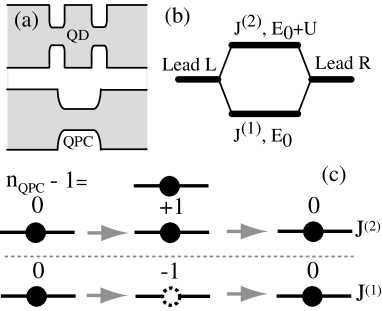
Figure 1: (a) Schematic view of a QD coupled to a QPC. (b) The two-channel model of the QPC. It consists of two conducting channels due to s-d coupling constants $J^{(i)}(i=1,2)$, which work as an Aharonov-Bohm interferometer in the QPC. (c) The charge fluctuations due to the transmission through the $J^{(1)}$ and $J^{(2)}$ channels. The numbers indicate $n_{\rm QPC}-1$.

The model Hamiltonian of the QPC proposed in Ref. Meir_2002 is the generalized s-d model: $H_{\rm QPC}=H_{\rm Lead}+H_{\rm sd}$ with

$$H_{\rm Lead}=\sum_{k\sigma\in L,R}\varepsilon_{k\sigma}\bar{c}_{k\sigma}c_{k\sigma},$$ (4)

$$H_{\rm sd} = \sum_{k,k^{\prime}\sigma\in L,R}(J^{(1)}_{kk^{\prime}}-J^{(2)}_{kk})\bar{c}_{k\sigma}c_{k^{\prime}\sigma}$$ (5)

$$+ 2\!\!\!\sum_{k,k^{\prime}\sigma\sigma^{\prime}\in L,R}(J^{(1)}_{kk^{\prime}}+J^{(2)}_{kk^{\prime}})\bar{c}_{k\sigma}\vec{\sigma}_{\sigma\sigma^{\prime}}c_{k^{\prime}\sigma^{\prime}}\cdot\vec{S},$$

where

$$J^{(i)}_{kk^{\prime}}=\frac{(-1)^{(i+1)}}{4}\left[\frac{V^{(i)}_{k}V^{(i)}_{k^{\prime}}}{\varepsilon_{k}-E^{(i)}}+\frac{V^{(i)}_{k}V^{(i)}_{k^{\prime}}}{\varepsilon_{k^{\prime}}-E^{(i)}}\right],$$ (6)

and $\bar{c}_{k\sigma}$ creates an electron with momentum $k$ and spin $\sigma$ in lead $L$ and $R$; $E^{(1)}=E_{0}$ and $E^{(2)}=E_{0}+U$ with the energy level of local spin state $E_{0}$ and the Coulomb energy $U$. $\vec{S}$ is the local spin due to the localized state. We assume $J_{kk^{\prime}}^{(i)}=J^{(i)}$. The exponential increase of the couplings is modeled by a Fermi function $f_{\rm FD}(x)=1/[1+\exp(x)]$, leading to the Fermi energy $E_{F}$ dependence of $J^{(i)}$: $J^{(i)}=\frac{(-1)^{(i+1)}(V^{(i)})^{2}}{E_{F}-E^{(i)}}f_{\rm FD}(-E_{F}/\delta).$

The Hamiltonian of the QD is the conventional Anderson model: $H_{QD}=\sum_{k,\sigma,\atop\alpha=L,R}\epsilon_{k}\bar{f}_{k\sigma\alpha}f_{k\sigma\alpha}+\sum_{\sigma}\varepsilon_{0}\bar{d}_{\sigma}d_{\sigma}+U_{d}n_{\uparrow}n_{\downarrow}+V_{T}\sum_{k,\sigma,\atop\alpha=L,R}\left[\bar{f}_{k\sigma\alpha}d_{\sigma}+{\rm h.c.}\right]$, where $\bar{d}_{\sigma}$ creates an electron in the QD with spin $\sigma$, while $\bar{f}_{k\sigma\alpha}$ creates an electron with momentum $k$ and spin $\sigma$ in the lead $\alpha$ attached to the QD with the tunneling matrix element $V_{T}$; $n_{\sigma}=\bar{d}_{\sigma}d_{\sigma}$, and $\varepsilon_{0}$ and $U_{d}$ are the energy level and the Coulomb energy in the QD, respectively.

The third part of the Hamiltonian, $H_{\rm QPC-QD}$ describes the interaction between the QPC and the QD. Localized electrons in the QPC interact with the electrons in the QD:

$$H_{\rm QPC-QD}=Wn_{\rm QPC}\sum_{\sigma}n_{\sigma},$$ (7)

where $n_{\rm QPC}$ is the number of localized electrons in the QPC, and $W$ is the coupling constant. The energy level in the QD is shifted by $H_{\rm QPC-QD}$: $\varepsilon_{0}\rightarrow\varepsilon_{0}+Wn_{\rm QPC}$.

Two channel induced dephasing. The conductance through the QPC was calculated using second order perturbation theory Meir_2002 ; Appelbaum : $G_{\rm QPC}=2e^{2}T/h$ with

$$T = 4\pi^{2}(\rho_{L}\rho_{R})^{2}\left((J^{(1)}-J^{(2)})^{2}+3(J^{(1)}+J_{r}^{(2)})^{2}\right)$$ (8)

and the density of states $\rho_{L}(\rho_{R})$ in the left (right) leads. We have introduced a renormalized coupling constant $J_{2;r}=1/[4\log(T/T_{K})]$ with the Kondo temperature $T_{K}=U\exp[-1/(4\rho J_{2})]$ that characterizes the Kondo effect in the QPC Meir_2002 . The right-hand side of Eq. (8) consists of three terms proportional to $(J^{(1)})^{2}$, $(J^{(2)})^{2}$, and $J^{(1)}J^{(2)}$. This combination of the terms indicates an AB interferometer picture with the $J^{(1)}$ and $J^{(2)}$ channels in the QPC as depicted in Fig. 1 (b). Note that the appearance of the $J^{(1)}J^{(2)}$ term is not peculiar to the s-d model (5). When multi channels involve electron transport, interference between them occurs.

The electron transport through the QPC induces fluctuations of $n_{\rm QPC}$ since it takes place via the co-tunneling processes described by $J^{(i)}$ in Eq. (6). If no current flows through the QPC, $n_{\rm QPC}=1$. When electrons pass through the $J^{(1)}$ channel, virtual excitations from $n_{\rm QPC}=1$ to $n_{\rm QPC}=0$ are involved, while when electrons pass through the $J^{(2)}$ channel, excitations to $n_{\rm QPC}=0$ are involved. These situations are depicted in Fig. 1 (c) with $n_{\rm QPC}-1$. This change in $n_{\rm QPC}$ shifts $\varepsilon_{0}$ in the QD. In this way, the transmission of electrons through the QPC is monitored by electrons in the QD. The current fluctuations (shot noise) through the QPC lead to fluctuations in $n_{\rm QPC}$ and eventually in $\varepsilon_{0}$. It has been shown that the fluctuations of $\varepsilon_{0}$ due to the external environment lead to dephasing in the QD, where the time evolution of $d_{\sigma}$ shows a exponential decay due to the fluctuations Levinson97 .

Transport through the “AB ring” in the QPC is monitored by the QD through these charge fluctuations. The terms proportional to $(J^{(1)})^{2}$ and $(J^{(2)})^{2}$ give the transmission probability with $n_{\rm QPC}-1=\mp 1$, respectively. These processes are monitored by the QD. The $J^{(1)}J^{(2)}$ term, on the other hand, describes the interference between the excited states with $n_{\rm QPC}-1=\pm 1$. This indicates that the term, compared to the $(J^{(1)})^{2}$ and $(J^{(2)})^{2}$ terms, involves smaller charge change in $n_{\rm QPC}$ after an electron passes through the QPC. In other words, the current fluctuations of the $(J^{(i)})^{2}$ terms contribute to the dephasing in the QD while those of the $J^{(1)}J^{(2)}$ term can be negligible.

The dephasing rate $\gamma$ is then the sum of the dephasing rates of the two independent channels, $(J^{(1)})^{2}$ and $(J^{(1)})^{2}$ terms. In each channel, we use the result of the previous theories Buks98 ; Aleiner97 ; Levinson97 ; Hackenbroich for a single channel QPC model. The measured $\Delta T$ characterizes the interaction between the QPC and QD. The total dephasing rate $\gamma$ is, instead of Eq. (1),

$$\gamma=\frac{eV_{\rm QPC}}{8\pi}\left[\gamma_{0}(T_{1})+\gamma_{0}(T_{2})\right]$$ (9)

with $\gamma_{0}(T)=[\Delta T(T)]^{2}/T(1-T),$ where $T_{i}$ is the transmission probability through the channel $J^{(i)}$:

$$T_{1/2} = 4\pi^{2}(\rho_{L}\rho_{R})^{2}(J_{1/2}^{2}+3J_{1/2r}^{2}).$$ (10)

The common factor of $\Delta T(T)$ appears for both transmission channels. This is because $\Delta T$ is measured by adding an electron to the QD, and this affects both channels equally.

We calculate $\gamma$ in Eq. (9) as a function of $T$ in Eq. (8). We use a perturbative approach with

$$\bar{T}=\frac{T}{1+T},$$ (11)

and

$$\bar{T}_{i}=\frac{T_{i}}{1+T_{i}},$$ (12)

in place of $T$ and $T_{i}$. This corresponds to taking into account the perturbative corrections to $H_{\rm Lead}$ by $H_{\rm sd}$. The current though the QPC is calculated in the following way. We expand the Keldysh action ${\rm T_{c}}\exp(-iS_{\rm sd}),$ where $S_{\rm sd}$ is the action of the s-d interaction (5), and the time order is taken along the Keldysh contour. We expand the action up to the second order in $J^{(i)}$, and reduce it to the bilinear form with respect to conduction electron fields using Wick’s theorem decoupling . Then we have a non-interacting model without $H_{\rm sd}$ and with the renormalized action $\tilde{S}_{0}$ for the kinetic term of conduction electrons. Then the current through the QPC is calculated with $\tilde{S}_{0}$ and the current operator $I=ie/\hbar[\sum_{k\in L,k^{\prime}\in R,\sigma}(J^{(1)}-J^{(2)})\bar{c}_{k\sigma}c_{k^{\prime}\sigma}+2\sum_{k,\sigma\in L,\atop k^{\prime}\sigma^{\prime}\in R}(J^{(1)}+J^{(2)})\bar{c}_{k\sigma}\vec{\sigma}_{\sigma\sigma^{\prime}}c_{k^{\prime}\sigma^{\prime}}\cdot\vec{S}]+{\rm h.c.}.$ The transmission probability is then given by Eq. (11). If the renormalization of $S_{0}$ is disregarded, where $\tilde{S}_{0}=S_{0}$ with the action $S_{0}$ for Eq. (4), the transmission probability is given by Eq. (8). The origin of $T$ in the denominator of Eq. (11) is the s-d scattering in each lead, while $T$ in the numerator is the scattering between two leads. Since the s-d coupling constants are equal for both scatting processes, the same factor of $T$ appears. In a similar way, the transmission probability $T_{i}$ through the channel $J^{(i)}$ acquires the denominator, $1+T_{i}$.

Comparison with experiment. We need to find the $T$ dependence of $\gamma_{0}$ from the experimental data. In Fig. 2(a), symbols indicate the two sets of the experimental data in Ref. Avinun04 . To fit these data, we use $\gamma_{0}(T)=0.9\sqrt{T/0.2}\times 10^{-5}$ when $T<0.2$ and $\gamma_{0}(T)=0.9\exp(1-(T/0.2)^{0.7})\times 10^{-5}$ when $T>0.2$. The plot is shown by the solid line in Fig. 2(a). This choice of $\gamma_{0}$ reflects the fact that $\Delta T$ is a highly asymmetric function with respect to $T$; The maximum of $\Delta T$ is located at $T=0.2$. Other choices of $\gamma_{0}$ will give qualitatively similar results.

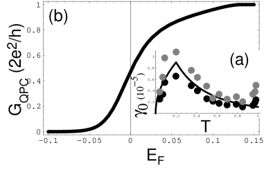
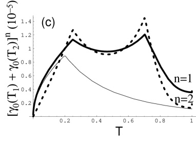
Figure 2: (a) $\gamma_{0}$ as a function of $T$. Symbols indicate the experimental data in Ref. Avinun04 . The solid line is the fitting curve. (b) $G_{\rm QPC}$ as a function of the Fermi energy $E_{F}$ of conduction electrons with $\rho(V^{(1)})^{2}=0.25,\rho(V^{(2)})^{2}=0.025,U=1.5,\delta=0.02,k_{B}T=0.001$. The unit of energy is $|E_{0}|$. (c) $[\gamma_{0}(T_{1})+\gamma_{0}(T_{2})]^{n}$ as a function of $T$. The thick solid line ($n=1$) is for Eq. 9 while the thin line is for the conventional QPC model, and the broken line ($n=2$) for Kang’s result Kang .

In the experiments, the differential conductance through the QPC exhibited a zero bias anomaly (ZBA) while no clear sign of the 0.7 structure was observed. In Ref. Cronenwett , a ZBA was observed, which confirms that it originates from the Kondo effect. The absence of a clear 0.7 structure does not contradict the Kondo effect but rather it indicates that the effect is strong. In Fig. 2(b), $G_{\rm QPC}$ is plotted as a function of the Fermi energy $E_{\rm F}$ of conduction electrons with $\rho(V^{(1)})^{2}/|E_{0}|=0.25,\rho(V^{(2)})^{2}/|E_{0}|=0.025$, and $U/|E_{0}|=1.5$. The parameters are chosen so that the QPC does not show a clear 0.7 structure in $G_{\rm QPC}$.

In Fig. 2(c), $\gamma/(eV_{\rm QPC}/8\pi)=\gamma_{0}(T_{1})+\gamma_{0}(T_{2})$ is plotted as a function of $T$ by the thick solid line, while for comparison $\gamma_{0}(T)$ for the conventional single channel QPC model is shown by the thin solid line. A double peak structure of $\gamma$ appears as in the experiment, in contrast to a single peak structure. The peak positions are located at $T\sim 0.25$ and $T\sim 0.7$. According to Ref. Kang , $\Delta G$ is given by Eq. (3). It is proportional to $\gamma^{2}\propto[\gamma_{0}(T_{1})+\gamma_{0}(T_{2})]^{2}$ when $\gamma\ll T_{K}$. The broken line in Fig. 2 (c) shows the result for this case. The double peak structure becomes more pronounced.

We should mention a consequence of the asymmetric line shape of $\Delta T$, which questions the dephasing theory based on the conventional model of the QPC. The dephasing rate is too small when $T\sim 0.7$ besides the absence of the extra peak. If $\Delta T$ were symmetric, $\gamma_{0}(T)$ would be symmetric around $T=1/2$. The difference between the experiment and theory was then quantitative, but not qualitative. The experiment revealed an essential feature of the QPC. For the two channel model used here, on the other hand, this asymmetry helps to show the double peak structure.

Discussion. If the 0.7 structure of $G_{\rm QPC}$ is observed, the second peak near $T=0.7$ of $\gamma$ is sharper than the one without the 0.7 structure. This is because the conductance is changed noticeably near $T=0.7$, and then the shot noise through the $J^{(2)}$ channel changes abruptly as well.

We did not address the amplitude of $\Delta G$. As pointed out by Kang Kang , the asymmetrical structure of the QPC induces an larger dephasing rate in the experiment. In this case, the dephasing rate depends on not only $\Delta T$ but also on the change of the phase shift through the QPC, which requires additional information from experiments, such as measurements in the device setup in Ref. Sprinzak .

In conclusion, we have discussed the dephasing mechanism due to charge fluctuations of a quasi-bound state in a quantum point contact. The bound state is responsible for there being two transmission channels. The dephasing rate is proportional to the sum of the transmission probability through these two channels. This mechanism explains the double peak structure of the suppression rate of the conductance, observed in a recent experiment Avinun04 . The result is qualitatively different from the rate without the bound state in the QPC.

The author acknowledges fruitful discussions with Y. Meir, as well as valuable comments on the manuscript. He also thanks to M. Avinun-Kalish, Y. Dubi, A. Golub, T. Rejec, and R. S. Tasgal for discussions.

References

- (1) A. Yacoby et al., Phys. Rev. Lett. 74 (1995) 4047.
- (2) R. Schuster et al., Nature 385 (1997) 417.
- (3) E. Buks et al., Nature 391, 871 (1998).
- (4) D. Sprinzak et al., Phys. Rev. Lett. 84, 5820 (2000).
- (5) I. L. Aleiner, N. S. Wingreen, and Y. Meir, Phys. Rev. Lett. 79 (1997) 3740.
- (6) Y. Levinson, Europhys. Lett. 39 (1997) 299.
- (7) G. Hackenbroich, B. Rosenow, and H. A. Weidenmüller, Phys. Rev. Lett. 81 (1998) 5896; G. Hackenbroich, Phys. Rep. 343, 463 (2001).
- (8) M. Avinun-Kalish et al., Phys. Rev. Lett. 92, 156801 (2004).
- (9) A. Silva and S. Levit, Europhys. Lett. 62, 103 (2003).
- (10) K. Kang, Phys. Rev. Lett. 95, 206808 (2005).
- (11) K. J. Thomas et al., Phys. Rev. Lett. 77, 135 (1996).
- (12) K. J. Thomas et al., Phys. Rev. B 58, 4846 (1998).
- (13) A. Kristensen et al., Phys. Rev. B 62, 10950 (2000).
- (14) D. J. Reilly et al., Phys. Rev. B 63, 121311(R) (2001).
- (15) S. M. Cronenwett et al., Phys. Rev. Lett. 88, 226805 (2002).
- (16) D. J. Reilly et al., Phys. Rev. Lett. 89, 246801 (2002).
- (17) A. C. Graham et al., Phys. Rev. Lett. 91, 136404 (2003).
- (18) L. P. Rokhinson, L. N. Pfeiffer, and K. W. West, Phys. Rev. Lett. 96, 156602 (2006).
- (19) T. Morimoto, et al., Phys. Rev. Lett. 97, 096801 (2006).
- (20) R. Crook et al., Science 312, 1359 (2006).
- (21) S. Lüscher et al., Phys. Rev. Lett. 98, 196805 (2007).
- (22) K. A. Matveev, Phys. Rev. Lett. 92, 106801 (2004); Phys. Rev. B 70, 245319 (2004).
- (23) D. J. Reilly, Phys. Rev. B 72, 033309 (2005).
- (24) H. Bruus, V. V. Cheianov, and K. Flensberg, Physica E 10, 97 (2001).
- (25) Y. Tokura and A. Khaetskii, Physica E 12, 711 (2004).
- (26) P. S. Cornaglia and C. A. Balseiro, Europhys. Lett. 67, 634 (2004).
- (27) M. Kindermann, P. W. Brouwer, and A. J. Millis, Phys. Rev. Lett 97, 036809 (2006); M. Kindermann, and P. W. Brouwer, Phys. Rev. B 74, 125309 (2006).
- (28) K.-F. Berggren and I. I. Yakimenko, Phys. Rev. B 66, 085323 (2002).
- (29) K. Hirose, Y. Meir, and N. S. Wingreen, Phys. Rev. Lett. 90, 026804 (2003).
- (30) P. Jaksch, I. I. Yakimenko, and K.-F. Berggren, Phys. Rev. B 74, 235320 (2006).
- (31) T. Rejec and Y. Meir, Nature 442, 900 (2006).
- (32) S. Ihnatsenka, I. V. Zozoulenko, cond-mat/0703380v1.
- (33) Y. Meir, K. Hirose, and N. S. Wingreen, Phys. Rev. Lett. 89, 196802 (2002).
- (34) P. Roche et al., Phys. Rev. Lett. 93, 116602 (2004).
- (35) L. DiCarlo et al., Phys. Rev. Lett. 97, 036810 (2006).
- (36) A. Golub, T. Aono, and Y. Meir Phys. Rev. Lett. 97, 186801 (2006).
- (37) J. A. Appelbaum, Phys. Rev. Lett. 17, 91 (1966); Phys. Rev. 154, 633 (1967).
- (38) It is useful to apply a unitary transformation for the conduction electrons, introducing two linear combinations of and , where and . Then the latter is decoupled from the s-d interaction. See also, Ref. Golub06 .