Microlensing Detections of Planets in Binary Stellar Systems

Abstract

We demonstrate that microlensing can be used for detecting planets in binary stellar systems. This is possible because in the geometry of planetary binary systems where the planet orbits one of the binary component and the other binary star is located at a large distance, both planet and secondary companion produce perturbations at a common region around the planet-hosting binary star and thus the signatures of both planet and binary companion can be detected in the light curves of high-magnification lensing events. We find that identifying planets in binary systems is optimized when the secondary is located in a certain range which depends on the type of the planet. The proposed method can detect planets with masses down to one tenth of the Jupiter mass in binaries with separations $\lesssim 100$ AU. These ranges of planet mass and binary separation are not covered by other methods and thus microlensing would be able to make the planetary binary sample richer.

1. Introduction

A binary star system is the most common result of star formation process. As the majority of stars belong to double or multiple star systems (Duquennoy & Mayor, 1991; Eggenberger et al., 2004), it is important to study the frequency of planets in binary systems and the properties of these planets for better understanding of the process of planet formation and evolution.

Planets in binaries have been discovered mainly through two channels. The first one is to perform dedicated surveys looking for planets in known visual or spectroscopic binaries (Konacki, 2005; Desidera et al., 2006; Eggenberger et al., 2006). The second approach is to study the binarity of the hosts of planets discovered in planet surveys (Patience et al., 2002; Eggenberger et al., 2004). We now know $\sim 40$ planets in binaries or multiple systems. These systems are mostly wide binaries with separations of several hundred to several thousand AU.

However, the sample of planets in binaries is not still large enough for the statistical analysis of their properties. This is because binaries with separations $\lesssim 100$ AU are difficult targets for radial velocity surveys, which is the most productive technique among those currently being used for planet searches, and thus were often rejected from the samples. In addition, due to the limitations of the available observational techniques, most detected objects are giant (Jupiter-like) planets, implying that the existence of smaller mass planets in multiple star systems is still an open question.

In this paper, we demonstrate that microlensing technique can be used for detecting planets in binary systems, especially for low-mass planets in binaries with separations $\lesssim 70$ AU. In the geometry of planets in binary systems where the planet orbits one component of a binary and the other binary star is located at a large distance, perturbations induced by the planet and binary companion can occur in the same region around the planet-hosting binary component. Then, the signatures of both planet and binary companion can be identified in the light curve of a lensing event produced by the source star’s passage close to the star hosting the planet.

The paper is organized as follows. In § 2, we describe lensing properties in various cases of lens geometry, including binary, planetary, and triple lensing. In § 3, we describe the channels of lensing events from which planets in binaries can be detected. We illustrate signatures of planets in binary stellar systems and investigate the range of binary separations within which detections of planets are optimized. We also discuss about possible complications in the interpretation of the signals. We summarize and conclude in § 4.

Figure 1.— Magnification patterns of triple lens systems composed of a planet and binary stars. The coordinates are centered at the position of the planet-hosting star (primary) and the $x$-axis is aligned with the line connecting the primary and the other binary star (secondary). All lengths are in units of the Einstein radius corresponding to the mass of the primary star, $\theta_{\rm E,1}$. The secondary is on the right side and the position angle of the planet measured from the primary-secondary axis is $60^{\circ}$. The projected distances of the planet ($\hat{s}_{\rm p}$) and secondary ($\hat{s}_{\rm b}$) from the primary are marked in each panel. Note that notations with the hat represent length scales normalized by $\theta_{\rm E,1}$. Also marked are the mass ratios of the planet-primary ($q_{\rm p}$) and secondary-primary ($q_{\rm b}$) pairs. Panels in each column show the magnification patterns of lens systems with a common planet but with different separations to the secondary star. Panels in each row show the cases where the size of the planet-induced caustic $\Delta\xi_{\rm c,p}$ is two times smaller (upper row), equivalent (middle row), and two times larger (lower row) than the size of the secondary-induced caustic $\Delta\xi_{\rm c,b}$, respectively. Brighter greyscale represents the region of higher magnifications. The figures drawn in soild curves are the caustics. The straight lines with arrows represent source trajectories and the light curves of the resulting events are presented in the corresponding panels of Figure 3 (solid curves).

2. Multiple Lensing

The lensing behavior of a planet in a binary stellar system requires the formalism of a triple lens with two equivalent-mass components and a very low-mass third body. If a source star is gravitationally lensed by a lens system composed of $N$ point-masses, the equation of lens mapping from the lens plane to the source plane (lens equation) is expressed as (Witt, 1990)

$$\zeta=z-\sum_{j=1}^{N}{m_{j}/M\over\bar{z}-\bar{z}_{{\rm L},j}},$$ (1)

where $\zeta=\xi+i\eta$, $z_{{\rm L},j}=x_{{\rm L},j}+iy_{{\rm L},j}$, and $z=x+iy$ are the complex notations of the source, lens, and image positions, respectively, $\bar{z}$ denotes the complex conjugate of $z$, $m_{j}$ are the masses of the individual lens components, and $M=\sum_{j}m_{j}$ is the total mass of the system. Here all lengths are normalized to the Einstein radius corresponding to the total mass of the lens system, i.e.

$$\theta_{\rm E}=\left[{4GM\over c^{2}}\left({1\over D_{\rm L}}-{1\over D_{\rm S}}\right)\right]^{1/2},$$ (2)

where $D_{\rm L}$ and $D_{\rm S}$ are the distances to the lens and source, respectively. Finding the locations of images for a given positions of the lens and source requires inversion of the lens equation. The lensing process conserves the source surface brightness and thus the magnifications $A_{i}$ of the individual images correspond to the ratios between the areas of the images and source. For each image located at $z_{i}$, this ratio corresponds to the Jacobian of the lens equation, i.e.

$$A_{i}=\left|\left(1-{\partial\zeta\over\partial\bar{z}}{\overline{\partial\zeta}\over\partial\bar{z}}\right)_{z=z_{i}}^{-1}\right|.$$ (3)

For Galactic microlensing events, the typical separation between images is of the order of 0.1 mill-arcsec and thus the individual images cannot be resolved. However, events can be noticed by the variation of the source star flux (Paczyński, 1986), where the magnification corresponds to the sum of the magnifications of the individual images, i.e. $A=\sum_{i}A_{i}$.

For a single-lens case, the lens equation is simply inverted to solve the image positions. This yields two images located at

$${\bf u}_{{\rm I},\pm}={1\over 2}\left[u\pm(u^{2}+4)^{1/2}\right]{{\bf u}\over u},$$ (4)

where ${\bf u}=\mbox{\boldmath$\zeta$}-{\bf z}_{\rm L}$ is the separation vector between the lens and source. The magnifications of the individual images are

$$A_{\pm}={1\over 2}\left[{u^{2}+2\over u(u^{2}+4)^{1/2}}\pm 1\right],$$ (5)

yielding a total magnification of

$$A=A_{+}+A_{-}={u^{2}+2\over u(u^{2}+4)^{1/2}}.$$ (6)

If a lens system is composed of more than two masses, the lens equation cannot be inverted algebraically. One way to investigate the lensing optics for a multiple-lens system is expressing the lens equation as a polynomial in $z$ and finding the image positions by numerically solving the polynomial (Witt & Mao, 1995). The advantage of this method is that it allows semi-analytic description of the lensing behavior and saves computation time. However, the order of the polynomial increases as $N^{2}+1$ and thus solving the polynomial becomes difficult as the number of lenses increases. In this case, one can still obtain the magnification patterns by using the inverse ray-shooting technique (Schneider & Weiss, 1986; Kayser, Refsdal & Stabell, 1986; Wambsganss, Paczyński & Schneider, 1990). In this method, a large number of light rays are uniformly shot backwards from the observer plane through the lens plane and then collected (binned) in the source plane. Then, the magnification pattern is obtained by the ratio of the surface brightness (i.e., the number of rays per unit area) on the source plane to that on the observer plane. Once the magnification pattern is constructed, the light curve resulting from a particular source trajectory corresponds to the one-dimensional cut through the constructed magnification pattern. Although this methods requires a large amount of computation time for the construction of the detailed magnification pattern, it has the advantage that the lensing behavior can be investigated regardless of the number of lenses.

Figure 2.— Magnification patterns of lens systems composed of binary stars but without planets. The notations are same as those in Figure 1. The light curves resulting from the source trajectories marked in the individual panels are presented in the corresponding panels of Figure 3 (dotted curves).

The number of images, their locations, and the resulting magnification pattern vary greatly depending on the number of lenses, their individual mass fractions, and the geometry of the lens system. A multiple-lens system has a maximum of $N^{2}+1$ images and a minimum of $N+1$ images. One common important characteristic of multiple lensing is the formation of caustics. Caustics represent the set of source positions at which the magnification of a point source becomes infinite. For a binary-lens case, the caustic form a single or multiple sets of closed curves each of which is composed of concave curves (fold caustics) that meet at points (cusps). Unlike the caustics of binary lensing, caustics of multiple lensing can exhibit self-intersecting and nesting. The number of images changes by a multiple of two as the source crosses a caustic (Rhie, 1997).

3. Signatures of Planet and Binary Companion

3.1. Perturbation Approach

We consider the geometry of planets in binary stellar systems where the planet is orbiting one of the star in the binary and the other binary star is located at a larger distance. Hereafter we refer the star hosting the planet as primary and the other binary star as secondary. In this lens geometry, the resulting lensing behavior can be approximated as the superposition of those of the binary lens pairs composed of the primary-secondary stars and primary-planet. This is possible because the lensing effects caused by the secondary star and the planet in the region around the primary star are small and thus can be treated as perturbations. For the primary-secondary pair, the effect of the secondary is small because of the large distance to the secondary star (Dominik, 1999). For the primary-planet pair, on the other hand, the effect of the planet is small because of the small mass ratio of the planet (Bozza, 1999).

Figure 3.— Light curves of events resulting from the source star trajectories marked on the magnification pattern maps in Figure 1 and 2. Solid and dotted curves are the light curves with and without the planet, respectively. For the construction of the light curves, finite-source effect is taken into consideration by assuming that the source star radius normalized by the Einstein radius is $\rho_{\star}=0.002$. Time scale is normalized by the Einstein time scale corresponding to the mass of the primary.

In the limiting case of a binary lens where the projected separation between the lens components is much larger than the Einstein radius, the lensing behavior in the vicinity of the primary star is approximated by the equation of the Chang-Refsdal lensing (Chang & Refsdal, 1979, 1984; Dominik, 1999), i.e.

$$\hat{\zeta}=\hat{z}-{1\over\hat{z}}+\gamma\hat{z}.$$ (7)

Here the notations with the ‘hat’ represent length scales normalized by the Einstein radius corresponding to the mass of the primary star, $\theta_{{\rm E},1}=\theta_{\rm E}[m_{1}/(m_{1}+m_{2})]^{1/2}$, $m_{1}$ and $m_{2}$ are the masses of the primary and companion stars, respectively, and $\gamma$ represents the shear induced by the secondary star. The shear is related to the binary parameters by

$$\gamma={q_{\rm b}\over\hat{s}_{\rm b}^{2}};\qquad q_{\rm b}={m_{2}\over m_{1}},$$ (8)

where $\hat{s}_{\rm b}$ is the separation between the binary stars normalized by $\theta_{\rm E,1}$. The validity of equation (7) implies that if the binary separation is sufficiently wide ($s_{\rm b}\gg 1.0$), the lensing behavior in the region around the primary star can be approximated as that of a single point-mass lens superposed on a uniform background shear $\gamma$. The result of the external shear is manifested as the formation of a small caustic around the primary with the shape of a hypocycloid with four cusps. The width of the caustic as measured by the separation between the two cusps located on the binary axis is

$$\Delta\xi_{\rm c,b}\simeq{4\gamma\over(1-\gamma)^{1/2}}={4q_{\rm b}\over\hat{s}_{\rm b}^{2}}\left(1+{q_{\rm b}\over 2\hat{s}_{\rm b}^{2}}\right).$$ (9)

The caustic is tiny for a wide-separation binary because its size shrinks as $\Delta\xi_{\rm c,b}\propto\hat{s}_{\rm b}^{-2}$. However, a perturbation can occur if the source trajectory approaches close enough to the primary lens around which the caustic is located. During the time of perturbation, the source star is close to the primary lens and thus the magnification of the resulting event is very high. Then, the signature of a wide-separation secondary is a short-duration perturbation near the peak of the light curve of a high-magnification event (Han & Kang, 2003).

Because of the small mass ratio of the planet, the light curve of a planetary lensing event is also well described by that of a single lens of the primary star for most of the event duration. For a planetary case, there exist two sets of disconnected caustics. Among them, one is located away from the primary star. The other caustic, on the other hand, is located close to the primary lens. The caustic located close to the primary (central caustic) has a wedge-like shape and its size as measured by the width along the star-planet axis (Chung et al., 2005) is related to the planet parameters by

$$\Delta\xi_{\rm c,p}\simeq{4q_{\rm p}\over(s_{\rm p}-1/s_{\rm p})^{2}};\qquad q_{\rm p}={m_{\rm p}\over m_{1}},$$ (10)

where $s_{\rm p}$ is the separation between the primary and planet measured in units of $\theta_{\rm E}$ and $m_{\rm p}$ is the mass of the planet. We note that for the case of a planetary lensing where $q_{\rm p}\ll 1.0$, $\theta_{\rm E}\sim\theta_{\rm E,1}$ and thus $s_{\rm p}\sim\hat{s}_{\rm p}$. The size of the caustics is maximized when the planet is located close to the Einstein ring of the primary star, $s_{\rm p}\sim 1.0$. Since the central caustic is located close to the primary lens, the perturbation region around the central caustic induced by the planet overlaps with the perturbation region induced by the wide-separation binary companion.

3.2. Optimal Lens Geometry

Because the planet-induced perturbation region overlaps with the perturbation region caused by a wide-separation secondary, the deviation induced by the planet can be additionally perturbed by the binary companion. This makes it possible to use the microlensing technique as a tool to identify planets in binary systems.

To illustrate the feasibility of the microlensing detection of planets in binary stars, we present magnification patterns of triple lens systems composed of a planet and binary stars in Figure 1. In each map, the coordinates are centered at the position of the primary and the $x$-axis is aligned with the primary-secondary axis. Since the perturbation occurs near the peak of a seemingly single-lens event caused by the primary, we normalize all lengths in units of the Einstein radius corresponding to the mass of the primary star. The secondary is on the right side and the position angle of the planet measured from the primary-secondary axis is $60^{\circ}$. The separations to the planet ($\hat{s}_{\rm p}$) and secondary ($\hat{s}_{\rm b}$) are marked in each panel. Also marked are the mass ratios of the planet-primary ($q_{\rm p}$) and secondary-primary ($q_{\rm b}$) pairs. Panels in each column show the magnification patterns of lens systems with a common planet but with different projected distances to the secondary star. Panels in each row show the cases where the size of the planet-induced caustic $\Delta\xi_{\rm c,p}$ is two times smaller (upper row), equivalent (middle row), and two times larger (lower row) than the size of the secondary-induced caustic $\Delta\xi_{\rm c,b}$, respectively. Brighter greyscale represents the region of higher magnifications. The figures drawn in solid curves represent the caustics. Note that the caustic curves exhibit self-intersecting and nesting, that are the characteristics of multiple lensing. In Figure 2, we also present maps of binary lenses without planet for the comparison of the patterns with the triple-lens systems. The straight lines with arrows in the magnification pattern maps represent source trajectories and the light curves of the resulting events are presented in the corresponding panels of Figure 3. Since both caustics induced by the planet and secondary companion are small, finite size of the source star would be important in lensing light curves. We therefore consider the finite-source effect by assuming that the source star has a radius equivalent to the Sun, i.e. $r_{\star}=1\ R_{\odot}$. For a typical Galactic event caused by a low-mass stellar object of $m_{1}=0.3\ M_{\odot}$ and with distances to the lens and source stars of $D_{\rm L}=6$ kpc and $D_{\rm L}=8$ kpc, respectively, the angular Einstein radius is $\theta_{\rm E}=0.32$ mas and the radius of the source star normalized to the Einstein radius is $\rho_{\star}\sim 0.002$. For other combinations of the lens and source parameters, the normalized source size is

$$\rho_{\star}=0.0009\left({r_{\star}\over R_{\odot}}\right)\left({0.3\ M_{\odot}\over M}\right)^{1/2}\left({D_{\rm L}\over 6\ {\rm kpc}}\right)^{1/2}\left(1-{D_{\rm L}\over D_{\rm S}}\right)^{-1/2}.$$ (11)

For the construction of the magnification maps and light curves, we use the inverse ray-shooting technique due to the difficulty in solving tenth-order triple-lens polynomial lens equation incorporating finite-source effect.

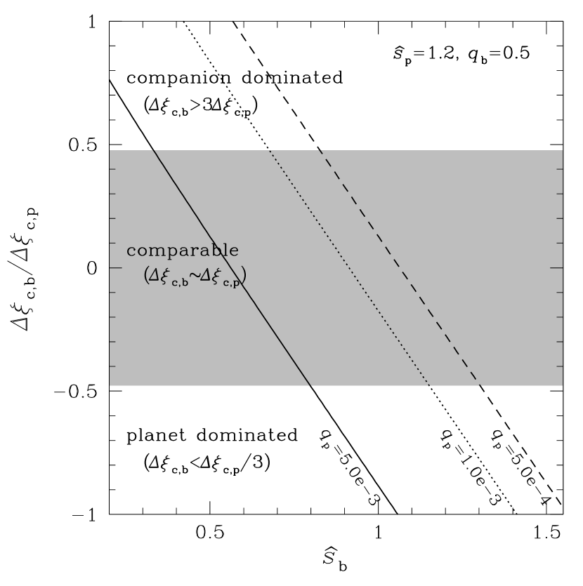
Figure 4.— Size ratio between the caustics induced by the planet ($\Delta\xi_{\rm c,p}$) and secondary companion ($\Delta\xi_{\rm c,b}$) in triple lens systems composed of a planet and binary stars as a function of the separation between the primary and secondary star. The shaded area represents the region where the ratio is $1/3\leq\Delta\xi_{\rm c,b}/\Delta\xi_{\rm c,p}\leq 3$. The binary separation $\hat{s}_{\rm b}$ is normalized by the Einstein radius corresponding to the mass of the primary star. To draw the curve, we adopt a distance to the planet of $\hat{s}_{\rm p}=1.2$ and a secondary/primary mass ratio of $q_{\rm b}=0.5$ as representative values. Note that notations with hat represent length scales normalized to the Einstein radius corresponding to the mass of the planet-hosting star.

Table 1Optimal Binary Separation

planet	optimal range of secondary separation
mass ratio	normalized unit	physical unit
$5.0\times 10^{-3}$	$2.1\lesssim\hat{s}_{\rm b}\lesssim 6.7$	$4.2\ {\rm AU}\lesssim d_{\rm b}\lesssim 13.4\ {\rm AU}$
$1.0\times 10^{-3}$	$4.8\lesssim\hat{s}_{\rm b}\lesssim 14.2$	$9.2\ {\rm AU}\lesssim d_{\rm b}\lesssim 28.4\ {\rm AU}$
$5.0\times 10^{-4}$	$6.7\lesssim\hat{s}_{\rm b}\lesssim 20.1$	$13.4\ {\rm AU}\lesssim d_{\rm b}\lesssim 65.2\ {\rm AU}$

Note. — Ranges of binary separation for optimal microlensing detections of planets in binaries. Here $\hat{s}_{\rm b}$ represents the binary separation normalized by the Einstein radius corresponding to the mass of the planet-hosting star. The physical separation $d_{\rm b}$ is determined by assuming that the physical Einstein radius is $r_{\rm E}=2.0$ AU.

From the figures, one finds that the magnification pattern of the binary star with a planet is different from either the primary-secondary or primary-planet pair and thus the resulting light curve can produce distinctive signatures in the lensing light curves. One also finds that identifying planets in binary systems is optimized when the secondary is located in a certain range of separation from the primary. This optimal separation range varies depending on the type of the planet. To produce noticeable planetary signature, planets should be located close to the Einstein ring of the primary star. Under this lens geometry, if the secondary is located not far enough from the primary, the perturbation induced by the secondary dominates over the planet-induced perturbation. If the secondary is located too far away from the primary, on the contrary, its signature would be too small to be noticed. Then, identifying the signatures of both planet and secondary would be optimized when the companion is located at a separation where the amount of secondary-induced perturbation is equivalent to that of the planet-induced perturbation. When the planet is located within this optimal range, we find that planets can be detected with mass ratios down to $q\sim 5\times 10^{-4}$, which corresponds to one tenth of the mass of the Jupiter.

In Figure 4, we present the size ratio between the caustics induced by the planet and secondary companion as a function of the binary separation. The curves with different line types show the ratios for planets with different mass ratios. To draw the curve, we adopt a planetary separation of $\hat{s}_{\rm p}=1.2$ and a binary mass ratio of $q_{\rm b}=0.5$ as representative values. The shaded area represents the region where the sizes of the two caustics induced by the planet and secondary are comparable and thus the chance of detecting the signatures of both planet and secondary is relatively high. In Table 1, we also present the optimal range of binary separations both in normalized and physical units. The physical separation is determined by assuming that the physical Einstein radius is $r_{\rm E}=D_{\rm L}\theta_{\rm E}=2.0$ AU. We find that although varies depending on the planet type, the optimal range of the binary separation for planet detection is $\lesssim 70$ AU. Binaries with separations in this range is not being covered by the current radial velocity method.

3.3. Interpretation of Signatures

Since the perturbations caused by the planet and the wide-separation binary companion occur in a common region and at a similar location of the lensing light curve, one might question whether the light curve produced by a binary lens with a planet could be mimicked by that of a simple binary-lens or a single planetary event by appropriate modification of the lens parameters. However, we note that although the perturbation regions induced by the planet and the companion are similar, they are not identical. As a result, the characteristic shape of the perturbation such as the multiple-peak features shown in Figure 3 cannot be produced by a single companion.

Another related question would be whether the light curve could be mimicked by that of an event caused by a single stellar lens with multiple planets (Gaudi et al., 1998). In this case, the light curve can exhibit multiple-peak features. However, the perturbations induced by planets in general have different characteristics from those induced by wide-separation companions and the two different types of perturbation can be well distinguished as demonstrated in practice for the case of the lensing event MACHO 99-BLG-47 (Albrow et al., 2002). In addition, the individual perturbations are in many cases well separated, allowing investigation of the individual perturbations (Han, 2005). Therefore, it would be possible to distinguish the two possible degenerate cases.

4. Conclusion

We demonstrated that microlensing technique can be used for the detections of planets in binary stellar systems, especially for low-mass planets in binaries with small separations. The signatures of both planet and binary companion can be detected in the light curve of a high-magnification lensing event. High-magnification events are the prime target of high-cadence follow-up microlensing observations currently being conducted to search for extrasolar planets (Abe et al., 2004; Cassan et al., 2004; Park et al., 2004) and two planets were actually detected through this channel (Udalski et al., 2005; Gould et al., 2006). We found that identifying planets in binary systems is optimized when the secondary is located in a certain range which depends on the type of the planet. The proposed method can detect planets with masses down to one tenth of the Jupiter mass in binaries with binary separations $\lesssim 100$ AU. These ranges of planet mass and binary separation are not covered by other methods and thus microlensing would be able to make the planetary binary sample richer.

References

- Abe et al. (2004) Abe, F., et al. 2004, Science, 305, 1264
- Albrow et al. (2002) Albrow, M. D., et al. 2002, ApJ, 572, 1031
- Bozza (1999) Bozza, V. 1999, A&A, 348, 311
- Cassan et al. (2004) Cassan, A., et al. 2004, A&A, 419, L1
- Chang & Refsdal (1979) Chang, K., & Refsdal, S. 1979, Nature, 282, 561
- Chang & Refsdal (1984) Chang, K., & Refsdal, S. 1984, A&A, 132, 168
- Chung et al. (2005) Chung, S.-J., et al. 2005, ApJ, 630, 535
- Desidera et al. (2006) Desidera, S., et al. 2006, Proc. of the conference Tenth Anniversary of 51 Peg-b: Status of and Prospects for Hot Jupiter Studies, 119
- Dominik (1999) Dominik, M. 1999, A&A, 349, 108
- Duquennoy & Mayor (1991) Duquennoy, A., & Mayor, M. 1991, A&A, 248, 485
- Eggenberger et al. (2004) Eggenberger, A., Halbwachs, J., Udry, S., & Mayor, M. 2004, Proc. of IAU Colloquium 191, 21, 28
- Eggenberger et al. (2004) Eggenberger, A., Udry, S., & Mayor, M. 2004, A&A, 417, 353
- Eggenberger et al. (2006) Eggenberger, A., Mayor, M., Naef, D., Pepe, F., Queloz, D., Santos, N. C., Udry, S., & Lovis, C. 2006, A&A, 447, 1159
- Gaudi et al. (1998) Gaudi, B. S., Naber, R. M., & Sackett, P. D. 1998, ApJ, 502, L33
- Gould et al. (2006) Gould, A., et al. 2006, ApJ, 644, L37
- Haghighipour (2006) Haghighipour, N. 2006, ApJ, 644, 543
- Han (2005) Han, C. 2005, ApJ, 629, 1102
- Han & Kang (2003) Han, C., & Kang, Y. W. 2003, ApJ, 596, 1320
- Kayser, Refsdal & Stabell (1986) Kayser R., Refsdal S., & Stabell R. 1986, A&A, 166, 36
- Konacki (2005) Konacki, M. 2005, Nature, 436, 230
- Paczyński (1986) Paczyński, B. 1986, 304, 1
- Park et al. (2004) Park, B.-G., et al. 2004, ApJ, 609, 166
- Patience et al. (2002) Patience, J., et al. 2002, ApJ, 581, 654
- Rhie (1997) Rhie, S. H. 1997, ApJ, 484, 63
- Schneider & Weiss (1986) Schneider P., & Weiss A. 1986, A&A, 164, 237
- Sigurdsson (1993) Sigurdsson, S. 1993, ApJ, 415, L43
- Wambsganss, Paczyński & Schneider (1990) Wambsganss J., Paczyński B., & Schneider P. 1990, ApJ, 358, L33
- Udalski et al. (2005) Udalski, A., et al. 2005, ApJ, 628, L109
- Witt (1990) Witt, H. J. 1990, A&A, 236, 311
- Witt & Mao (1995) Witt, H. J., & Mao, S. 1995, ApJ, 447, L105