Self-consistent theory of phonon renormalization and electron-phonon coupling near a 2D Kohn singularity

Abstract

We show that the usual expression for evaluating electron-phonon coupling and the phonon linewidth in 2D metals with a cylindrical Fermi surface cannot be applied near the wave vector corresponding to the Kohn singularity. Instead, the Dyson equation for phonons has to be solved self-consistently. If a self-consistent procedure is properly followed, there is no divergency in either the coupling constant or the phonon linewidth near the offending wave vectors, in contrast to the standard expression.

First principles calculations of the phonon spectra and electron-phonon coupling in MgB₂ (see Ref. MA for a review) have determined that the interaction mainly responsible for superconductivity in this material is coupling of small-$q$, high-energy optical phonons of a particular symmetry with approximately parabolic nearly two-dimensional hole bands forming practically perfect circular cylinders occupying only a small fraction of the Brillouin zone. It was realized early enoughkong that the case of an ideal 2D cylinder leads to a divergency in the calculated phonon linewidth at the 2D Kohn singularity, $q=2k_{F},$ which presents serious difficulties in calculating the electron-phonon coupling function. One option that was exploited was to use an analytical integration for the wave vectors comparable with, or smaller than $2k_{F}$kong ; amy , and a numerical one for the larger vectors.

It was also pointed outMA ; an that this singularity gets stronger when the Fermi surface gets smaller, while the integrated electron-phonon coupling (for 2D parabolic bands) does not change. While a perfectly cylindrical Fermi surface is an idealized construction, deviations may be quite small, it seems, on the first glance, unphysical that all phonons with $|\mathbf{q}|=2k_{F}$ have infinite linewidth. Note that the problem is not specific for MgB${}_{2}:$ it occurs for any 2D material sporting Kohn singularities. In particular, the hypothetical hexagonal LiB, a subject of a substantial recent interest, has $\sigma$ bands that are even more 2D that those in MgB₂ lib and the described problem is even more pronounced.

This intuition is correct. In this paper we show that close to a Kohn anomaly standard formulas for calculating electron-phonon interaction (EPI) become incorrect, and new, self-consistent expressions replace them. These expressions have no singularities, and exhibit a much more natural, reasonably smooth, q-dependence of the phonon self-energy.

To start with, we shall remind the readers the standard formalism. We first define the retarded phonon Green function

$$D^{\alpha\beta}\left(\mathbf{q},t\right)\equiv-i\theta(t)\left\langle\left[u_{\mathbf{q}}^{\alpha}(t)u_{-\mathbf{q}}^{\beta}(0)\right]\right\rangle,$$

where $\left[...\right]$ is a commutator and $\left\langle...\right\rangle$ denotes statistical averaging. The displacement operator $u_{\mathbf{q}}^{\alpha}$ in the $\alpha-$direction can be expressed via the phonon eigenvectors $e_{\mathbf{q}\nu}$ and frequencies squared $\omega_{\mathbf{q}\nu}^{2}$.

$$\mathbf{u}_{\mathbf{q}}=\sum_{\nu}\left(\frac{1}{2M\omega_{\mathbf{q}\nu}}\right)\mathbf{e}_{\mathbf{q}\nu}(a_{\mathbf{q}\nu}+a_{-\mathbf{q}\nu}^{{\dagger}}).$$ (1)

For simplicity, a primitive lattice with a single kind of ions with a single mass $M$ will be considered below. Also, atomic (Hartree) units will be used throughout the paper. In this case the “bare” phonon Green function has a form

$$D_{0}(\mathbf{q},\omega)=\frac{1}{2M\omega_{0}}\left[\frac{1}{\omega-\omega_{0}+i\delta}-\frac{1}{\omega+\omega_{0}+i\delta}\right],$$ (2)

where $\omega_{0}$ is the bare phonon frequency, before accounting for electron phonon coupling (screening by electrons). Without losing generality, it can be assumed to be $\mathbf{q}$ independent. Correspondingly, the full Green function is

$$D(\mathbf{q},\omega)=\frac{1}{2M\omega_{\mathbf{q}}}\left[\frac{1}{\omega-\omega_{\mathbf{q}}+i\Gamma_{\mathbf{q}}}-\frac{1}{\omega+\omega_{\mathbf{q}}+i\Gamma_{\mathbf{q}}}\right],$$ (3)

where $\omega_{\mathbf{q}}$ is the renormalized (observable) frequency, and $\Gamma_{\mathbf{q}}$ is damping (phonon linewidth) due to EPI footnote .

The Dyson equation reads

$$D^{-1}(\mathbf{q},\omega)=D_{0}^{-1}(\mathbf{q},\omega)-\Pi(\mathbf{q},\omega),$$ (4)

where the polarization operator in the lowest approximation (as usual, the Migdal theoremmigdal allows neglecting the vertex corrections) along the real frequency axis at $T=0$ has a form ($a$ is the lattice constant in the plane)

$$\Pi(\mathbf{q},\omega)=-2i\int\left|g_{\mathbf{k,k+q}}^{0}\right|^{2}G_{0}(\mathbf{k+\frac{q}{2}},\varepsilon+\frac{\omega}{2})G_{0}(\mathbf{k-\frac{q}{2}},\varepsilon-\frac{\omega}{2})\frac{a^{2}d^{2}k}{(2\pi)^{2}}\frac{d\varepsilon}{2\pi}.$$ (5)

Here $g_{\mathbf{k,k+q}}^{0}$ is the bare electron-ion scattering matrix element (the commonly used EPI matrix element differs in that the potential gradient is replaced by the derivatives with respect to the normal phonon coordinates)

$$g_{\mathbf{k,k+q}}^{0}=\frac{1}{a^{2}}\int_{a^{2}}\psi_{\mathbf{k+q}}^{\ast}(\mathbf{r})\nabla V(\mathbf{r})\psi_{\mathbf{k}}(\mathbf{r})d^{2}r$$ (6)

where

$$G_{0}(\mathbf{k},\varepsilon)=\frac{1}{\varepsilon-\varepsilon_{0}(\mathbf{k})+i\delta\mathrm{sign}(k-k_{F})}$$ (7)

is the bare electron Green function, and $\varepsilon_{0}(\mathbf{k})=(k_{x}^{2}+k_{y}^{2}-k_{F}^{2})/2m$. The renormalized phonon frequency and the phonon line width $\Gamma_{\mathbf{q}}$ are determined by the pole of  the phonon Green function $D(\mathbf{q},\omega)$ or

$$D^{-1}(\mathbf{q},\omega_{\mathbf{q}}+i\Gamma_{\mathbf{q}})\equiv D_{0}^{-1}(\mathbf{q},\omega_{\mathbf{q}}+i\Gamma_{\mathbf{q}})-\Pi(\mathbf{q},\omega_{\mathbf{q}}+i\Gamma_{\mathbf{q}})=0.$$

This leads to

$$\omega_{\mathbf{q}}^{2}=\omega_{0}^{2}+\frac{1}{M}\mathrm{Re}\Pi(\mathbf{q},\omega_{\mathbf{q}}+i\Gamma_{\mathbf{q}})+\Gamma_{\mathbf{q}}^{2},$$ (8)

and

$$\Gamma_{\mathbf{q}}=-\frac{1}{2M\omega_{\mathbf{q}}}\mathrm{Im}\Pi(\mathbf{q},\omega_{\mathbf{q}}+i\Gamma_{\mathbf{q}}).$$ (9)

The next standard step, following Ref. allen , is to expand the polarization operator

$$\Pi(\mathbf{q},\omega+i\delta)=-2\sum_{\mathbf{k}}\left|g_{\mathbf{k,k+q}}^{0}\right|^{2}\frac{n_{\mathbf{k}}-n_{\mathbf{k+q}}}{\varepsilon_{0}(\mathbf{k+q})-\varepsilon_{0}(\mathbf{k})-\omega-i\delta}$$ (10)

to first order in frequency just above the real axis of the complex frequency $\omega.$ In this case

$$\omega_{app\mathbf{q}}^{2}=\frac{1}{M}\Pi(\mathbf{q,}0)\left(1+O(\omega_{0}^{2}/\varepsilon_{F}^{2})\right)$$ (11)

and

$$\Gamma_{\mathbf{q}}^{app}=-\frac{1}{2M}\left.\frac{d\mathrm{Im}\Pi(\mathbf{q},\omega)}{d\omega}\right|_{\omega=0}\equiv\frac{\pi}{M}\sum_{\mathbf{k}}\left|g_{\mathbf{k,k+q}}^{0}\right|^{2}\delta[\varepsilon_{0}(\mathbf{k+q})]\delta[\varepsilon_{0}(\mathbf{k})]$$ (12)

where the factor $\left(n_{\mathbf{k}}-n_{\mathbf{k+q}}\right)\delta[\varepsilon_{0}(\mathbf{k+q})-\varepsilon_{0}(\mathbf{k})-\omega]$ has been changed to $-\omega\delta[\varepsilon_{0}(\mathbf{k+q})]\delta[\varepsilon_{0}(\mathbf{k})]$. According to Ref.allen2 “Except for extremely pathological energy bands, it is an excellent approximation”. Unfortunately, MgB₂ and some other recently discovered superconductors are examples where the energy bands are, in some aspects, pathological. Formally the expression (12) for 2D-system is divergent near a Kohn anomaly $q\rightarrow 2k_{F}$, and we have $\Gamma_{\mathbf{q}}\geq$ $\omega_{\mathbf{q}}$, i.e. phonons are not well defined quasiparticles. To describe electron-phonon interaction in these systems we have to calculate the polarization operator $\Pi(\mathbf{q},Z)$ for a complex frequency $Z$ and solve Eqs. (8,9).

I Complex polarization operator

Let us consider a model with a cylindrical Fermi surface of radius $k_{F}$ whose electrons interact with an optical phonon with a bare frequency $\omega_{0},$ and a momentum-independent matrix element $g^{0}$ (we also neglect possible warping of the Fermi-surface cylinder, $cf.$ Ref.cal-maur ). In this case the imaginary part of Eq. 10 reads

$$\mathrm{Im}\Pi(\mathbf{q},\omega+i\delta)=-2\pi\left|g^{0}\right|^{2}\sum_{\mathbf{k}}\left\{\theta\left[\varepsilon_{0}(\mathbf{k+q})\right]-\theta\left[\varepsilon_{0}(\mathbf{k})\right]\right\}\delta\left[\varepsilon_{0}(\mathbf{k+q})-\varepsilon_{0}(\mathbf{k})-\omega\right]$$

or

$$\mathrm{Im}\Pi(\mathbf{q},\omega)=-\frac{m\left|g^{0}\right|^{2}}{2\pi a^{2}q}\int_{\max\{k_{F},m\omega/q+q/2\}}^{\sqrt{k_{F}^{2}+2m\omega}}\mathrm{Re}\frac{dk}{\sqrt{1-\left(q/2k+m\omega/kq\right)^{2}}}=-\frac{m\left|g^{0}\right|^{2}}{\pi a^{2}Q}\left[\mathrm{Re}\sqrt{1-(Q-\Omega)^{2}}-\mathrm{Re}\sqrt{1-(Q+\Omega)^{2}}\right],$$ (13)

where $Q=q/2k_{F},$ and $\Omega=\omega/qv_{F}$ ($v_{F}$ is the Fermi velocity),

To find the polarization operator for a complex frequency $Z=\omega+i\gamma$, we use the Hilbert transformation

$$\Pi(\mathbf{q},Z)=\frac{1}{\pi}P\int_{-\infty}^{\infty}\frac{dE}{E-Z}\mathrm{Im}\Pi(\mathbf{q},E).$$

The result is

$$\Pi(\mathbf{q},Z)=-\frac{m\left|g^{0}\right|^{2}}{\pi a^{2}Q}\int_{C}dxdy\frac{x}{-(Z/4\varepsilon_{F})^{2}/Q^{2}+x^{2}},$$ (14)

where $\varepsilon_{F}=k_{F}^{2}/2m$, $x=k_{x}/k_{F}$, $y=k_{y}/k_{F}$, and $N(0)=m/2\pi a^{2}$ is the density of states at the Fermi level, per spin. The integration is performed over the range $(x-Q)^{2}+y^{2}<1$. The substitution $x-Q=r\cos\varphi,$ $y=r\sin\varphi$ leads to

$$\int_{C}dxdy\Rightarrow\int_{0}^{1}rdr\int_{0}^{2\pi}d\varphi.$$

$$\Pi(\mathbf{q},Z)=-\frac{m\left|g^{0}\right|^{2}}{2\pi a^{2}}\left[2-(1-\frac{Z}{4\varepsilon_{F}Q^{2}})\sqrt{1-\left(Q-\frac{Z}{4\varepsilon_{F}Q}\right)^{-2}}-\{Z\rightarrow-Z\}\right].$$ (15)

The branches of the square roots are chosen so as to get the correct behavior $\Pi\propto q^{2}V_{F}^{2}/\omega^{2}$at large frequencies $\omega$ ($\omega={\rm Re}Z$). For a 2D system for $\Pi(\mathbf{q},\omega)$ on the real frequency axis one can writestern ; ando ; zhang ; IT :

$$\mathrm{Re}\Pi(\mathbf{q},\omega+i\delta) = -\frac{m\left|g^{0}\right|^{2}}{2\pi a^{2}Q}\left[2Q-(Q-\Omega)\mathrm{Re}\sqrt{1-(Q-\Omega)^{-2}}-(Q+\Omega)\mathrm{Re}\sqrt{1-(Q+\Omega)^{-2}}\right]$$ (16)

$$\mathrm{Im}\Pi(\mathbf{q},\omega+i\delta) = -\frac{m\left|g^{0}\right|^{2}}{2\pi a^{2}Q}\left[\mathrm{Re}\sqrt{1-(Q-\Omega)^{2}}-\mathrm{Re}\sqrt{1-(Q+\Omega)^{2}}\right].$$

First, we see that the imaginary part a finite for all values of the wavevector $q$ and vanish inside the Landau-damping cone $q<\omega/v_{F}$ (more exactly, at $Q<\omega/4\varepsilon_{F}-(\omega/4\varepsilon_{F})^{2}).$ It has two maxima: one is rather small, $\mathrm{Im}\Pi(\omega)\simeq-$ $\frac{m\left|g^{0}\right|^{2}\sqrt{\omega/4\varepsilon_{F}}}{\pi a^{2}},$ at $Q\simeq 1-\omega/4\varepsilon_{F},$ while the other has an antiadiabatical behavior $\mathrm{Im}\Pi(\omega)\simeq-$ $\frac{m\left|g^{0}\right|^{2}\sqrt{2\varepsilon_{F}/\omega}}{\pi a^{2}}$ and occurs at a very low frequency $Q\simeq\omega/4\varepsilon_{F}+(\omega/4\varepsilon_{F})^{2}.$

But if we expand the polarization operator at small frequencies we recover a standard result (see, e.g. Ref.kong ; an )

$$\Pi_{app}(\mathbf{q},\omega+i\delta)\simeq-\frac{m\left|g^{0}\right|^{2}}{\pi a^{2}}\left[1+\frac{i\omega/4\varepsilon_{F}}{Q\sqrt{1-Q^{2}}}\theta(1-Q)-\sqrt{1-1/Q^{2}}\theta(Q-1)\right],$$ (17)

where the imaginary part diverges at $q\rightarrow 0$ and $q\rightarrow 2k_{F}$. The real part of Eq. 16 practically coincides with the real part of Eq. 17 except inside the Landau damping region.

At $\omega\rightarrow 0$ and finite $\mathbf{q}$ we get

$$\mathrm{Im}\Pi_{app}(\mathbf{q},\omega)\simeq-\frac{\omega}{4\varepsilon_{F}}\frac{m\left|g^{0}\right|^{2}}{\pi a^{2}}\frac{\theta(1-Q)}{Q\sqrt{1-Q^{2}}}.$$ (18)

In the opposite limit $\mathrm{Im}\Pi(\mathbf{q},\omega)\equiv 0$ for $q\leqslant m\omega/\sqrt{k_{F}^{2}-m\omega}$. For the real part one can set $\omega=0$ in Eq. 17:

$$\mathrm{Re}\Pi(\mathbf{q},0)=-2\left|g^{0}\right|^{2}\sum_{\mathbf{k}}\theta(\left|\mathbf{k}\right|-k_{F})\theta(k_{F}-\left|\mathbf{k+q}\right|)\frac{1}{\varepsilon_{0}(\mathbf{k+q})-\varepsilon_{0}(\mathbf{k)}}.$$

In this case

$$\mathrm{Re}\Pi(\mathbf{q},0)\simeq-\frac{m\left|g^{0}\right|^{2}}{\pi a^{2}}\left[1-\theta(q-2k_{F})\sqrt{1-(2k_{F}/q)^{2}}\right]=-\frac{m\left|g^{0}\right|^{2}}{\pi a^{2}}\left[1-\theta(Q-1)\sqrt{1-Q^{-2}}\right].$$ (19)

In the opposite limit

$$\mathrm{Re}\Pi(\mathbf{q}\rightarrow 0,\omega)\approx-\frac{m\left|g^{0}\right|^{2}}{2\pi a^{2}}\left(\frac{qk_{F}}{m\omega}\right)^{2}.$$

The momentum dependence of the absolute values of the imaginary (the upper panel) and the real parts (the lower panel) of Eqs. 16 (solid lines) and 17 (short-dash lines) at $\omega=\omega_{0}=90$ meV as the functions of the reduced wavevector $q/k_{BZ}$ ($k_{BZ}=\pi/a$ is the Brillouin zone vector, or the radius of the Wigner-Seitz cylinder) are shown in Fig. 1. Fermi vectors $k_{F}/k_{BZ}=0.075,k_{F}/k_{BZ}=0.1,k_{F}/k_{BZ}=0.15,$and $k_{F}/k_{BZ}=0.2$ correspond to $\varepsilon_{F}$ =0.15 eV, 0.27 eV, 0.60 eV, and 1.07 eV, respectively.

Along the imaginary (Matsubara) axis the polarization operator has the following form

$$\Pi_{M}(\mathbf{q},i\omega_{n})=-\frac{m\left|g^{0}\right|^{2}}{\pi a^{2}}\left[1+\frac{\sqrt{Q^{4}-Q^{2}-\omega_{n}/4Q\varepsilon_{F}+\sqrt{(Q^{4}-Q^{2}-\omega_{n}/4Q\varepsilon_{F})^{2}+(Q\omega_{n}/4\varepsilon_{F})^{2}}}}{\sqrt{2}Q^{2}}\right],$$ (20)

where $\omega_{n}=2\pi nT.$ $T$ is temperature, $n$=$0,\pm 1,\pm 2,...\pm\infty$. $\Pi_{M}(\mathbf{q},i\omega_{n}\rightarrow 0)$ coincides with the Eq. 19.

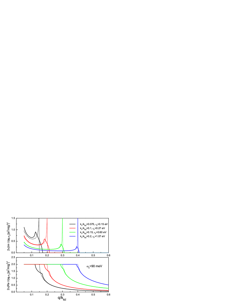
Figure 1: (color online) The imaginary and real parts of the normalized polarization operator $2\pi\left|\Pi(\mathbf{q},\omega=\omega_{0})\right|a^{2}/m\left|g^{0}\right|^{2}$ as a function of the reduced wavevector $q/k_{BZ}$, for different fillings $k_{F}/k_{BZ}$. Solid lines represent the exact results, and the dashed lines the approximate solution (Eq. 17). The four different sets correspond, from left to right, to four increasing values of $k_{F}/k_{BZ}$.

II Phonon renormalization in 2D systems

First let us consider the approximate polarization operator from Eq. 17. Then

$$\omega_{\mathbf{q}}^{app}=\omega_{0}\sqrt{1-2\zeta\left[1-\theta(q-2k_{F})\sqrt{1-(2k_{F}/q)^{2}}\right]}$$ (21)

and according to Eqs. 12 and 17

$$\Gamma_{\mathbf{q}}^{app}=\frac{m\left|g^{0}\right|^{2}}{2\pi a^{2}MV_{F}q}\frac{\theta(2k_{F}-q)}{\sqrt{1-(q/2k_{F})^{2}}}=\frac{\zeta\omega_{0}^{2}}{4\varepsilon_{F}}\frac{\theta(1-Q)}{Q\sqrt{1-Q^{2}}},$$ (22)

where we have introduced, following Ref. froeh , an auxiliary coupling constant $\zeta=N(0)\left|g^{0}\right|^{2}/M\omega_{0}^{2}$ (some authors use another dimensionless constant $\lambda_{0}=2\zeta$). $\Omega_{\mathbf{q}}=\omega_{\mathbf{q}}^{app}+i\Gamma_{\mathbf{q}}^{app}$ gives the renormalized frequency and the damping (see Eqs. 11,12). For $q\leq 2k_{F}$

$$\frac{\Gamma_{\mathbf{q}}^{app}}{\omega_{\mathbf{q}}^{app}}=\frac{\varsigma\omega_{0}}{4\varepsilon_{F}\sqrt{1-2\zeta}}\frac{1}{Q\sqrt{1-Q^{2}}}.$$ (23)

This expression diverges in the limits $Q\rightarrow 0$ and $Q\rightarrow 1.$

Turning now to the exact Eq. 15, we observe that in the small $q$ limit the polarization operator becomes real:

$$\Pi(\mathbf{q}\rightarrow 0,\omega)=-\frac{m\left|g^{0}\right|^{2}}{2\pi a^{2}}\left(\frac{4\varepsilon_{F}}{\omega}\right)^{2}Q^{2}.$$ (24)

Solving the equation

$$D^{-1}(\mathbf{q\rightarrow}0,\omega)=\omega^{2}-\omega_{0}^{2}+\zeta\omega_{0}^{2}\left(\frac{4\varepsilon_{F}}{\omega}\right)^{2}Q^{2}=0$$

one gets

$$\omega_{\mathbf{q\rightarrow}0}=\sqrt{\sqrt{\frac{\omega_{0}^{4}}{4}-16\zeta\omega_{0}^{2}\varepsilon_{F}^{2}Q^{2}}+\frac{\omega_{0}^{2}}{2}}.$$

We choose the branch of the complex square root that gives $\omega_{\mathbf{q\rightarrow}0}\rightarrow\omega_{0}$ for $\zeta\rightarrow 0.$ This means that up to $O(Q^{2})$ there is no damping for the phonon. The phonon spectral function $F(\omega)=-\frac{1}{\pi}{\rm Im}D(\mathbf{q}\rightarrow 0,\omega)$ shows a narrow peak at this frequency and $\Gamma_{\mathbf{q\rightarrow}0}/\omega_{\mathbf{q\rightarrow}0}$ vanishes. The situation at $Q\rightarrow 1$ is similar. In the lowest order in $\omega/\varepsilon_{F}$ we have

$$\Pi(q\mathbf{\rightarrow}2k_{F},\omega)=-\frac{m\left|g^{0}\right|^{2}}{\pi a^{2}}\left[1-(1+i)\sqrt{\omega/8\varepsilon_{F}}\right]$$

This leads to

$$\omega_{2k_{F}} \simeq \omega_{0}\sqrt{1-2\zeta},$$

$$\Gamma_{2k_{F}} = \frac{\zeta\omega_{0}^{2}}{\omega_{2k_{F}}}\sqrt{\frac{\omega_{2k_{F}}}{8\varepsilon_{F}}},$$

and

$$\frac{\Gamma_{2k_{F}}}{\omega_{2k_{F}}}=\frac{\zeta}{1-2\zeta}\sqrt{\frac{\omega_{0}\sqrt{1-2\zeta}}{8\varepsilon_{F}}}$$ (25)

This ratio remains finite in the limit $Q\rightarrow 1,$ although the approximate expression of Eq. 23 diverges for any system with a cylindrical Fermi surface . The main point is that in both cases the well known popular formula

$$\frac{\Gamma_{\mathbf{q}}}{\omega_{\mathbf{q}}} = \frac{\left|g_{0}^{2}\right|}{M}\sum_{\mathbf{k}}\delta(\varepsilon_{\mathbf{k}})\delta(\varepsilon_{\mathbf{k+q}})$$

$$= \frac{\left|g_{0}^{2}\right|}{M(2\pi a)^{2}}\int\frac{dk}{\left|\mathbf{v}(\mathbf{k})\times\mathbf{v}(\mathbf{k}+\mathbf{q})\right|}$$

is not valid near the Kohn singularity.

The results for the linewidth $\Gamma_{\mathbf{q}}$ and the renormalized phonon frequency $\omega_{\mathbf{q}}$ obtained by using the approximate polarization operator as functions of the reduced wavevector $Q=q/2k_{F}$ are shown in Fig.2 by red lines. Parameters are following : the bare phonon frequency $\omega_{0}=90$ meV , the bare constant of EPI $\ \zeta=1/4$.The ratio $k_{F}/k_{BZ}$ is equal to 0.17. It corresponds to $\varepsilon_{F}=0.2$ eV.

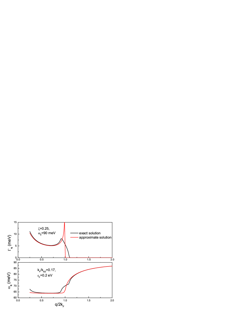
Figure 2: (color online) The linewidth $\Gamma_{\mathbf{q}}$ and the renormalized phonon frequency $\omega_{\mathbf{q}}$ obtained by using the approximation of Eq. 17 and the exact expression Eq. 15, for the following parameters : the bare phonon frequency $\omega_{0}=90$ meV , the bare constant of EPI $\ \zeta=1/4$. The filling corresponds to $k_{F}/k_{BZ}=0.17$ and $\varepsilon_{F}=0.2$ eV.

The approximate result agrees with that of Ref.an (their Fig.4). The exact result (black lines) has been obtained by a numerical solution of Eqs. 8,9 using the polarization operator from the Eq. 15. The latter, in contrast to the approximate expression, shows two shoulders in the wavevector dependence of the renormalized frequency $\omega_{\mathbf{q}}$ (see also $\left|\mathrm{Re}\Pi(\mathbf{q},\omega_{0})\right|$ in the bottom panel of Fig. 2). The first one corresponds to the maximum of $\left|\mathrm{Im}\Pi(\mathbf{q},\omega)\right|$ (or $\Gamma_{\mathbf{q}}$) and the second one to vanishing of these values.

III Electron self-energy

The electron self-energy is expressed via the electron and phonon Green functions:

$$\Sigma(p)=ig^{0}\int G(p-k)D(k)\Gamma(p,p-k,k)\frac{d^{D+1}k}{(2\pi)^{D+1}},$$

where $p=\{\mathbf{p},\varepsilon\}$. It was shown by Migdal migdal that one can neglect the vertex corrections $\Gamma(p,p-k,k)\simeq g^{0}(1+\sqrt{m/M})$ and that the function $G(\varepsilon,\mathbf{k})$ differs from the bare electron Green function (Eq. 7) only in the narrow interval of momenta $\left|k-k_{F}\right|\lesssim\omega_{ph}/V_{F}$ and frequencies $\left|\omega\right|\lesssim\omega_{ph}.$ Thus, the full electron Green function $G(p)$ can be substituted by the corresponding function for noninteracting electrons (Eq. 7). Using the Eq. 3, the electron self-energy for $T=0$ becomes (see, e.g., Refs.mahan , am )

$$\Sigma(\mathbf{k},\omega)=\sum_{\mathbf{q}}\delta(\varepsilon_{\mathbf{k+q}})\frac{\left|g^{0}\right|^{2}}{2M\omega_{\mathbf{q}}}\int d\xi\left[\frac{\theta(\xi)}{\omega-\xi-\omega_{\mathbf{q}}+i\Gamma_{\mathbf{q}}}+\frac{\theta(-\xi)}{\omega-\xi+\omega_{\mathbf{q}}-i\Gamma_{\mathbf{q}}}\right].$$

This is a trivial generalization of the standard expressions onto the finite phonon linewidth case. Let us average the self energy over the Fermi surface

$$\Sigma(\omega) = \frac{1}{N(0)}\sum_{\mathbf{k}}\delta(\varepsilon_{\mathbf{k}})\Sigma(\mathbf{k},\omega)$$

$$= -\frac{1}{N(0)M}\sum_{\mathbf{k}}\sum_{\mathbf{q}}\delta(\varepsilon_{\mathbf{k}})\delta(\varepsilon_{\mathbf{k+q}})\frac{\left|g^{0}\right|^{2}}{4\omega_{\mathbf{q}}}\left\{\ln\frac{\Gamma_{\mathbf{q}}^{2}+(\omega_{\mathbf{q}}-\omega)^{2}}{\Gamma_{\mathbf{q}}^{2}+(\omega_{\mathbf{q}}+\omega)^{2}}+2i\left[\tan^{-1}\left(\frac{\omega_{\mathbf{q}}-\omega}{\Gamma_{\mathbf{q}}}\right)-\tan^{-1}\left(\frac{\omega_{\mathbf{q}}+\omega}{\Gamma_{\mathbf{q}}}\right)\right]\right\}.$$

The limit $\lambda=-\lim_{\omega\rightarrow 0}\mathrm{Re}\Sigma(\omega)/\omega$ is nothing but the standard electron-phonon coupling constant

$$\lambda_{\Gamma}=\frac{1}{MN(0)}\sum_{\mathbf{k}}\sum_{\mathbf{q}}\delta(\varepsilon_{\mathbf{k}})\left|g^{0}\right|^{2}\delta(\varepsilon_{\mathbf{k+q}})\frac{1}{\Gamma_{\mathbf{q}}^{2}+\omega_{\mathbf{q}}^{2}}=\sum_{\mathbf{q}}\tilde{N}_{\mathbf{q}}(0)\frac{\left|g^{0}\right|^{2}}{M}\frac{1}{\Gamma_{\mathbf{q}}^{2}+\omega_{\mathbf{q}}^{2}},$$ (27)

where we introduced the phase space function (sometimes called “nesting function”)

$$\tilde{N}_{\mathbf{q}}(0)=\frac{1}{N(0)}\sum_{\mathbf{k}}\delta(\varepsilon_{\mathbf{k}})\delta(\varepsilon_{\mathbf{k+q}}).$$ (28)

For a 2D cylindrical Fermi surface we have

$$\tilde{N}_{\mathbf{q}}(0)=\frac{\theta(1-Q)}{4\pi\varepsilon_{F}Q\sqrt{1-Q^{2}}},$$ (29)

which diverges at $Q\rightarrow 0$ and $Q\rightarrow 1$. Following Ref. allen we can introduce the “mode $\lambda$” via the expression $\lambda=\sum_{\mathbf{q}}\lambda_{\mathbf{q}}$. Then

$$\lambda_{\mathbf{q}}=\tilde{N}_{\mathbf{q}}(0)\frac{\left|g^{0}\right|^{2}}{M}\frac{1}{\Gamma_{\mathbf{q}}^{2}+\omega_{\mathbf{q}}^{2}}.$$

In the weak-damping approximation for we recover the standard formula

$$\lambda_{\mathbf{q}}^{app}=\tilde{N}_{\mathbf{q}}(0)\frac{\left|g^{0}\right|^{2}}{M}/\omega_{\mathbf{q}}^{2},$$ (30)

but for $\Gamma_{\mathbf{q}}\gg\omega_{\mathbf{q}}$ the contribution of strongly damped phonons to total $\lambda_{\mathbf{q}}$ is suppressed.

The result (27) we can get also if we introduce, according to Eq. 3, a generalized Eliashberg function

$$\alpha_{\Gamma}^{2}(\omega)F(\omega) = \frac{1}{2\pi MN(0)}\sum_{\mathbf{k,q}}\frac{\delta(\varepsilon_{\mathbf{k}})\left|g^{0}\right|^{2}\delta(\varepsilon_{\mathbf{k+q}})}{2\omega_{\mathbf{q}}}\frac{1}{2}\left[\frac{\Gamma_{\mathbf{q}}}{(\omega-\omega_{\mathbf{q}})^{2}+\Gamma_{\mathbf{q}}^{2}}-\frac{\Gamma_{\mathbf{q}}}{(\omega+\omega_{\mathbf{q}})^{2}+\Gamma_{\mathbf{q}}^{2}}\right]=$$ (31)

$$\frac{1}{2\pi M}\sum_{\mathbf{q}}\frac{\tilde{N}_{\mathbf{q}}(0)\left|g^{0}\right|^{2}}{2\omega_{\mathbf{q}}}\frac{1}{2}\left[\frac{\Gamma_{\mathbf{q}}}{(\omega-\omega_{\mathbf{q}})^{2}+\Gamma_{\mathbf{q}}^{2}}-\frac{\Gamma_{\mathbf{q}}}{(\omega+\omega_{\mathbf{q}})^{2}+\Gamma_{\mathbf{q}}^{2}}\right].$$

The second term in this expression cancels out the nonphysical behavior at low and high frequencies. Otherwise $\lambda_{\Gamma}$ would have be divergent. Eqs. 27,31 are general and valid for not only for the 2D systems, where phase space factor (Eq. 28) is divergent.

For $\Gamma_{\mathbf{q}}\ll\omega_{\mathbf{q}}$ we have

$$\alpha_{app}^{2}(\omega)F(\omega)=\frac{1}{N(0)M}\sum_{\mathbf{k,q}}\frac{\delta(\varepsilon_{\mathbf{k}})\left|g^{0}\right|^{2}\delta(\varepsilon_{\mathbf{k+q}})}{2\omega_{\mathbf{q}}}\delta(\omega-\omega_{\mathbf{q}})=\frac{1}{2\pi N(0)}\sum_{\mathbf{q}}\frac{\Gamma_{\mathbf{q}}^{app}}{\omega_{\mathbf{q}}}\delta(\omega-\omega_{\mathbf{q}}),$$ (32)

where in the last equality we have used the approximate Eq. 12. Note that the Eq. 32 is a consequence of that fact that the damping $\Gamma_{\mathbf{q}}^{app}$, according to Eq. 12, can be expressed via the “nesting function” (Eq. 28) and both are determined by the same function ${\rm Im}\Pi^{\prime}(q,0)\equiv d{\rm Im}\Pi(q,\omega)/d\omega|_{\omega=0}$. In a general case these functions can be different. This result without using the pole approximation for the phonon Green function can be trivially obtained in the Matsubara formalism. In this case it one does not need to solve the Dyson equation. In the lowest order in coupling for $T=0$ the self-energy has a form

$$\Sigma(i\varepsilon,\mathbf{k})=-i\int\frac{d(i\omega)}{2\pi}\sum_{\mathbf{k}^{\prime},\nu}\left|g^{0}\right|^{2}D_{M\nu}(i\omega+i\varepsilon,\mathbf{k,k}^{\prime})\frac{1}{i\omega-\varepsilon_{\mathbf{k}^{\prime}}-\Sigma(i\omega,\mathbf{k}^{\prime})},$$

where

$$D_{M\nu}(i\omega,\mathbf{k,k}^{\prime})=(1/\pi)\int_{0}^{\infty}d\Omega\mathrm{Im}D(\Omega+i\delta,\mathbf{k,k}^{\prime})\left[\left(i\omega-\Omega\right)^{-1}-\left(i\omega+\Omega\right)^{-1}\right].$$ (33)

We can also average the self-energy over the Fermi surface $\Sigma(i\varepsilon)=\sum_{\mathbf{k}}\delta(\varepsilon_{\mathbf{k}})\Sigma(i\varepsilon,\mathbf{k})/N(0).$

$$\Sigma(i\varepsilon)=\frac{1}{N(0)}\sum_{\mathbf{k}}\sum_{\mathbf{q}}\delta(\varepsilon_{\mathbf{k}})\left|g^{0}\right|^{2}\delta(\varepsilon_{\mathbf{k+q}})\int_{-\infty}^{\infty}\frac{d\omega}{2\pi}D_{M}(\mathbf{q},i\omega)\int_{-\infty}^{\infty}\frac{d\xi}{i(\varepsilon-\omega)-\xi}$$

The integral $\int_{-\infty}^{\infty}\frac{d\xi}{i(\varepsilon-\omega)-\xi}=-i2\pi\mathrm{sign}(\varepsilon-\omega)$ allows to calculate the physical coupling constant $\lambda$

$$\lambda = -\frac{\partial\Sigma_{el}(i\varepsilon)}{\partial i\varepsilon}|_{\varepsilon\rightarrow 0}=-\lim_{\varepsilon\rightarrow 0}\frac{1}{N(0)}\sum_{\mathbf{k}}\sum_{\mathbf{q}}\delta(\varepsilon_{\mathbf{k}})\left|g^{0}\right|^{2}\delta(\varepsilon_{\mathbf{k+q}})\int\frac{d\omega}{2\pi}D(\mathbf{q},i\omega)2\pi\delta(\varepsilon-\omega)$$

$$= -\frac{1}{N(0)}\sum_{\mathbf{k}}\sum_{\mathbf{q}}\delta(\varepsilon_{\mathbf{k}})\left|g^{0}\right|^{2}\delta(\varepsilon_{\mathbf{k+q}})D_{M}(\mathbf{q},i0)=-\frac{1}{N(0)}\sum_{\mathbf{k}}\sum_{\mathbf{q}}\delta(\varepsilon_{\mathbf{k}})\left|g^{0}\right|^{2}\delta(\varepsilon_{\mathbf{k+q}})\frac{1}{D_{M0}^{-1}(i0)-\Pi_{M}(\mathbf{q},i0)}.$$

On the Matsubara axes, for 2D system, according to Eq. 20, the phase space factor vanishes for $q>2k_{F}$ and $\Pi_{M}(q\leq 2k_{F},i0)=-2\zeta\omega_{0}^{2}$ is a constant (see Eqs.20 and 19). Using Eqs. 2,33 we get $D_{M0}^{-1}(i0)=-M\omega_{0}^{2}$ and

$$\lambda=\zeta/(1-2\zeta).$$ (34)

In a 3D case $\Pi_{M}(\mathbf{q},i0)$ is a rather complicated function of $q$ and the Eq. 34 is only an approximation (as was probably firstly mentioned by Fröhlich froeh ). The physical meanings of the coupling constants $\lambda$ and $\zeta$ that they are measures of the renormalization of the phonon frequency from $\omega_{0}$ to $\omega_{\mathbf{q}}$ (cf. a discussion for 3D systems in Ref.maks ).

Turning back to the 2D case, according to Eq. 27 we can neglect all divergent contributions near $Q=0$ and $Q=1$. Elsewhere we can use Eq. 30.

One should keep in mind that the conventional coupling constant is $\lambda=\zeta/(1-2\zeta)$. This parameter determines electronic properties (Fermi velocities, $T_{c}$, etc.). The other parameter, $\zeta=\lambda/(1+2\lambda)<1/2$, defines the observable phonon frequency, $\omega_{\mathbf{q}}=\omega_{0}\sqrt{1-2\zeta}$.

IV Conclusions

First of all, the standard well-known expression

$$\alpha^{2}(\omega)F(\omega)=\frac{1}{2\pi N(0)}\sum_{\mathbf{q}}\frac{\Gamma_{\mathbf{q}}}{\omega_{\mathbf{q}}}\delta(\omega-\omega_{\mathbf{q}})$$

$$\equiv \frac{1}{N(0)M}\sum_{\mathbf{k}}\sum_{\mathbf{q}}\frac{\delta(\varepsilon_{\mathbf{k}})\left|g^{0}\right|^{2}\delta(\varepsilon_{\mathbf{k+q}})}{2\omega_{\mathbf{q}}}\delta(\omega-\omega_{\mathbf{q}}),$$

is valid only in the lowest order in the “bare” phonon linewidth, $\Gamma_{\mathbf{q}}$, which is not an acceptable approximation in case of strong Kohn singularities, and particularly for a cylindrical Fermi surface. $\Gamma_{\mathbf{q}}$ in this approximation is not the actual phonon line width; as opposed to $\Gamma_{\mathbf{q}},$ determined by the oversimplified Eq. 12, the real phonon linewidth does not diverge even for an ideally cylindrical Fermi surface. Second, the renormalized $\lambda$ for a cylindrical Fermi surface and parabolic bands does not depend on filling.

References

• (1) I.I. Mazin and V.P. Antropov, Physica C385, 49 (2003).
• (2) Y. Kong, O. V. Dolgov, O. Jepsen and O. K. Andersen, Phys. Rev. B64, 020501(R) (2001).
• (3) A.Y. Liu, I. I. Mazin and J. Kortus, Phys. Rev. Let. 87, 087005 (2001).
• (4) J.M. An, S.Y. Savrasov, H. Rosner, and W.E. Pickett, Phys. Rev. B 66, 220502(R) (2002); W.E. Pickett, J.M. An,  H. Rosner, and S.Y. Savrasov, Physica C 387, 117 (2003)
• (5) A.Y. Liu, I. I. Mazin. Phys. Rev. B75, 064510 (2007); M. Calandra, A.N. Kolmogorov, and S. Curtarolo, Phys. Rev B75, 144506 (2007).
• (6) In publications one can sometimes find the phonon Green functions which differ from ours in some factors. This ambiguity can be traced down to the definitions of the phonon field operators (Eq. 1). In this case the corresponding factors appear in the electron-ion matrix element (Eq. 6). But all physical quantities as EPI coupling constant, Eliashberg functions etc. are determined by the unique combination $\left|g^{0}\right|^{2}D$ that is independent on definitions.
• (7) A.B. Migdal, Sov. Phys.-JETP, 7, 996 (1958)
• (8) P.B. Allen in : Dynamical properties of solids, eds. G.K. Horton and A.A. Maradudin, v. 3, ( North Holland, 1980), p. 157.
• (9) P.B. Allen, Phys. Rev. B 6, 2577 (1972)
• (10) M. Calandra, and F. Maury, Phys. Rev. B 71, 064501 (2005)
• (11) F. Stern, Phys. Rev. Letts., 18, 546 (1967)
• (12) T. Ando, A.B. Fowler, and F. Stern, Rev. Mod. Phys., 54, 445 (1982)
• (13) Y. Zhang, V.M. Yakovenko, and S. Das Sarma, Phys. Rev. B71,115105 (2005)
• (14) A. Isihara and T. Toyoda, Z. Phys. B23, 389 (1976); A. Isichara, in Solid State Physics, ed. by H. Erenreich, F. Zeitz, and D. Turnbull, (Academic, N.Y., 1989), v. 42, p.271
• (15) H. Fröhlich, Phys. Rev. 79, 845 (1950)
• (16) G.D. Mahan, Many-Particle Physics, Plenum Press, New York, 1981
• (17) P.B. Allen and B. Mitrović, in Solid State Physics, ed. by H. Erenreich, F. Zeitz, and D. Turnbull, (Academic, N.Y., 1982), v. 37, p.1
• (18) E.G. Maksimov and D.I. Khomskii, in High-Temperature Superconductivity , ed. by V.L. Ginzburg and D.A. Kirzhnits, Consultants Bureau, New York, 1982, Chap. 3.