Modeling the line variations from the wind-wind shock emissions of WR 30a

Abstract

The study of Wolf-Rayet stars plays an important role in evolutionary theories of massive stars. Among these objects, $\sim 20\%$ are known to be in binary systems and can therefore be used for the mass determination of these stars. Most of these systems are not spatially resolved and spectral lines can be used to constrain the orbital parameters. However, part of the emission may originate in the interaction zone between the stellar winds, modifying the line profiles and thus challenging us to use different models to interpret them. In this work, we analyzed the HeII$\lambda$4686Å + CIV$\lambda$4658Å blended lines of WR30a (WO4+O5) assuming that part of the emission originate in the wind-wind interaction zone. In fact, this line presents a quiescent base profile, attributed to the WO wind, and a superposed excess, which varies with the orbital phase along the 4.6 day period. Under these assumptions, we were able to fit the excess spectral line profile and central velocity for all phases, except for the longest wavelengths, where a spectral line with constant velocity seems to be present. The fit parameters provide the eccentricity and inclination of the binary orbit, from which it is possible to constrain the stellar masses.

1 Introduction

Massive stars are known to drive strong winds, which are responsible for the transfer of a large amount of the stellar mass to the interstellar medium, contributing to the feedback of chemical elements, and to the creation of cloud cavities in which these objects are found. Typically, O stars present mass-loss rates of $\dot{M}_{\rm O}\sim 10^{-6}-10^{-5}$ M_⊙ yr^-1 and wind velocities of $v_{\rm O}\sim 2000-3500$ km s^-1, while Wolf-Rayet (WR) stars present $\dot{M}_{\rm WR}\sim 10^{-6}-10^{-4}$ M_⊙ yr^-1 and $v_{\rm WR}\sim 1000-4000$ km s^-1 (Nugis & Lamers 2000, Lamers 2001).

In massive binary systems in which both stars present high mass-loss rates and high-velocity winds, the collision of the winds will occur. Therefore, a contact surface is formed where the momenta of the two winds are equal, surrounded by two shocks. The post-shocked gas, cools as it flows along the contact surface and is responsible for strong free-free emission at X-ray and radio wavelengths. X-rays in massive binary systems are orders of magnitude higher than those observed in single massive stars, and are used as an indication of binarity.

UV and optical lines can also indicate the binary nature of a given object, when they present periodic profile variations. If the lines are of photospheric or atmospheric origin, as the stars move along their orbit, they suffer Doppler shifts, which depend on the orbital phase and inclination. However, some massive objects show periodic variable line profiles that cannot be explained under these assumptions.

Seggewiss (1974) noted that the binary system WR79 presented two peaks, superimposed to the CIII emission line, which changed their position and intensity with time. Typically, in double line spectroscopic binaries, each peak moves in a different direction, indicating opposite velocity components along the line of sight for each star; however in WR79 both peaks moved in the same direction. L$\rm\ddot{u}$hrs (1997) presented a model in which the two peaks were not produced by the stellar photosphere, but were generated by the flowing gas at the contact surface between the two strong shocks. This model reproduced well the data for WR 79, but failed to reproduce the line profiles of other WR binary systems, among them WR 30a (Bartzakos, Moffat & Niemela 2001). Falceta-Gonçalves, Abraham & Jatenco-Pereira (2006) improved L$\rm\ddot{u}$hrs’ model introducing more realistic parameters, as stream turbulence and gas opacity, to account for the line broadening and peak displacement.

In the present work, we applied this model to WR 30a, which was classified as a WO4+O5 binary system (Moffat & Seggewiss 1984, Crowther et al. 1998); its binary nature was reported by Niemela (1995) based on spectral-line radial velocities obtained with a high temporal resolution. Later, Gosset et al. (2001) presented a detailed analysis of the spectra of WR30a for several epochs and were able to confirm the binary hypothesis and to determine the period of $P\sim 4.6$ days. They also noted strong line-profile variations, which made more difficult the determination of the stellar mass ratio and the orbital inclination from standard methods. They concluded that the CIV$\lambda$4658Å line-profile variations were related to wind-wind collision processes, but did not model the lines under such an assumption. The same conclusion was reached by Bartzakos, Moffat & Niemela (2001) using the CIV$\lambda$5801Å line. Also, Paardekooper et al. (2003) presented photometric measurements at $V$ and $B$ bands; the light curves confirmed the period obtained by Gosset et al. (2001), but also showed higher frequency variability in the $V$ band, with timescale of hours. They concluded that this could be due to the strong variability of the CIV$\lambda$5801Å line, possibly related to the wind-wind interaction.

In the present work, we tested the wind-wind shock emission hypothesis on the CIV$\lambda$4658 Å excess line profile variations measured by Gosset et al. (2001) using the model developed by Falceta-Gonçalves, Abraham & Jatenco-Pereira (2006), which is briefly described in Section 2. In Section 3, we show the results obtained for WR 30a and present a brief discussion, followed by the conclusions in Section 4.

2 Wind-wind emission model

In the proposed situation, in which both stars present high mass-loss rates in supersonic winds, the contact surface, which is schematically shown in Figure 1, will have a geometry described analytically by (Luo, McCray & Mac-Low 1990):

$$\vskip 6.0pt plus 2.0pt minus 2.0pt\frac{dy}{dz}=\frac{(\eta^{-1/2}{d_{2}}^{2}+{d_{1}}^{2})y}{\eta^{-1/2}{d_{2}}^{2}z+{d_{1}}^{2}(z-D)},\vskip 6.0pt plus 2.0pt minus 2.0pt$$ (1)

where $D$ is the distance between the stars; $d_{1}$ and $d_{2}$ are the distances of the primary and secondary stars to the contact surface, respectively, and $\eta=\dot{M_{s}}v_{s}/\dot{M_{p}}v_{p}$, where $\dot{M_{p}}$ and $\dot{M_{s}}$ are the mass-loss rates of the primary and the secondary stars, and $v_{p}$ and $v_{s}$ their respective wind velocities. The contact surface will asymptotically have a conical shape with an opening angle defined by $\beta$, given by:

$$\vskip 6.0pt plus 2.0pt minus 2.0pt\beta\simeq 120^{\circ}\left(1-\frac{\eta^{2/5}}{4}\right)\eta^{1/3},\vskip 6.0pt plus 2.0pt minus 2.0pt$$ (2)

and the apex will occur at a distance to the primary star given by:

$$\vskip 6.0pt plus 2.0pt minus 2.0ptd_{1}|_{\rm apex}=D/(1+\eta^{1/2}).\vskip 6.0pt plus 2.0pt minus 2.0pt$$ (3)

Two shock fronts will be formed on both sides of the contact surface, generated by each wind, and the gas in the post-shock region will flow away along the contact surface. While it flows, the gas will cool due to expansion and radiation. This emission, detectable from radio wavelengths to X-rays, is the signature of wind-wind collisions (Usov 1992, Falceta-Gonçalves, Jatenco-Pereira & Abraham 2005, Abraham et al. 2005, Pittard & Dougherty 2006). The stream of hot gas flowing along the contact surface will, eventually, reach temperatures that allow the recombination of certain elements. In this situation, the observer will detect the emission line shifted due to the stream velocity component along the line of sight, which may intercept regions with different velocity components, as shown in Figure 1. The shaded regions in the shock layer represent the emitting fluid elements. Here, observer $A$ would detect two emission lines, a blueshifted line from fluid element 1, and a redshifted line from element 2. On the other hand, observer $B$ would detect two blueshifted lines.

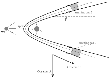
Figure 1: Schematic view of the wind-wind interaction surface and the model geometry.

L$\rm\ddot{u}$hrs (1997) used these concepts to model line-profile variability during the orbital period of WR79. To reproduce the observations, he assumed a large emission region, limited by two cones with aperture angles $\beta$ and $\beta+\Delta\beta$, selected $ad$ $hoc$ to fit the the observations. However, the assumption is valid only in the case of quasi-adiabatic shocks, which occur in long-period systems. Radiative shocks evolve much faster, creating layers that are narrow and turbulent (Stevens, Blondin & Pollock 1992), and therefore cannot simply be described by a fixed range of beta values as assumed by L$\rm\ddot{u}$hrs (1997). Falceta-Gonçalves, Abraham & Jatenco-Pereira (2006) by-passed this problem by including turbulence in the stream layer, and also took into account the shocked gas opacity, which may result in line profile asymmetries. In that work, the line profile is obtained by integrating the emission intensities of each fluid element as:

$$\vskip 6.0pt plus 2.0pt minus 2.0ptI(v)=\mathcal{C(\varphi)}\int_{0}^{\pi}\exp\left[-\frac{\left(v-v_{\rm obs}\right)^{2}}{2\sigma^{2}}\right]e^{-\tau(\alpha)}d\alpha,\vskip 6.0pt plus 2.0pt minus 2.0pt$$ (4)

where:

$$\vskip 6.0pt plus 2.0pt minus 2.0ptv_{\rm obs}=v_{\rm flow}(-\cos\beta\cos\varphi\sin i+\sin\beta\cos\alpha\sin\varphi\sin i$$

$$-\sin\beta\sin\alpha\cos i),\vskip 6.0pt plus 2.0pt minus 2.0pt$$ (5)

is the observed stream velocity component projected into the line of sight, $\alpha$ is the azimuthal angle of the shock cone, $i$ is the orbital inclination, $\varphi$ is the orbital phase angle, $\sigma$ is the turbulent velocity amplitude, $\tau$ is the optical depth along the line of sight and $\mathcal{C(\varphi)}$ is a normalization constant.

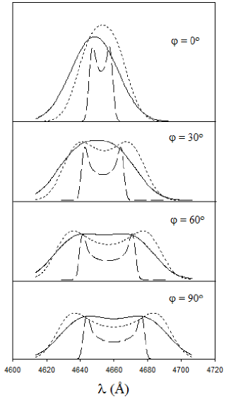
Figure 2: Synthetic line profiles for models (a): $\beta=55\degr$, $i=60\degr$, $\sigma=0.1$ and $v_{\rm flow}=1000$ km s^-1 (dashed line) (b): $\beta=55\degr$, $i=60\degr$, $\sigma=0.5$ and $v_{\rm flow}=1500$ km s^-1 (solid line) and (c): $\beta=70\degr$, $i=60\degr$, $\sigma=0.3$ and $v_{\rm flow}=1000$ km s^-1 (dotted line); for different orbital phases ranging from $\varphi=0\degr$ to $90\degr$.

In Figure 2, we show the model results for different orbital and stream parameters. The dashed line model (a) was calculated using $\beta=55^{\circ}$, $i=60^{\circ}$, $\sigma=0.1$ and $v_{\rm flow}=1000$ km s^-1; the solid line (b) using $\beta=55^{\circ}$, $i=60^{\circ}$, $\sigma=0.5$ and $v_{\rm flow}=1500$ km s^-1; and the dotted line (c) using $\beta=70^{\circ}$, $i=60^{\circ}$, $\sigma=0.3$ and $v_{\rm flow}=1000$ km s^-1. It is noticeable that, e.g. in models (a) and (c), there are two peaks generated by each of the shock-cone layers intercepted by the line of sight. As shown by Falceta-Gonçalves et al. (2006), this is valid for $0\degr\leq i<90\degr$, while for $i=90^{\circ}$, the profile will present a single peak at $\varphi=0\degr$, which corresponds to the cone axis coincident with the line of sight. Another comparative analysis between (a) and (c) shows the effect of changing $\beta$; as $\beta$ increases, the distance between the two peaks becomes larger. Models (b) and (c) present high turbulence amplitude, which leads to a larger line broadening. Here, we neglected the gas opacity (i.e. $\tau<<1$) to show the presence of two peaks in the line profiles. If the shock cone is optically thick, part of the emission along the line of sight will be absorbed, and the redder peak will be less intense or, eventually, completely disappear.

In the next section we present the application of this model to the CIV$\lambda$4658Å excess line-profiles of WR30a, in order to determine the orbital and stellar parameters.

3 The case of WR30a

Gosset et al. (2001) presented a detailed spectroscopic study of WR30a with data covering 30 days, which corresponds to about 6 complete orbital cycles. From their observations, the strongest broad emission line is identified as a blend dominated by CIV$\lambda$4658Å and HeII$\lambda$4686Å. Subtracting a constant parabolic base line, attributed to the WR stellar wind emission, they obtained the averaged residual spectra shown in Figure 3. This excess emission presents anomalous profiles and variability in both line intensity and central wavelenght, all related to the orbital phase. This effect could originate in selective wind eclipses, resulting in different profiles as the O-star is located behind or in front of the WR star along the orbital motion. However, this is not the case in WR30a because due to its low orbital inclination no phase-dependent atmospheric absorption would be expected.

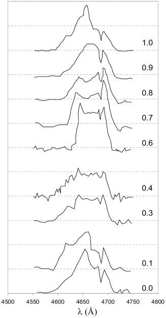
Figure 3: Excess emission line profiles obtained from Gosset $et$ $al.$ (2001).

3.1 The orbital parameters

As it is clear from Figure 2, a wind-wind interaction model is compatible with the line profiles observed in WR30a. Hence, we applied the model described in the previous section to determine the binary-system parameters. An important model parameter in equation (4) is the optical depth $\tau(\alpha)$ of the absorbing material; Falceta-Gonçalves et al. (2006) assumed that it is the absorption by the dense material that accumulates along the contact surface that produces the asymmetries in the line profiles, while any other absorption is taken into account by the multiplying factor $C(\varphi)$. Since most of the lines seem to be symmetric, at least within the uncertainties due to the subtraction of a phase independent base profile, we assumed $\tau(\alpha)=0$. It turned out from our fitting that $C(\varphi)$ is also independent of the orbital phase..

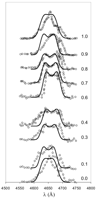
Figure 4: Best fitting synthetic line profiles obtained for $\beta=50^{\circ}$, $i=20^{\circ}$, $\sigma=0.3$ and $v_{flow}=2200$km s^-1. The orbital phase of each data set is exactly the same shown in Figure 2.

In order to model the observed excess emission spectra for each orbital phase, we performed calculations varying the opening angle, the turbulence amplitude and the stream velocity for different values of the orbital inclination. We were not able to fit simultaneously the complete width of the observed profiles and their mean velocities for all epochs, even for high values of the orbital inclination. Instead, we obtained a better agreement when we considered that the emission at the longest wavelengths, seen as a peak near 4690Å  is not formed in the shock region. The best fit occurred for $\beta=50^{\circ}\pm 5\degr$, $i=20^{\circ}\pm 5\degr$, $v_{\rm flow}=2200\pm 500$ km s^-1, and $\sigma=0.3\pm 0.1$; the corresponding profiles are shown in Figure 4. The phase angles used for the fit for each epoch, and their respective uncertainties are shown in Figure 5, as a function of the orbital phase. The uncertainties in the parameters were obtained by changing each one of them independently until the model became incompatible with the observations. The excess profile for orbital phase 0.7 is very well-fitted by the wind-wind emission model, with the exception of the already mentioned additional peak near 4690Å. For orbital phases near 1.0 the model profiles are wider than those observed, which seemed to be single peaked. This may be related to the subtracted base line profile, which was obtained by Gosset et al. (2001) for phase 0.55 and equally applied to all orbital phases.

If the subtracted profile is produced in the WR stellar wind, as it seems to be the case, it would be necessary to take into account the fact that the wind is not completely symmetric but shaped by the conic hole with aperture $\beta$, as the wind is deflected at the shock. Since the orientation of this hole changes with orbital phase, we would expect also changes in the broad profile produced by the WR wind. For the particular case of $i=90^{\circ}$, when the WR star is in conjunction regarding the observer, there will be a stronger deficit of emission at the redshifted part of the line profile. On the other hand, if the WR star is in opposition, the amount of upcoming gas will be lower, affecting more the blueshifted emission. For $i=0^{\circ}$, the profile would not change as the orientation of the cone is always the same with respect to the observer. For WR30a, with $i\simeq 20^{\circ}$, at WR conjunction there will be mainly an effect on the red side of the profile but the blues side would also be affected. The opposite would occur at WR opposition. This is compatible with the narrower excess profiles near phase 1.0 as can be seen in Figure 4.

At long wavelengths, the excess near 4690Å could possibly be the blended emission from the HeII$\lambda$4686Å line; although it seems decoupled from the shock emission during the orbital period, it is too narrow $\sim 20$Å (1300 km s^-1) to be attributed to the WR stellar wind ($>2000$km s^-1). It could be, however, a fraction of the WR P-Cygni profile or it could also be related to the remnant shocked material surrounding the stellar system, ionized by the stellar radiation. Gosset et al. (2001) also attributed the narrow absorption superposed on the broad excess emission to a HeII$\lambda$4686Å absorption line from the O star.

The phase angles derived from our model provide additional information regarding the orbit, namely its eccentricity, since the model strictly depends on the angle between the cone axis and the line of the sight, while the observed profiles depend on the orbital phase. The dependence between the two parameters is related to the orbital eccentricity, as shown in Figure 5 for $e=0.0,0.2$ and $0.5$. The dotted line represent the result for $e=0.0$ (circular orbit), in which the phase angle changes linearly with time. The dashed line shows the fast phase angle variation during the periastron passage for $e=0.5$. The data for WR30a seem to fit best the curve corresponding to $e=0.2$ when the lines are shifted by $\varphi_{0}=-20^{\circ}$ in phase angle (0.056 of the orbital phase). Part of this shift could by explained by the Coriolis Effect, which produces a deviation of the cone axis as a consequence of the relative motion of the stars; however, Gosset et. al. (2001) estimated this effect as only 0.01 in orbital phase. Most of the contribution is probably produced by the binning of the data in intervals of one tenth of the period, which could also explain why the eccentricity we found is different from zero.

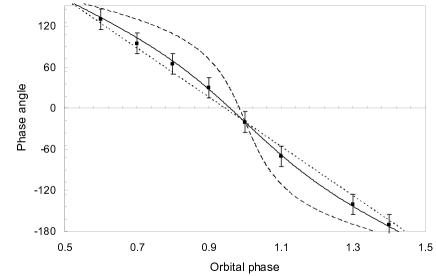
Figure 5: The dependence of the phase angle on the orbital phase for eccentricities e = 0.0 (dotted), 0.2 (solid) and 0.5 (dashed), where $\varphi_{0}=-20^{\circ}$. The data for WR30a (squares) were obtained from the phase angles of the fits and the observed orbital phases of Figure 3.

3.2 The stellar masses

After modeling the wind-wind shock emission, and determining the orbital parameters of the binary system, we can constrain the stellar masses. For this purpose, we analyzed the velocity curve of the O-star obtained by Gosset et al. (2001) from measurements of four lines (HeII$\lambda$4542Å, H$\gamma$, HeII$\lambda$4200Å and H8) during the orbital period. Their results are shown in Figure 6, as well as the fit of the modeled curve for $e=0.2$ and $K_{\rm O}=25$ km s^-1. As a result, the mass function:

$$\vskip 6.0pt plus 2.0pt minus 2.0ptf(m)=\frac{K_{\rm O}^{3}P}{2\pi G}=\frac{(M_{\rm WR}\sin i)^{3}}{(M_{\rm WR}+M_{\rm O})^{2}},\vskip 6.0pt plus 2.0pt minus 2.0pt$$ (6)

gives $f(m)=0.0074$ M_⊙. If we assume $M_{\rm O}=40$ M_⊙ (60 M_⊙), using $i=20\degr$ obtained from the shock emission, we find $M_{\rm WR}=7.5$ M_⊙ (9.7 M_⊙), which gives a mass ratio $M_{\rm WR}/M_{\rm O}\sim 0.2$. Regarding the orbit, using the obtained mass function and orbital inclination, we find $a_{\rm O}\simeq 5.4$ R_⊙ and $a_{\rm WR}\simeq 30$ R_⊙.

These results are in agreement with those expected for the masses of O and WO stars $40-60$ and $8-10$ M_⊙, respectively (Howarth & Prinja 1989, de Marco & Schmutz 1999); also, the distance between the stars is larger than the sum of the expected stellar radii: $D>R_{\rm O}+R_{\rm WR}\sim 20$ R_⊙ (Schaerer, Schmutz & Grenon 1997).

From Equation 2 and the value of the cone-opening angle ($\beta=50^{\circ}$) we calculated the wind momentum ratio and obtained $\eta=0.12$, which is compatible with typical observed values in systems similar to WR30a (Lamers 2001). From Equation 3, we estimated the distance from the apex to the stars: for $\eta=0.12$ and the total separation $D=35.4$ R_⊙ we obtained $d_{1}|_{\rm apex}~{}25$ R_⊙ and $d_{2}|_{\rm apex}~{}10$ R_⊙. Considering a typical O-star, $d_{2}|_{\rm apex}$ would be of the same order than the stellar radius, and the frontal part of its wind could be crushed onto the stellar surface. The shape of the contact surface would be spherical near the apex, affecting maybe the X-ray emission from the system (Usov 1992), but our model will still be valid, since the line emission originates at larger distances from the apex, on the contact surface.

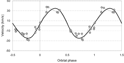
Figure 6: The O-star radial velocity as function of the orbital phase. The observed data (circles) were obtained from Gosset et al. (2001). The solid line represent the fit for $K_{O}=25$ km s^-1 and $e=0.2$.

4 Conclusions

In this work we presented an application of the wind-wind shock emission model proposed by Falceta-Gonçalves et al. (2006) to the line profile variations of WR 30a. In this model, the wind-wind shock structure can be represented by a cone, along which the shocked material flows. This gas will emit radiation, cool down and eventually reach recombination temperatures. The observed emission lines will then suffer Doppler shifts due to the stream velocity component along the line of sight. During the orbital movement, the cone position will change, as well as the radial velocity, which will cause the line profile variations observed in several massive binary systems.

Gosset et al. (2001) obtained detailed spectra of WR30a during more than 30 days. They determined the orbital period ($P=4.6$d), and obtained the radial velocity curve for the O-star. Regarding the WR component, they found that the blended HeII$\lambda$4686Å and CIV$\lambda$4658Å lines showed a variable excess emission. In the present paper we modeled this variable emission, being able to reproduce the variations except for the red part of the profiles, which seemed to be unchanged in velocity and were probably generated in the stellar wind of the WR star instead of in the shock region.

The best-fitting result was obtained for $\beta=50^{\circ}$, $i=20^{\circ}$, $\sigma=0.3$ and $v_{\rm flow}=2200$km s^-1. Also, correlating the orbital phase with the modeled phase angle, it was possible to determine the orbital eccentricity as $e=0.2$, similar to the value of 0.0 previously assumed ad hoc by other authors. Although both values lead to very small differences in the orbital shape, its value is important for the determination of the stellar masses and orbital separation between the stars. Using this eccentricity and orbital inclination to model the radial velocity curve for the O-star, we found $K_{\rm O}=25$ km s^-1. If we assume $M_{\rm O}=40-60$ M_⊙, we find $M_{\rm WR}=7.5-9.7$ M_⊙, and the orbital major semi-axis $a_{\rm O}\simeq 5.4$ R_⊙ and $a_{\rm WR}\simeq 30$ R_⊙.

The model showed itself a powerful tool for constraining the wind and orbital parameters of massive binary systems. The fits did not matched the data exactly at all epochs, but considering the difficulties of subtracting the emission excess from the original spectra, the general shape and peak position variations were well reproduced. We must state that this is a very simple approximation, taking into account the complexities found in such systems. Numerical simulations could give a more detailed analysis, and probably more accurate values for the model parameters in future works.

References

- (1) Abraham, Z., Falceta-Gonçalves, D., Dominici, T., Caproni, A. & Jatenco-Pereira, V. 2005, MNRAS, 364, 922.
- (2) Bartzakos, P., Moffat, A. & Niemela, V. 2001, MNRAS, 324, 33.
- (3) Crowther, P. A., De Marco, O. & Barlow, M. J. 1998, MNRAS, 296, 367.
- (4) De Marco, O. & Schmutz, W. 1999, A&A, 345, 163.
- (5) Falceta-Gonçalves, D., Jatenco-Pereira, V. & Abraham, Z. 2005, MNRAS, 357, 895.
- (6) Falceta-Gonçalves, D., Abraham, Z. & Jatenco-Pereira, V. 2006, MNRAS, 371, 1295.
- (7) Gosset, E., Royer, P., Rauw, G., Manfroid, J., & Vreux, J.-M. 2001, MNRAS, 327, 435.
- (8) Howarth I. D. & Prinja R. K. 1989, ApJS, 69, 527.
- (9) Lamers, H. J. G. L. M. 2001, PASP, 113, 263.
- (10) Lhrs, S. 1997, PASP, 109, 504.
- (11) Luo, D., McCray, R. & Mac-Low, M. 1990, ApJ, 362, 267.
- (12) Moffat, A. & Segewiss, W. 1984, A&AS, 58, 117.
- (13) Niemela, V. 1995, in van der Hucht K. A., Williams P. M., eds, Proc. IAUSymp. 163, Wolf-Rayet stars: binaries, colliding winds, evolution. Kluwer, Dordrecht, p. 223.
- (14) Nugis, T. & Lamers, H. J. G. L. M. 2000, A&A, 360, 227.
- (15) Paardekooper, S. J., van der Hucht, K. A., van Genderen, A. M. Brogt, E., Gieles, M. & Meijerink, R. 2003, A&A, 404, 29.
- (16) Pittard, J. M. & Dougherty, S. M. 2006, MNRAS, 372, 801.
- (17) Segewiss, W. 1974, A&A, 31, 211.
- (18) Schaerer, D., Schmutz, W. & Grenon, M. 1997, ApJ, 484, 153.
- (19) Stevens, I. R., Blondin, J. M. & Pollock, A. M. T. 1992, ApJ, 386, 265.
- (20) Usov V. 1992, ApJ, 389, 635.